Material Classification using BRDF Slices
Oliver Wang
Prabath Gunawardane
Steve Scher
James Davis
University of California, Santa Cruz
{owang,prabath,sscher,davis}@soe.ucsc.edu
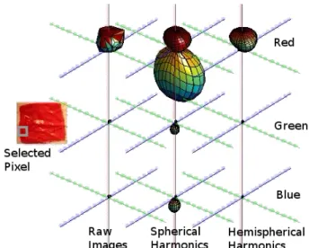
Figure 1: Capturing a BRDF slice and applying a reflectance model improves material classification. Sample captured image, 1 of 64 (left), Classification based on single image (middle), Classification based on Hemispherical Harmonic coefficients (right)
Abstract
Segmenting images into distinct material types is a very use-ful capability. Most work in image segmentation addresses the case where only a single image is available. Some meth-ods improve on this by collecting HDR or multispectral im-ages. However, it is also possible to use the reflectance properties of the materials to obtain better results. By ac-quiring many images of an object under different lighting conditions we have more samples of the surfaces Bidirec-tional Reflectance Distribution Function (BRDF). We show that this additional information enlarges the class of ma-terial types that can be well separated by segmentation, and that properly treating the information as samples of the BRDF further increases accuracy without requiring an ex-plicit estimation of the material BRDF.
1. Introduction
Material type classification of images is a fundamentl build-ing block of many important computer vision algorithms. It is also a useful tool in scientific applications ranging from environmental monitoring to art history. The simplest imag-ing source, which creates the hardest classification task, is a single grayscale image. Color and hyperspectral images provide more information, as do polarizing filters. We in-vestigate a different source of additional information: the angular variation of reflectance. While color and
polariza-tion all deal with a single point sample from the surface’s four dimensional BRDF, we capture a 2D slice of the BRDF, and show that this enlarges the class of material types that can be well separated. We also demonstrate how this infor-mation is best leveraged, comparing pixels by transforming the segmentation space using a BRDF model instead of raw measurements, achieving greater surface orientation invari-ance.
If an object is photographed twice from the same camera position, but with the light source in a different location, the resulting images may differ. This happens because the reflectance of many materials varies according to the in-coming and outgoing light directions. For example, shiny objects exhibit specular reflections, and diffuse objects ex-hibit the cosine term modulation. This variation is described by the material’s 4D Bidirectional Reflectance Distribution Function (BRDF), specifying the brightness observed in any outgoing direction (two dimensions) when light arrives from any incoming direction (two dimensions).
Capturing samples over the entire 4D BRDF can be imprac-tical for many applications, requiring images from many locations at many lighting conditions. Such a process re-quires solving for the stereo correspondences between all cameras, but this is difficult without dense sampling which requires either many cameras (which may be too expensive) or a moving camera (which may be too time-consuming). A single fixed camera and different lighting conditions cap-ture a 2D slice of the 4D BRDF. This relatively inexpensive process requires a modest amount of time and avoids the correspondence problem.
The BRDF slice provides two advantages over a single im-age. First, consider two pixels imaging different materials that appear similar under one lighting condition, but differ-ent under another. The BRDF slice aids in differdiffer-entiating these materials, despite their occasional similarity. Second, consider two objects made of the same material which ap-pear different due to their geometry (e.g. because one is angled to give a specular reflection, or the cosine term in-duces a brighter or dimmer reflectance). Here, the BRDF slice helps to identify these two objects as the same mate-rial by noting that their overall reflectance function has a similar shape.
Armed with a BRDF slice, material classification may be solved with a standard support vector machine (SVM) clas-sifier. Rather than directly compare the brightness values in each dimension, we can transform the observed bright-nesses to a new representation by fitting a parameterized partial BRDF model, covering just the 2D slice, and com-pare the resulting coefficients. We empirically evaluate this transformed representation against alternatives.
The principal contributions of this paper are,
1. A means to compare 2D BRDF slices acquired at pix-els that is invariant to surface orientation
2. Integration of this technique into the application of ma-terial type classification, with an empirical evaluation of this technique against alternate methods
This paper is organized as follows: section 2 relates this research to prior work, section 3 details our technique of BRDF slice comparison and its application to material clas-sification, and section 4 reports the results of an empirical evaluation against other methods. Section 5 discusses limi-tations of our technique, and section 6 concludes the paper.
2. Related Work
There has been a considerable amount of work in classi-fying materials with just a single image. This is a harder problem and, under unknown viewing and lighting condi-tions, becomes severely underconstrained for some materi-als. However, using statistical approaches to cluster similar materials has proved effective in handling such single im-age scenarios [14]. Another approach has been to exploit the reflectance properties of real world materials [4] . Additional information typically increases the number of materials that may be differentiated, for example using hy-perspectral imaging [7] or polarizing filters [15].
The entire BRDF may be captured by a goniometer or sim-ilar apparatus, as in [12] [3], but this process requires regis-tration between images. Without requiring regisregis-tration,
cap-turing thousands of lighting conditions from a single view allows good estimation of the BRDF of each material and classification into material types, which allows for applica-tions such as BRDF editing [10], [11]. In contrast, we use only dozens of lighting conditions rather than thousands. Hertzman et. al. develop an example-based approach to photometric stereo and material classification [8] [6]. They capture images under several lighting conditions of a scene with both a test object and a few reference objects of known geometry, and match the vector of brightnesses on the ob-ject to those on the test obob-ject. They use Euclidean dis-tance between raw brightness values and nearest-neighbor search, whereas we compare the parameters of a partial BRDF model directly.
Similarly, terrain-type classification from satellite imagery has been performed using images from several view direc-tions [1]. While these methods compare brightness values directly, we use an explicit BRDF model to compare pixels, without estimating a single BRDF for each material. Material classification and image segmentation are related but distinct applications, both depending on the compari-son of one pixel to another. Material classification typically treats each pixel independently, while image segmentation adds heuristics, such as enforcing that spatially contiguous areas are classified similarly unless separated by a strong edge detected in the images [13]. To explore the central question of pixelwise comparisons, we restrict our compar-ison to material classification rather than image segmenta-tion.
Many classifiers consider texture descriptors for the neigh-borhood surrounding a pixel, while we examine only a sin-gle pixel to isolate the pixel-comparison metric. Neighbor-hood descriptors may be extended to included BRDF mea-surements at each pixel. Alternatively, rather than consid-ering a neighborhood of pixels, each with a BRDF, a Bidi-rectional Texture Function may be used which incorporates spatial information [3] directly at each pixel.
3. Algorithm
3.1. Experimental Setup
To acquire BRDF slices, we constructed a hemispherical dome encircling the target object. A camera at the center of the dome records many images, each lit by a different lamp. This produces an image stack, where each pixel collects information for several lighting conditions for each color channel.
One case where the surface orientation can greatly affect the resulting reflectance is in paintings. In many cases the
surface orientation (from the thickness of paint or physi-cal properties of the medium) will effect the appearance of the painting, due to specular highlights and the cosine term. We used a similar principal in our test datasets, except we constructed our examples in ways such that the correct seg-mentation should be more apparent to the reader than with real paintings. We constructed our example datasets out of images of painted, crinkled paper. Each object contains sev-eral paints which differ either in their color, in their BRDF, or both.
Figure 2: An object was placed at the center of a dome that can provide lighting from many directions. A camera captures many images of the object, each under a different illumination.
3.2. Hemispherical Harmonics
Each pixel in the captured image stack is fit independently to a 2nd order Hemispherical Harmonic (HSH) representa-tion [5]. The HSH model uses shifted associated Legen-dre polynomials to bound the domain. This basis is better suited to pixel-comparison for material classification than the more general Spherical Harmonic (SH) model which is used so extensively in computer graphics. The SH model is defined over a complete spherical coordinate system; its coefficients are likewise estimated based on measurements over the whole sphere, and it may be used to interpolate new values over the whole sphere. The HSH model, on the other hand, is defined only over the upper hemisphere, and its coefficients are estimated based only on measurements there.
Since we restrict ourselves to opaque materials, input light-ing measurements are only made over the upper hemi-sphere. When fit with these measurements, the calculated SH coefficients interpolate unpredictably over the lower hemisphere, as seen in Figure 3. Though this poses no ficulty for relighting in graphics, it means that many dif-ferent sets of coefficients can produce similar interpolation across the upper hemisphere while giving different interpo-lation across the lower hemisphere. Thus, similar materials will not necessarily have similar SH coefficients. SH
coef-Figure 3: Actual measurements (left) are interpolated with Spherical Harmonics (SH) (middle) and Hemispher-ical Harmonics (HSH) (right). Since measurements are available over only the upper hemisphere, the SH model ex-trapolates randomly over the lower hemisphere. This leads to many possible sets of coefficients which all match the up-per hemisphere but have different coefficient values. The three rows show the BRDF slice fit separately to the red, green, and blue channels.
Figure 4: Attempting to perform classification of an object (left) by comparing Spherical Harmonic (SH) coefficients fails (middle), since the SH coefficients of similar materials may not be similar. Hemispherical Harmonic coefficients produce much more accurate classifications (right).
ficients for two pixels cannot then be directly compared; instead monte-carlo integration on the upper hemisphere would be required.
Since they are fit only by the set of measurements actually available, HSH coefficients are much more uniquely deter-mined by the material’s reflectance properties. Comparing the HSH coefficients of two pixels provides a good measure of BRDF similarity. As a result, performing classification with HSH coefficients leads to much more accurate classi-fication than with SH coefficients, as seen in Figure 4.
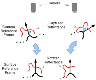
Figure 5: Measurements are rotated to the local surface reference frame. Before the measured BRDF slices of two pixels (left and right) can be effectively compared, the light directions must be rotated from the camera’s reference frame (top) to the local surface reference frame (bottom).
Figure 6: Using the BRDF slices without accounting for surface normal orientation leads to incorrect results (mid-dle). Rotating the light measurements to the surface refer-ence frame improves the consistency of the estimated coef-ficients, resulting in better classification (right)
3.3. Our Algorithm
The input to our algorithm is an image stack captured as described in section 3.1, and a set of labeled regions on the image defining a small patch of each material type. Pho-tometric stereo is applied to the image stack to estimate the normal direction at each pixel. The measured BRDF slice is used at each pixel independently to fit a second-order HSH model, with each color channel treated separately (9 coeffi-cients per color channel). For relighting purposes, the fitting would be done in the cameras reference frame. However, since we need to compare the coefficients directly, we want them to be invariant to the surface normal directions. The coefficients at each pixel should be expressed in that pixel’s local surface reference frame. This is achieved by rotat-ing all the incident lightrotat-ing samples before fittrotat-ing the HSH model, so that the surface normals are facing in the same
di-rection, as in Figure 5. Once this extra step is performed, we can fit the Hemispherical harmonic model to the data. Fail-ing to transform to the local surface reference frame leads to poor classifications, as in Figure 6.
We thus have two alternate representations of each pixel: either as a vector of brightnesses under different lighting directions, or as a vector of HSH coefficients. In both cases, the brightnesses or coefficients for each color channel are concatenated together into a single vector for each pixel. The set of vectors within each labeled region is used to train a multi-class Support Vector Machine (SVM) with a radial basis function kernel [2]. For each data set and each de-scriptor, the labeled pixels are split into a training and val-idation set to perform parameter selection via grid search, and the optimal parameters are used to train an SVM using the entire labeled region. This SVM is then used to classify each unlabeled pixel. Each pixel is classified separately.
3.4. Alternate Feature Vectors
We compared the algorithm using HSH coefficients as the feature vector to several simpler alternatives, which use the same SVM classifier but different data representations. The first is a single image from the image stack, giving a 3-element vector of the RGB color channels. A well-lit image was manually chosen in this case to improve the chances of correct segmentation. The second extracts the minimum, maximum, and median color for each pixel from the image stack, a 9-element vector. The maximum and minimum are calculated separately for each color channel, while the me-dian color is found as the 3-dimensional value minimizing the summed L1-distance to other images, over all lighting conditions in the image stack. The third alternative uses the vector of brightnesses from the entire image stack directly. This is a 192-element vector (3 color channels, 64 images).
3.5. Kernel Interpretation
Transforming each feature vector of brightnesses into a vec-tor of HSH coefficients redefines the pixel-comparison met-ric. This is equivalent to using the original vector of bright-nesses and applying a kernel within the SVM optimization. This “kernel trick” is often used to implicitly move a low-dimensional vector into a high low-dimensional space, so that point clouds which are not separable in the original space are separable in the kernel space.
We move to a lower dimensional space, but with the same goal. Our nonlinear transformation from brightness values to HSH coefficients creates a kernel space in which compar-isons are made, in which we hope the different materials’ point clouds are more easily separable.
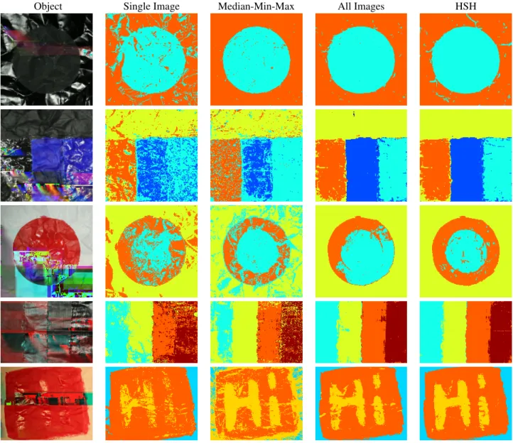
Object Single Image Median-Min-Max All Images HSH
Black Circle 12% 2% 2% 2%
Blue and Black Rectangles 23% 18% 4% 4%
Red Circles 20% 23% 14% 4%
Red and Black Stripes 20% 17% 2% 2%
Red Hi 10% 25% 4% 2%
Figure 7:Percentage of pixels classified incorrectly by each algorithm
Object Single Image Median-Min-Max All Images HSH
Figure 8:Comparisons of using single images, median-min-max, all images in the complete image stack, and HSH with our SVM classification.
4. Results
Five objects were imaged and classified as described in the previous section. Each object is made from white paper and several paints that vary in color and shininess, and is wrinkled to create a variety of surface orientations.
The classifications for each object, with each feature vec-tor, were compared to hand-labeled ground truth to iden-tify misclassified errors. Figure 7 reports the percentage of pixels wrongly classified. The HSH classifier consistently achieves higher accuracy than the alternative algorithms.
To better understand the types of classification errors made, consult Figure 8, showing classification errors visually. Classification with HSH coefficients is consistently the cleanest, and the single-image classification is consistently the noisiest.
Since specular reflections depend on the lighting direction and surface orientation, it is difficult for correct classifica-tions to be gleaned from a single image, as seen in the noise of the second column, “single-image”.
Two of the objects (the Blue and Black Rectangles and the Red and Black Stripes) are colored with four paints: two colors, in shiny and matte varieties. Notice that classifica-tion errors for these objects are nearly always show confu-sion between the shiny and matte verconfu-sions of the same color. This is expected; obviously-different colors are easy to dis-tinguish, but differences in specularity are more difficult to discern.
A few classification errors with the alternative feature vec-tors (though not with the HSH coefficients) are also made between one shiny color and the other shiny color, but never between one matte color and the other. Similarly, in the Red Circles, some classification errors are made between the shiny red paint and the white background. These er-rors indicate that the notion of “similarity” defined by these feature vectors includes both color and shininess. Whether this is desriable or not is application-dependent, but it is in-evitable when such materials are imaged.
Importantly, the HSH coefficients represent the data well with only a 27-element vector (9 coefficients for each of 3 channels), fit from the 192-element vector of the image stack. Also noteworthy is the fact that the simpler nonlin-ear transformation of the image stack into the Minimum, Maximum, and Median values captures a surprisingly large amount of information, giving significantly better classifi-cation than a single image.
5. Limitations
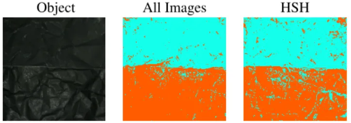
This paper focuses exclusively on single-pixel classifica-tion, and depends on separable training sets. Spots of matte paint were inadvertently sprayed onto the shiny part of the object in figure 9, and this texture was used in both train-ing and testtrain-ing data. The resulttrain-ing classification is not on par with the other objects. A classifier operating on neigh-borhoods of BRDF slices, or on BTF’s, might better handle textures such as this.
Object All Images HSH
Figure 9: An example where the our classification doesn’t work well due to textured material.
Complex 3D structures will exhibit self-shadowing, which we have not addressed. To perform classification in the presence of shadows, a robust estimation of the HSH co-efficients would be necessary.
The BRDF rotation step that we perform utilizes per-pixel surface normals. We compute these normals with photo-metric stereo, which assumes that materials follow a Lam-bertian reflectance model, and may therefore generate in-correct normals for non-diffuse materials. While it would be possible to generate more accurate normals using recent methods that do not require this diffuse reflectance assump-tion (such as the technique presented by Holroyd et al. [9]), we observe that our results were still improved significantly by the inclusion of the normal information.
Figure 10:Per-pixel normals (left) and albedo (center-left) computed with photometric stereo. Classification results us-ing only this data (center-right). The desired classification achieved using reflectance information (right).
We hypothesize that errors in photometric stereo are not random but result from confusion of the diffuse and spec-ular lobes, so that the half-angle between the view and lighting direction may be mistaken for the normal direction. When the light is at least as close to the normal as the view-point is, even an erroneous estimate is still an improvement
over assuming equal normals throughout the scene. In ad-dition, we note that reflectance information is essential, as different materials may have the same albedo. We show the result of performing the classification only on the recovered normal and albedo information in Figure 10.
Image segmentation builds on pixelwise material classifica-tion by adding heuristics to steer the resulting classificaclassifica-tion, for example by requiring spatially adjacent pixels to be clas-sified similarly unless a strong edge is found between them. The pixel-comparison technique developed here could be readily integrated into such an image segmentation algo-rithm.
6. Conclusions
Acquiring a BRDF slice rather than a single image al-lows superior material classification. We have presented a method to compare per-pixel 2D BRDF slice measure-ments using a BRDF model, without explicitly assigning a full 4D BRDF to the material. This comparison technique was integrated into a material classifier which was empiri-cally demonstrated to yield superior classification to alter-native pixel comparison methods.
References
[1] A. Abuelgasim, S. Gopal, J. Irons, and A. Strahler. Classi-fication of asas multiangle and multispectral measurements using artificial neural networks.Remote Sensing of Environ-ment, 57(2):79–87, August 1996.
[2] G. C. Cawley. MATLAB support vector machine toolbox (v0.50β) http://theoval.sys.uea.ac.uk/˜gcc/svm/toolbox. Uni-versity of East Anglia, School of Information Systems, Nor-wich, Norfolk, U.K. NR4 7TJ, 2000.
[3] K. Dana, B. Van-Ginneken, S. Nayar, and J. Koenderink. Re-flectance and Texture of Real World Surfaces. ACM Trans-actions on Graphics (TOG), 18(1):1–34, Jan 1999.
[4] R. O. Drora, E. H. Adelsonb, and C. Science. Estimating surface reflectance properties from images under unknown illumination.
[5] P. Gautron, J. Kˇriv´anek, S. N. Pattanaik, and K. Bouatouch. A novel hemispherical basis for accurate and efficient ren-dering. InRendering Techniques 2004, Eurographics Sym-posium on Rendering, pages 321–330, June 2004.
[6] D. B. Goldman, B. Curless, A. Hertzmann, and S. M. Seitz. Shape and spatially-varying brdfs from photometric stereo. InICCV ’05: Proceedings of the Tenth IEEE International Conference on Computer Vision (ICCV’05) Volume 1, pages 341–348, Washington, DC, USA, 2005. IEEE Computer So-ciety.
[7] J. Harsanyi and C. Chang. Hyperspectral image classifica-tion and dimensionality reducclassifica-tion: anorthogonal subspace projection approach.IEEE Transactions on Geoscience and Remote Sensing, 32:779–785, July 1994.
[8] A. Hertzmann and S. M. Seitz. Example-based photometric stereo: Shape reconstruction with general, varying BRDFs.
IEEE Transactions on Pattern Analysis and Machine Intelli-gence, 2005.
[9] M. Holroyd, J. Lawrence, G. Humphreys, and T. Zickler. A photometric approach for estimating normals and tangents.
ACM Transactions on Graphics (Proceedings of SIGGRAPH Asia 2008), 27(5):133, 2008.
[10] J. Lawrence, A. Ben-Artzi, C. DeCoro, W. Matusik, H. Pfis-ter, R. Ramamoorthi, and S. Rusinkiewicz. Inverse shade trees for non-parametric material representation and editing.
ACM Transactions on Graphics (Proc. SIGGRAPH), 25(3), July 2006.
[11] F. Pellacini and J. Lawrence. AppWand: Editing measured materials using appearance-driven optimization.ACM Trans. Graph., 26(3):54, 2007.
[12] S. Sandmeier, W. Sandmeier, K. Itten, M. Schaepman, and T. Kellenberger. The swiss field-goniometer system (figos).
Geoscience and Remote Sensing Symposium, 1995. IGARSS ’95. ’Quantitative Remote Sensing for Science and Applica-tions’, International, 3:2078–2080 vol.3, 10-14 1995. [13] J. Shi and J. Malik. Normalized cuts and image
segmenta-tion. IEEE Transactions on Pattern Analysis and Machine Intelligence, 22:888–905, 2000.
[14] M. Varma and A. Zisserman. A.: Statistical approaches to material classification. InIn: Proc. European Conf. on Com-puter Vision, 2002.
[15] L. B. Wolff. Polarization-based material classification from specular reflection. IEEE Trans. Pattern Anal. Mach. Intell., 12(11):1059–1071, 1990.