The water-soluble fraction of aviation jet fuels is examined using solid-phase extraction and solid-phase microextraction. Gas chromatographic profiles of solid-phase extracts and solid-phase microextracts of the water-soluble fraction of kerosene- and nonkerosene-based jet fuels reveal that each jet fuel possesses a unique profile. Pattern recognition analysis reveals fingerprint patterns within the data characteristic of fuel type. By using a novel genetic algorithm (GA) that emulates human pattern recognition through machine learning, it is possible to identify features characteristic of the chromatographic profile of each fuel class. The pattern recognition GA identifies a set of features that optimize the separation of the fuel classes in a plot of the two largest principal components of the data. Because principal components maximize variance, the bulk of the information encoded by the selected features is primarily about the differences between the fuel classes.
Introduction
Subsurface fuel spills and leaks represent the largest and most widespread cause of ground-water contamination in the United States. The Environmental Protection Agency has identified approximately 1.5 million underground storage tank sites in the continental U.S. in which fuels have spilled or leaked into the environment. Such spills and leaks on military property often involve aviation turbine fuels. Aviation fuels used by the Air Force, Army, and Navy include JP-4 (formally used by the Air Force and Army for flight operations within the continental U.S.), JP-5 (used by the Navy aboard ships), JPTS (used by the Air Force for special high-altitude flights), and JP-8 (which has replaced JP-4 as the standard turbine aviation fuel). The primary civilian aviation fuel used in the United States is Jet-A.
In a previously published study, Mayfield and Henley (1) char-acterized the water-soluble components of jet fuels using gas chromatography (GC). The water-soluble fraction consisted pri-marily of alkyl derivatives of benzene and naphthalene. These
analyses were performed by equilibrating pure water with the fuel, passing the aqueous phase through solid-phase extraction (SPE) cartridges loaded with C-18 modified silica, and then col-lecting the extracted organics with an organic solvent to yield a sample amenable to analysis by GC. The potential to identify the various jet-fuel classes by applying pattern recognition tech-niques to the GC profiles of the water-soluble fraction of non-kerosene-based jet fuels has been previously demonstrated (2).
In this study, pattern recognition techniques were used to type the gas chromatograms of the water-soluble fraction of kerosene-based jet fuels. The test data consisted of 133 gas chromatograms of solid-phase extracts of the water-soluble hydrocarbons col-lected from six different types of aviation turbine fuels (JP-4, Jet-A, JP-7, JPTS, JP-5, and AVGAS) and 108 gas chromatograms of solid-phase microextracts of the water-soluble hydrocarbons col-lected from four different types of kerosene-based jet fuels (Jet-A, JP-5, JP-8, and JPTS). This study, which is a logical extension of earlier efforts (3–7), was undertaken because of the difficulty in classifying the gas chromatograms of Jet-A, JP-5, JP-8, and JPTS fuels because of the similarity in their compositions.
Experimental
Neat samples of JP-4, Jet-A, JP-7, JPTS, JP-5, JP-8, and 100/130-octane aviation gasoline (AVGAS) were obtained from Wright Patterson Air Force Base (Dayton, OH) and Mukilteo Energy Management Laboratories (Mukilteo, WA). These fuel samples were splits from regular quality-control standards used by the two laboratories to verify the authenticity of the manufac-turer’s claims. The control standards constituted a representa-tive sampling of the fuels.
The water-soluble fraction was obtained by equilibrating 2 mL of a neat jet fuel with 250 mL of deionized water at ambient tem-perature while stirring gently for 12 h in a vessel designed by Burris and McIntyre (8) to maximize surface contact between fuel and water while avoiding mixing. Following equilibration, Abstract
Fuel Spill Identification Using Solid-Phase Extraction and
Solid-Phase Microextraction. I. Aviation Turbine Fuels
B.K. Lavine, D.M. Brzozowski, J. Ritter,andA.J. Moores Department of Chemistry, Clarkson University, Potsdam, NY 13699-5810 H.T. Mayfield
several milliliters of water was discharged from the vessel to ensure that the delivery tube was clear of fuel, and two 25-mL aliquots of the water phase were delivered into gas-tight syringes equipped with Luer-lock open shut valves. Thus, two 25-mL water samples could be prepared from a single fuel sample.
SPE and solid-phase microextraction (SPME) were used to characterize the 25-mL water samples containing the dissolved hydrocarbons. For the SPE procedure, each 25-mL aliquot was spiked with a solution of d10-ethylbenzene (98% atom purity, 1 µL/mL) (New England Nuclear, Boston, MA) in methanol (HPLC grade) (Fisher, Pittsburgh, PA) and then forced through a C-18 Sep-pak (Millipore Corporation, Bedford, MA) SPE car-tridge. The d10-ethylbenzene was used as an internal retention standard. Prior to use, each C-18 Sep-pak was pretreated using the procedure recommended by Millipore, which involved run-ning 2 mL of methanol through the cartridge followed by 5 mL of high-purity water.
After forcing the 25-mL water sample through the C-18 Sep-pak, the cartridge was partially dried with a 5-mL slug of air and extracted with 1 mL of carbon disulfide (glass distilled) (Aldrich, Milwaukee, WI). A 1-µL aliquot of each carbon disulfide extract was then injected onto a 60-m×0.25-mm fused-silica capillary column containing a 0.25-µm bonded polyethylene glycol sta-tionary phase (DBWAX, J&W Scientific, Folsom, CA), which was temperature programmed from 40°C to 200°C at 50°C per minute with an initial isothermal hold of 4 min. A splitless injection tech-nique was used with the injector port temperature set at 250°C. Gas chromatograms of the carbon disulfide extract were obtained
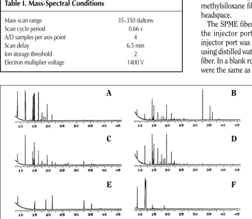
using a Hewlett Packard (Palo Alto, CA) 5987 GC–mass spectrom-eter (MS) with an HP-1000-F minicomputer running the RTE-6/VM operating system and RTE-RTE-6/VM GUMS Data System software. Hewlett-Packard-supplied software was used to subtract the mass 76 ion chromatogram from the total ion chromatogram of each sample in order to minimize the effect of carbon disulfide solvent on the sample chromatogram. The operating conditions of the MS are listed in Table I. Figure 1 shows GC profiles (i.e., total ion chromatograms) representative of the solid-phase extracts of JP-4, Jet-A, JP-5, and JPTS. The SPE data set, which consisted of 133 gas chromatograms, is described in Table II.
For the SPME procedure, each sample was placed in 40-mL VOA vials (Fisher Scientific) with one-hole screw caps and Teflon-faced septa (we did not add d10-ethylbenzene to the sam-ples in the SPME study because our experience with SPE demon-strated that its presence in the sample as a retention standard was unnecessary). Prior to the introduction of the sample, a microstirring bar was placed in a vial to permit the sample to be stirred by a magnetic stirrer during the SPME sampling period, which was 15 min. The stirring rate was reasonably high but not high enough to produce a vortex. In a previous study (9), we found that the actual rate of stirring was not a critical parameter. In retrospect, this result is not surprising because the purpose of stirring was to replenish the fiber-soluble components in the headspace, which were being depleted by adsorption into the SPME during sampling. We also had found that a 15-min sam-pling of the headspace was sufficient time to obtain a representa-tive sampling of the water-soluble compounds present in a jet fuel. In both the previous and current study, we used a 100µ poly-methylsiloxane fiber (SUPELCO, Bellefonte, PA) to sample the headspace.
The SPME fiber was preconditioned by first inserting it into the injector port of the GC for approximately 30 min. The injector port was set at 250°C. We then performed a blank run using distilled water as the sample to assess the cleanliness of the fiber. In a blank run the operating conditions for the GC and MS were the same as for an actual sample. If there were chromato-graphic peaks present, the preconditioning process was repeated until the blank run did not yield any chromatographic peaks.
GC profiles of the SPME microextracts were obtained using a Hewlett Packard 5890 GC equipped with a 5970B mass-selective detector, a split/splitless injection port, and a 30-m×0.25-mm fused-silica capillary column with 1-µm bonded and cross-linked 5% phenyl-substituted poly-methylsiloxane (DB-5, J&W Scientific). The GC oven was temperature pro-grammed from –10°C with an initial isothermal hold of 3 min to 250°C at a rate of 10°C/min followed by a 6-min final isothermal hold period. A splitless injec-tion technique was used with the injector port temperature set at 250°C. The purge delay time for the fiber was 1 min, and the fiber was left in the injection port for 10 min to ensure no carry over between runs. Table I. Mass-Spectral Conditions
Mass scan range 35–350 daltons Scan cycle period 0.66 s A/D samples per axis point 4
Scan delay 6.5 min
Ion storage threshold 2 Electron multiplier voltage 1400 V
Figure 1.GC profiles of water samples contaminated by jet fuels: (A) JP-4, (B) JP-5, (C) Jet-A, (D) JPTS, (E) JP-7, and (F) AVGAS. SPE was used to sample the dissolved hydrocarbons. For each gas chromatogram, they-axis corresponds with the total ion counts and thex-axis corresponds with time (min). Reprinted from reference 12 with the kind permission of Elsevier.
A B
C D
The injector port was fitted with a standard split/splitless liner. Subsequent studies have shown the advantage of using an SPME liner, but this product was not available at the time of this study. With regard to fiber aging, we did not observe any change in the GC profiles of the fuels over time that could be correlated with fiber aging. Fibers tended to be damaged by mishandling before reaching their lifetime.
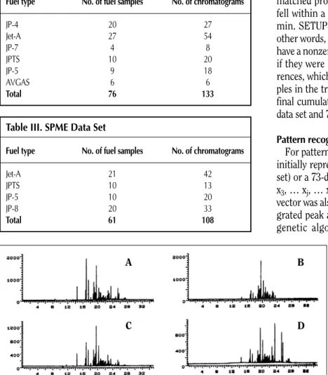
Operating conditions of the mass-selective detector were sim-ilar to those in the SPE study except that no scan delay was used, the ion storage threshold was 200, and the electron multiplier voltage was 2000 V. GC profiles representative of solid-phase microextracts of Jet-A, JPTS, JP-5, and JP-8 fuels are shown in Figure 2. The SPME data set consisting of 108 gas chro-matograms is summarized in Table III.
Data preprocessing
The gas chromatograms of the dissolved hydrocarbons were peak matched using a FORTRAN program called SETUP (10) that divided each gas chromatogram into intervals defined by so-called major peaks (i.e., peaks that were present in all of the chro-matograms). The major peaks were peak matched using
mass-spectral data acquired during the runs. Retention-time off-sets were then computed for the major peaks in each individual chromatogram. These offsets were the differences in retention time between the marker peaks in the reference chromatogram (which is selected by the user) and the chromatogram’s own marker peaks. The retention time offsets were 0.02 to 0.03 min. Finally, all of the peaks between the reference peak markers were adjusted by linear interpolation. This ensured that all GC peaks were expressed on the same time scale rotted on the majors (a major or marker peak was one that was easily recognizable in all gas chromatograms).
In order to standardize the retention time of the peaks eluting prior to the first major peak, it was necessary to use scaling fac-tors developed for the first pair of major peaks. Similarly, peaks eluting after the last major peak used a set of scaling factors developed for the final pair of major peaks. A template of unique peaks for the GC data was then constructed, with the peaks arranged according to their retention time. A preliminary data vector was generated for each GC profile by matching it against the template. If the peak was present, its area from the integra-tion report was assigned to the corresponding element of the vector. A peak not present was assigned a value of zero. For peak matching, specifying a tolerance window for acceptable reten-tion-time differences is generrally required. Thus, peaks were matched provided that differences in adjusted retention times fell within a specified tolerance window, which was set at 0.02 min. SETUP also computed the frequency of each feature. In other words, the number of times a particular peak was found to have a nonzero occurrence was computed. Features were deleted if they were below a user-specified number of nonzero occur-rences, which was set equal to 10% of the total number of sam-ples in the training set. The peak-matching procedure yielded a final cumulative reference file containing 48 peaks for the SPE data set and 73 peaks for the SPME data set.
Pattern recognition analysis
For pattern recognition analysis, each gas chromatogram was initially represented by a 48-dimensional data vector (SPE data set) or a 73-dimensional data vector (SPME data set, xj= (x1, x2, x3, … xj, … xp), where xjis the area of the jth peak). Each data vector was also normalized to constant sum using the total inte-grated peak area. The two GC data sets were analyzed using a genetic algorithm (GA) developed for pattern recognition (11–14) implemented in Matlab (Math Works, Inc., Natick, MA). The pattern recognition GA identified a set of features that optimized the sep-aration of the fuel classes in a plot of the two largest principal components of the data. Because principal components maximize variance, the bulk of the information encoded by these features is primarily about differences between the classes in the data set. Furthermore, the principal com-ponent plot functions as an embedded informa-tion filter. Sets of GC peaks were selected based on their principal component plots. A good principal component plot can only be generated using fea-tures whose variance or information is primarily about differences between the fuel classes. Thus, Figure 2.GC profiles of water samples contaminated by jet fuels: (A) Jet-A, (B) JPTS, (C) JP-8, and (D)
JP-5. SPME was used to sample the dissolved hydrocarbons. For each chromatogram, they-axis corre-sponds with the total ion counts and thex-axis corresponds with time (min).
A B
C D
Table II. SPE Data Set
Fuel type No. of fuel samples No. of chromatograms
JP-4 20 27 Jet-A 27 54 JP-7 4 8 JPTS 10 20 JP-5 9 18 AVGAS 6 6 Total 76 133
Table III. SPME Data Set
Fuel type No. of fuel samples No. of chromatograms
Jet-A 21 42
JPTS 10 13
JP-5 10 20
JP-8 20 33
principal component analysis (PCA) limits the search to these types of feature subsets, thereby significantly reducing the size of the search space.
A block diagram of the pattern recognition GA is shown in Figure 3. The pattern recognition GA differed from conventional GAs in several important respects. First, both adults and children were used to develop the new solutions. Potential solutions (i.e., feature subsets) were placed in two columns. In the first column, the solutions were ordered from best to worst on the basis of their fitness. In the second column, a copy of the same popula-tion (i.e., feature subsets) was randomly ordered with respect to fitness. The first row of the first column was then combined with the first row of the second column to yield new and potentially better solutions to the pattern recognition problem. Because the best feature subsets were always being used, each new genera-tion was expected to give better results than the previous gener-ation. However, each chromosome or potential solution had a chance of being selected (second column). This ensured that a significant degree of diversity was maintained during the search for a better solution. Typically, we set the selection pressure at 0.5 so that the top half of the ordered population was mated with strings or chromosomes from the top half of the so-called random population. Two new strings or potential solutions were generated for each pair of strings selected.
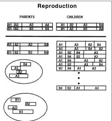
Second, the reproduction operator in the pattern recognition GA used a variation of three-point crossover to combine the binary strings to form new chromosomes. As in the case of simple three-point crossover, the length of each new string or solution was the same as the dimensionality of the data. However, the crossover operator used by the pattern recognition GA was not compelled to preserve order among exchanged string fragments. This safeguarded the loss of information or features in the population (see Figure 4). This variation of three-point crossover was also useful in searching for good string arrange-ments. When it is supposed that the current population has bad ordering, in which features with a high synergism are spaced at great distances, simple crossover would probably destroy these important allele packets. However, there would be a chance to obtain good ordering if a crossover operator was used with a reordering algorithm embedded in it.
Third, the fitness function of the pattern recognition GA emu-lated human pattern recognition via machine learning to score the feature subsets. In order to track and score the principal com-ponent plots, class and sample weights (which are an integral part of the fitness function) were computed (see equations 1 and 2). Class weights added up to 100, whereas the sample weights in a
class added up to a value equal to the corresponding class weight. CW(c) CW(c) = 100 ———— Eq. 1 ∑CW(c) c SW(s) SW(s) = CW(c) ———— Eq. 2 ∑SWc(s) s∈c
Each principal component plot that was generated for each feature subset after it was extracted from its chromosome was scored using the K-nearest neighbor (K-NN) classification algo-rithm (15). For a given data point in the principal component plot, Euclidean distances were computed between it and every other point. These distances were arranged from smallest to largest. A poll was then taken of the point’s K-NNs. For the most rigorous classification, k equaled the number of samples in the class to which the point belonged. The number of nearest neigh-bors with the same class label as the sample point in question, the so-called sample hit count (SHC), was computed (0≤SHC(s)
≤Kc). Scoring the principal component plot (see equation 3) became a simple matter.
1
F(d) =∑∑——×SHC(s)×SW(s) Eq. 3
c s∈c KC
In order to understand the scoring of a principal component plot, a data set with two classes should be hypothetically consid-ered (class 1 has 10 samples and class 2 has 20 samples). At gen-eration 0, each class is assigned equal weights, and the samples in a given class has the same weight. Thus, each sample in class 1 has a sample weight of 5, whereas each sample in class 2 has a weight of 2.5. It is supposed that a sample from class 1 has as its nearest neighbors seven class 1 samples in a principal compo-nent plot developed from a particular feature subset. With this in mind, SHC/K = 0.7 and (SHC/K)*SW = 0.7*5, which equals 3.5. By summing (SHC/Kc)*SW for each sample, each principal
com-ponent plot can be scored.
Fourth, the fitness function of the GA was able to focus on samples or classes (or both) that were difficult to classify by changing or boosting their weights over successive generations. In order for boosting, the sample hit rate (SHR) was computed. The SHR was the mean value of SHC/Kcover all feature subsets
produced in a particular generation: 1 ø SHCi(s)
SHR(s) = —∑———— Eq. 4
ø i=1 K
Boosting was then performed in three stages. First, the class hit rate (CHR) was computed. CHR was the average SHR for all samples in a class.
CHRg(c) =AVG(SHRg(s):∀s∈c) Eq. 5
Classes with a low CHR were weighted more heavily than classes whose samples scored well. Second, class and sample weights were adjusted using a perceptron. The user must set the momentum, P.
CWg+1(s) = CWg(s) + P(1 – CHRg(s)) Eq. 6 SWg+1(s) = SWg(s) + P(1 – SHRg(s)) Eq. 7 Third, after a certain number of generations, the class weights will not change. Equation 6 was turned off and the GA focused exclusively on the troublesome samples via equation 7.
During each generation, class and sample weights were updated using the class and SHRs from the previous generation (g + 1 was the current generation, whereas g was the previous generation). The aforementioned procedure, which involved evaluation, reproduction, and adjustment of internal parameters
(i.e., boosting of the potential solutions), was repeated until a specified number of generations were executed or a feasible solu-tion was found.
The advantages of using the pattern recognition GA for feature selection were three-fold. First, chance classification would not be a problem because the bulk of the variance or information content of the feature subset selected was primarily about the class membership problem of interest. Second, features that contain discriminatory information about a particular classifica-tion problem would be expected to be correlated, which was why feature selection methods based on PCA were ideally suited for carrying out feature selection. Third, the PCA routine of the fit-ness function was able to dramatically reduce the size of the search space because it could correctly assess the true dimen-sionality of the data, ensuring that only those regions of the solu-tion space with informasolu-tion about the problem of interest were investigated.
Results and Discussion
The first step in the study was to apply PCA to the data (16). PCA is a method for transforming the original measurement variables into new, uncorrelated variables called principal com-ponents. Each principal component was a linear combination of the original measurement variables. Using this procedure was analogous to finding a new coordinate system that is better at conveying information present in the data than axes defined by the original measurement variables. The new coordinate system was linked to variation in the data. Often, only two or three prin-cipal components were necessary to explain all of the informa-tion present in a data set that had a large number of interrelated measurement variables. Thus, PCA could be applied to high-dimensional data in order to affect high-dimensionality reduction, identify and display structure, classify samples, or identify out-liers.
Figure 5 shows a principal component map developed from the 48 GC peaks obtained from the 133 SPE gas chromatograms. The map of the two largest principal components of the data accounted for 65% of the total cumulative vari-ance. Each gas chromatogram was represented by a point in the principal component map. JP-4, AVGAS, and JP-7 were well-separated from one another and from the gas chromatograms of Jet-A, JP-5, and JPTS in the principal component plot, suggesting that information characteristic of fuel type was present in the gas chro-matograms of the water solubles. The overlap of JP-5, Jet-A, and JPTS fuel samples in the principal component map suggested that gas chro-matograms of these fuel materials shared a common set of attributes, which is not surprising because of the similarity in their physical and chemical properties (e.g., flash point, freezing point, vapor pressure, and distillation curve) (17). Mayfield and Henley (1) observed that gas chro-Figure 4.Crossover operator employed in the pattern recognition GA
(reference 11).
Figure 5.A plot of the two largest principal components developed from the 48 GC peaks of the 133 SPE gas chromatograms. Each gas chromatogram is represented by a point in the principal compo-nent map: (1) JP-4, (2) Jet-A, (3) JP-7, (4) JPTS, (5) JP-5, and (6) JP-8. Reprinted from reference 12 with the kind permission of Elsevier.
matograms of kerosene-based fuels (e.g., Jet-A, JP-5, and JPTS) were more difficult to classify than gas chromatograms of other types of processed fuels because of the similarity in the overall hydrocarbon composition of these fuel materials. Nevertheless, Mayfield and Henley were able to find fingerprint patterns within the gas chromatograms of kerosene-based fuels characteristic of fuel type, which motivated us to investigate the existence of these types of patterns in the SPE data set.
A GA for pattern recognition was used in the study to uncover features characteristic of the chromatographic profile of each fuel class. The GA identified features by sampling key feature subsets, scoring their principal component plots, and tracking those samples or classes that were most difficult to classify. The boosting routine used this information to steer the population to an optimal solution. After 100 generations, the GA identified two
standardized retention time windows (features 9 and 23) whose plot showed clustering of the fuel samples according to fuel type (see Figure 6). This suggested that information about fuel type was contained within the gas chromatograms of the water-sol-uble components. The ease of classifying these highly complex mixtures by selective fractionation becomes apparent when taking into account the fact that an equilibration time of only 3 h is necessary to obtain a reproducible profile of the water-sol-uble components of a jet fuel (18).
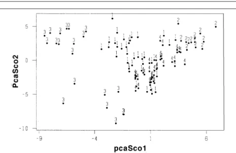
Figure 7 shows a plot of the scores of the two largest principal components of the 73 GC peaks obtained from the 108 SPME gas chromatograms. The map of the two largest principal compo-nents of the data accounted for 60% of the total cumulative vari-ance. Each gas chromatogram was represented by a point in the principal component map. JPTS and JP-5 were well-separated from each other and from the gas chro-matograms of Jet-A and JP-8 in the principal component map, whereas the gas chro-matograms of the Jet-A and JP-8 fuel samples overlapped. The fact that SPME did a better job at discriminating between Jet-A and JP-5 than SPE can be attributed to the fact that headspace SPME is better than SPE at extracting the water-soluble components of the fuels (9). SPME was also more convenient than SPE for sampling organics from aqueous solutions and was the method of choice for those situations in which the analysis was lim-ited to the headspace of the sample.
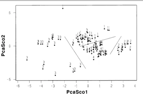
Using the pattern recognition GA, feature selec-tion was performed to identify peaks that could differentiate the gas chromatograms of JP-8 fuels from Jet-A fuels. This particular pattern recogni-tion problem was deemed important because of the change from JP-4 to JP-8 as the principal U.S. Air Force fuel. Figure 8 shows a score plot of the two largest principal components developed from 13 GC peaks identified by the GA. The 13 peaks spanned the entire gas chromatogram and, iden-tified by the pattern recognition GA, allowed the fuels to cluster by type in a plot of the two largest principal components of the data.
In order to test the predictive ability of the 13 GC peaks identified by the pattern recognition GA, we would need an external prediction set con-sisting of gas chromatograms of the microex-tracts of the water-soluble components of the weathered jet fuels. Unfortunately, GC profiles of the water-soluble components of weathered jet fuels were not obtained when this study was per-formed. Because the two largest principal compo-nents captured the bulk of the variance of the feature subset in question, it was unlikely that chance classifications could explain the clus-tering of the fuel samples by type in a map of the two largest principal components of the 13 GC peaks. Monte Carlo simulation studies performed in our laboratory to address this issue indicated that the likelihood of obtaining such a principal Figure 6.A plot of standardized retention time window 9 versus standardized retention time window
24 for the 133 SPE gas chromatograms. Each gas chromatogram is represented by a point in the prin-cipal component map: (1) JP-4, (2) Jet-A, (3) JP-7, (4) JPTS, (5) JP-5, and (6) JP-8. The clustering of the fuel samples according to fuel type in the feature map is evident. Reprinted from reference 12 with the kind permission of Elsevier.
Figure 7.A plot of the two largest principal components developed from the 73 GC peaks of the 108 SPME gas chromatograms. Each gas chromatogram is represented by a point in the principal compo-nent map: (1) Jet-A, (2) JPTS, (3) JP-5, and (4) JP-8. Reprinted from reference 12 with the kind permis-sion of Elsevier.
component plot (as shown in Figure 8) resulting from chance is essentially zero. Because the neat jet fuel samples chosen for this study constituted a representative sampling of these fuels, we believe that legitimate chemical differences in the water-soluble components of the fuels characteristic of type exist that can be exploited by the methodology discussed in this study.
Conclusion
The clustering of the fuel samples according to fuel type in the principal component plots generated from the SPE and SPME data sets (see Figures 6 and 8) suggests that fuel-spill identifica-tion rotted on the water-soluble components of jet fuels is fea-sible for both kerosene and nonkerosene-based jet fuels. Thus, it is logical to consider the direct implementation of the selective fractionation scheme described in this study as an integral com-ponent of the methodology used by the United States Air Force to identify fuels recovered from subsurface environments.
Acknowledgments
Dr. Lavine would like to acknowledge the financial support of the Air Force Office of Scientific Research (Bollings Air Force Base, Washington, D.C.) through their Summer Faculty Research Program. Dr. Ritter would like to acknowledge the financial support of the Air Force Office of Scientific Research through their Summer Graduate Student Research Program. D. Brzozowski would like to acknowledge the financial support from Clarkson University’s Honors Program.
References
1. H.T. Mayfield and M. Henley.In Monitoring Water in the 1990’s: Meeting New Challenges. J.R. Hall and G.D. Glayson, Eds. ASTM, Philadelphia, PA, 1991, pp. 578–97.
2. B.K. Lavine. Environmental applications of pattern recognition tech-niques.Chemolab15:219–30 (1992).
3. B.K. Lavine, X. Qin, A. Stine, and H.T. Mayfield. Application of pat-tern recognition techniques to problems in advanced pollution monitoring.Process & Quality Control2:347–55 (1992). 4. B.K. Lavine, H.T. Mayfield, P.R. Kroman, and A. Faruque. Source
identification of underground fuel spills by pattern recognition anal-ysis of high-speed gas chromatograms.Anal. Chem.67:3846–52 (1995).
5. B.K. Lavine, A. Stine, and H.T. Mayfield. Gas chromatography—pat-tern recognition techniques in pollution monitoring.Anal. Chim. Acta.277:357–67 (1993).
6. B.K. Lavine, A.B. Stine, H. Mayfield, and R. Gunderson. Application of high-resolution computer graphics to pattern recognition anal-ysis.J. Chem. Inf. Comput. Sci.33:826–34 (1993).
7. B.K. Lavine, R.K. Vander Meer, L. Morel, R.W. Gunderson, J.R. Han, and A. Stine. False color data imaging: a new pattern recognition technique for analyzing chromatographic profile data. Microchemical J.41:288–95 (1990).
8. W.G. MacIntyre and D.R. Burris. A novel extraction vessel for char-acterizing water soluble components of processed fuels.Environ. Toxicol. Chem.4:371–80 (1985).
9. J. Ritter, V.K. Stromquist, H.T. Mayfield, M.V. Henley, and B.K. Lavine. Solid phase micro-extraction for monitoring jet fuel compo-nents in groundwater.Microchemical J.54:59–71 (1996). 10. H.T. Mayfield and W. Bertsch. SetUp: a chromatogram transducing
program.J. Comput. Appl. Lab.1:130–36 (1983).
11. B.K. Lavine, A. Moores, and L.K. Helfend. A genetic algorithm for pattern recognition analysis of pyrolysis gas chromatographic data. J. Anal. Appl. Pyrolysis50:47–62 (1999).
12. B.K. Lavine, D. Brzozowski, A.J. Moores, C.E. Davidson, and H.T. Mayfield.Anal. Chim. Acta437:233–46 (2001).
13. B.K. Lavine, A.J. Moores, H.T. Mayfield, and A. Faruque. Genetic algorithms applied to pattern recognition analysis of high speed gas chromatograms of aviation tur-bine fuels using an integrated Jet-A/JP-8 data base. Microchemical J.61:69–78 (1999).
14. B.K. Lavine, J. Ritter, A.J. Moores, M. Wilson, A. Faruque, and H.T. Mayfield. Source identifica-tion of underground fuel spills by solid phase micro-extraction/high-resolution gas chromatog-raphy/genetic algorithms. Anal. Chem.72(2): 423–31 (2000).
15. K. Fukunaga.Introduction to Statistical Pattern Recognition, 2nd ed. Academic Press, New York, NY, 1990.
16. I.T. Jolliffe. Principal Component Analysis. Springer-Verlag, New York, NY, 1986.
17. Handbook of Aviation Fuel Properties. Coordinating Research Council Inc., Atlanta, GA, 1983.
18. B.K. Lavine.Solid Phase Micro-Extraction Applied to the Problem of Fuel Spill Identification. Summer Faculty Research Program, Air Force Office of Scientific Research, Bollings Air Force Base, Washington, D.C., August 1995.
Manuscript accepted May 14, 2001. Figure 8.A plot of the two largest principal components developed from the 13 GC peaks identified
by the pattern recognition. Each gas chromatogram is represented by a point in the principal compo-nent map: (1) Jet-A, (2) JPTS, (3) JP-5, and (4) JP-8. The clustering of the samples according to fuel type in the principal component map is evident.