66
Comparative Analysis of Public Debt Management and Economic
Growth in Nigeria
Ajayi, Samuel Abiodun1
Landmark University Omu Aran, Nigeria. ajayi.abiodun@lmu.edu.ng Okunlola, Oluyemi Adewole
University of Medical Sciences, Ondo State, Nigeria. ookunlola@unimed.edu.ng
Tony Ikechukwu Nnwanji Landmark University Omu Aran, Nigeria
Nnwanji.tony@lmu.edu.ng Otekunrin Adegbola Olubukola Landmark University Omu Aran, Nigeria.
otekunrin.adegbola@lmu.edu.ng Oladipo Olufemi Adebayo Landmark University Omu Aran, Nigeria.
oladipo.olufemi@lmu.edu.ng Awonusi, Frank Dayo
Landmark University Omu Aran, Nigeria. awonusi.frank@lmu.edu.ng
Abstract
The study examined the impact of public debt management on the economic growth of Nigeria putting into consideration the influence of military and civilian rule for the period of 1983-2015. The estimation techniques employed in the study is Error Correction Model. To avoid spurious regression due to the problem of non-stationarity of data, the Augmented Dickey Fuller test was used to check for the presence of a unit root, Ljung-Box Q-statistics test for autocorrelation and Breusch-Pagan Godfrey test for Heteroscedasticity in the variables. The results showed a significant long run relationship exists between public debt management and economic growth in Nigeria under the military, but a relative low impact on economic growth of Nigeria under the civilian rule. This may due to poor management strategies and indiscriminate borrowing by states of the federation without check and caution by the civilian regime. It was advised that public borrowing should be channelled to developmental projects and productive sectors of the economy that will stimulate growth in the long run.
Keywords: Public Debt; Public Debt Management; Debt overhang; Economic growth JEL CLASSIFICATION: H63
67 Introduction
Not all countries can boast of being self-dependent at every point in time, so they need to borrow in order to take care of the needs of their citizen. Udeh, Ugwu and Onwuka (2018) are of the view that this often results to debts. Countries indulge in debt to boost economic growth and reduce poverty (Tajudeen, 2012). Ijeoma (2013) and Tajudeen (2012) are of the view that in order to encourage growth, countries at early stages of development such as Nigeria borrow to argument what they have because of dominance of small stocks of capital. Nigeria borrowed from external sources mainly for investment purposes, which is macro-economic aid for financing transitory balance of payment deficit and avoid budget constraint so as to boost economic growth and reduce poverty (Anochie & Ude, 2015).
Public debt becomes an issue when it is difficult to pay back and this is a major problem faced by most developing countries in the world as they tend to use a high percentage of their GDP to service such debts each year. Over the years, a sizeable chunk of the nation‟s hard earned revenue (foreign earning) has been expended on debt servicing which has caused some setbacks in the nation‟s economy (Ajayi & Oke, 2012).
One major obstacle for Nigeria‟s economic development over the last two decades has been its crippling debt overhang (Yusuf, Idowu, Okunnu, & Adeyemi, 2010). Poorly structured debt in terms of maturity, currency, or interest rate composition, and large and unfunded contingent liabilities have been important factors in inducing or propagating economic crises in many countries throughout history (International Monetary Fund & World Bank, 2001). The quest for economic growth and development forced Nigeria to acquire external debt (Udeh et al, 2018). Public debt management is the process of
establishing and executing a strategy for managing government‟s debt in order to raise the required amount of funding at the lowest possible cost over medium to long run, which is consistent with a prudent degree of risk (International Monetary Fund & World Bank. 2014). Debt management is commonly considered as a programme or policy that helps debtors in acquiring and clearing off debts (Arit, 2013). One of the major problems faced by Nigeria is its inability to manage its debt effectively. This brought about the establishment of the Debt Management Office in 2000 which is charged with the management of the country‟s public debt. So far, the Debt Management Office has been unable to manage Nigeria‟s increasing debt profile. Over the past decade, a broad consensus has developed that good public debt management can help countries reduce their borrowing cost, contain financial risk, and develop their domestic debt market (Tomás & Sundararajan, 2008). Arit (2013) is of the view that countries with good management policies will have a better chance at developing institutions with high quality in terms of achieving its functions. This study seeks to analyse the public debt profile of Nigeria and the measures put in place to manage its debt and how it affects the economy as a whole.
“The rising domestic debt emanated from the challenging fiscal position resulting from dwindling oil revenue coupled with the need to implement several reform initiatives at both national and sub-national levels of government” (Barbara, Eric, & Colleen, 2015: 8). Increase in domestic debt has the tendency to increase interest rates which results in the crowding out of the private sector from the local credit market which in the long run have a negative effect on the economy. Debt overhang phenomenon is where substantial resources are used for debt servicing such that it stifles economic
68 growth (Udeh et al, 2018). „The servicing of debt absorbs budgetary and foreign exchange resources, and the absence of any benefits accruing from the investment of the original loan will have a net negative effect on a government‟s ability to fund its social expenditure programmes‟ (United Nations, 1999). The major cause of the increase in the debt burden of Nigeria is its inability to manage its debts, both internal and external. Good public debt management can help countries like Nigeria to reduce their borrowing cost, contain financial risk, and develop their domestic debt market (Tomás & Sundararajan, 2008). What has compounded the debt problem of Nigeria mostly can be said to be the unstable governance both in the federal and state levels. The shift between the military and civilian regimes has brought a lot of distortion in the development plan thereby hindering economic growth.
The motives of borrowing between the two regimes (Military and Civilian) had also impacted on the management and repayment process. While the military will borrow for essential development projects, the civilian government might borrow to finance projects that is not of economic value to the citizens but to score a political point. Debt profile also increases during civil rule since they usually have easy access to funds in the Capital Market and foreign aids due to the support they have from internationals fronts. Another applauding thing is that the management of funds are sometimes misappropriated through embezzlement and diversion funds for own private use.
The main aim of this study is to ascertain the effect of public debt management on the Nigerian economy by giving a comparative analysis of the influence of military and civilian rules on the increasing debt burden of the country covering a period of 32 years (1983-2015). This period is divided into two periods;
1983-1999, signifying the military regime and 1999-2015, signifying the civilian rule in order to give an in-depth analyses of Nigeria‟s public debt.
Section one contains the general introduction and section two is the review of literature. Section three provides the methodology employed in the study while section four presents results from the analysis and discussion of findings. Section five concludes the study with relevant policy implications and recommendations. Literature Review
The aim of public debt is to boost economic growth and development. But when the debt burden of a country is on the high side, debt servicing becomes difficult which tends to be a serious threat to economic growth and development of any country. Different researchers have therefore sought to investigate the implication of public debt burden on the economies of debtor nations and have come up with different views.
Ijeoma (2013) carried out a study on an empirical analysis of the impact of debt on the Nigerian economy. Variables of external debt stock, external debt service payment and exchange rate were used to determine their effect on Gross Domestic Product (GDP), and Gross Fixed Capital Formation (GFCF) for the period 1980-2010. Secondary data were used for the study which were analysed with linear regression. The result of the study was that Nigeria‟s external debt stock has a significant effect on her economic growth and there is also a significant relationship between Nigeria‟s debt service payment and her Gross Fixed Capital Formation.
Onuorah, Chi-Chi and Ogbonna (2013) examined deficit financing and the growth of Nigeria economy. The study made use of data from publications of the Central Bank of Nigeria Statistical bulletin between 1981 and 2012. The researcher
69 made use of descriptive statistics, Ordinary Least Square (OLS), Diagnostic test, ADF unit root, Johansen Co-integration and pairwise Granger causality test. The result showed that deficit financing is statistically significant and positively related to economic growth in Nigeria. This suggests that both domestic debt and external debt liability contributes effectively to the settlement of Nigeria debt. The result from the regression analyses shows that domestic debt and external debt remains the crucial source of financing Nigeria debt. A conclusion was drawn that a long-run equilibrium relationship exists between the dependent and independent variables, and it was assumed that the deficit financing assert sufficient influence on growth in the debt management and services in Nigeria. The researcher suggests an appropriate combination of internal and external debt ratio with a close monitoring situation. They also recommended that the Policy makers should control the level of deficits to ensure that it is within this level and a decrease is also required in the level of the deficits; this could strengthen the exchange rate and as well control inflationary pressure in Nigeria. Dereje and Joakim (2013) studied the effect of external debt on economic growth. They examined whether external debt affects the economic growth of selected heavily indebted poor African countries through the debt overhang and debt crowding out effect. This was carried out by using data for eight heavily indebted poor African countries between 1991 and 2010. The result from estimation shows that external debt affects economic growth by the debt crowding out effect rather than debt overhang. Furthermore, in an attempt to mark out debt servicing history, the thesis found that the selected countries are not paying (servicing) more than 95% of their accumulated debt.
Madu et al (2015) examined the political economy of external debt
management in Nigeria with a special focus on strategies, issues and challenges. They adopted a descriptive research method and content analysis approach whereby data were mainly obtained through extensive literature from books, scholarly articles and internet sources. Some abnormalities were discovered in the external debt which tends to have a negative effect on the Nigerian political economy. The abnormalities listed include; “unfavourable loan term; epitomized by compounding of interests, poor management of credit facilities, fragile economic base, overdependence on foreign aids as well as paucity of statistics on loans” (p.23). They are of the view that this led to underperformance of almost all the key economic indices of the Nigerian state thereby creating poor infrastructural development and a very weak manufacturing sector. A conclusion was made that unless deliberate attempt is made to turn the designed strategies already put in place into meaning results, the country‟s debt stock will continue to skyrocket which in turn accumulates into a huge debt burden on its developmental, socio-political and economic strides. As a result of these, a recommendation was made that the “Nigerian state must manage its credits better by allocating the funds to the real sectors of the economic base, and deliberate policy must also be embarked upon to encourage the development of virile productive sector for sustainable economic development” (p.23).
Adesola et al (2015) studied the Nigeria debt portfolio and its implications on economic growth. They examined the relationship between economic growth and debt variables for the period 1981-2012 using Vector Error Correction Model (VECM) approach. They are of the view that “Debt-to-GDP ratios of 21.4% (domestic debt) and 26.9% (external debt) revealed that Nigeria can benefit from borrowed funds provided it stays below
70 these limits and the repayment conditions are favourable. Hence, funds channelled towards developmental efforts will have positive ripple effects on the economy” (p.87).
Udeh; Ugwu & Onwuka (2018) researched the Nigeria experience on external debt and economic growth. Ex-post facto research design was used in the study and secondary source of data collection were used to get information on the variables of Gross Domestic Product (GDP) and External Debt Service Payment. The researchers concluded that exchange rate fluctuation had positive impact on the Nigerian economy while external debt stock and debt service payment had negative impact on the same economy. The recommendation made was that “the Debt Management should set mechanism in motion to ensure that loans were utilized for purposes for which they were acquired as well as set a ceiling for borrowing for states and federal governments based on well-defined criteria”(p.33).
In conclusion, the above empirical studies identified the fact that most researchers focused on the impact of external debt on the economic growth of Nigeria while few focused on the impact of domestic debt which covers a high percentage of the public debt burden of the country which in turn affects economic growth. This study, therefore, focuses on how public debt (external debt and domestic debt) and its management affect the economic growth of Nigeria and goes further to examine the influence military and civilian rules have on the increasing debt burden.
Methodology
The methodology adopted in this study is the independent t-test and Error Correction Model. The independent t-test is used to check for means difference between the two regimes while error correction
model is used to determine the short run dynamics and the speed of adjustment. As a custom in times series analysis related problem, Augmented Dickey Fuller (ADF) and Phillip Perron are used to determine level of integration of the variables, Johansen co-integration is employed to investigate long run economic relations among the variables. Prior to the estimation of Error Correction Model, optimum lag lengths are determined using several criteria.
Model Specification
The main aim of this study is to examine the effect of public debt management on economic growth in Nigeria, taking into consideration the influence of civilian and military rule. The model is adopted from Abula and Mordecai (2016). The model is specified of the functional form:
RGDP= (DDS, EDS, ESP, CAP, LAB) --- Equation 1 Where:
RGDP = Real Gross Domestic Product DDS = Domestic Debt Stock
EDS = External Debt Stock
ESP = External Debt Service Payment CAP = Domestic Capital Formation LAB = Labour
The model is specified of its stochastic form: RGDP = β0 + β1DDS + β2EDS + β3ESP+ β4CAP + β5LABμ Where: μ = Error term β0 = Intercept Explicit form:
The error correction model specification at maximum lag length of two is of the form:
Military Model
( ) ( ) ( ) ( ) ( ) ( )
71 ( ( )) ( ( )) ( ( )) ( ( )) ( ( )) ( ( )) ( ) ………Equation 2 Civilian Model ( ) ( ) ( ) ( ) ( ) ( ) ( ( )) ( ( )) ( ( )) ( ( )) ( ( )) ( ( )) ( )………Equation 3 Pooled model ( ) ( ) ( ) ( ) ( ) ( ) ( ( )) ( ( )) ( ( )) ( ( )) ( ( )) ( ( )) ( ( )) ( ( )) ( ( )) ( ( )) ( ( )) ( ( )) ( )
Where is difference operator, is the intercept, to are the parameter while ect(-1) is lag value of OLS residual. In the equation above, if 2 is positive and significant, it denotes a positive impact on the dependent variable.
Real Gross Domestic Product (GDP) is the monetary value of all finished goods and services produced within a country‟s borders in a specific time period (Investopedia, 2016). It is used to capture economic growth in this study because it is adjusted for inflation which therefore provides a more accurate figure.
Data Analysis and Discussion of Results Test of difference of mean
The t-test of mean difference result for the regimes is presented in Table 1 for all the variables considered in the study. The test indicates that the mean level of the majority of the variables are significantly higher in the civilian regime as against the military with the exception of capital and labour
Table 1: Test of difference of mean between the two regimes
Regime N Mean Std. Deviation Std. Error
Mean t-statistic (p-value) rgdp Military 16 18138.6219 2883.69492 720.92373 -6.649 (0.000) Civilian 17 44400.1794 15535.82634 3767.9913 5 dds Military 16 203.4444 201.74795 50.43699 -4.666 (0.000) Civilian 17 3420.3171 2748.14735 666.52363 eds Military 16 348.4806 272.16912 68.04228 -4.482 (0.000) Civilian 17 2034.2265 1479.86405 358.91975 dsp Military 16 6.0650 13.48121 3.37030 -5.034 (0.000) Civilian 17 382.2880 298.39965 72.37254 esp Military 16 22.7625 17.29324 4.32331 -2.656 (0.000) Civilian 17 290.6000 402.59928 97.64467 Cap Military 16 38502.8950 9513.73688 2378.43422 0.357 (0.723) Civilian 17 35769.0624 29146.00160 7068.94372 Lab Military 16 24424.4656 12263.75771 3065.93943 0.545 (0.590) Civilian 17 21865.1082 14552.61493 3529.52756
Source: Author‟s compilation (2018). Note: P-value less than 0.05 indicates significant difference at 5% confidence level
72 The mean results in Table 1 shows that DDS, EDS, DSP and ESP have higher values in the civilian regime than the military regime. This is unlike the CAP and LAB where there are light differences between the two with the military having a higher capital formation of 38502.8950 and civilian 35769.0624, and that of labour is also higher with military having 24424.4656 and civilian, 21865.1082. The total debt structure is lower in military regime and higher in the civilian regime during the period under investigation.
Unit Root Test
The unit root test was performed to check for the presence of unit root in a time series. This test is carried out using the Augmented Dickey Fuller (ADF) test and the Phillips-Perron (PP) test in order to correct for autocorrelation and heteroscedasticity in the errors. The ADF and PP test are carried out using Eviews 9 software package and the results from the test are presented in Table 2.
Table 2: ADF Test for Stationarity
VARIABLE ADF at LEVELS ADF at 1ST Difference Order of Integration LRGDP 0.552197 -3.844882** I(1) LDDS -1.074296 -4.177584** I(1) LEDS -2.666813 -3.800764** I(1) LESP -2.615128 -6.124760** I(1) CAP -2.269315 -5.363715** I(1) LAB -2.966071 -6.544164** I(1)
Source: Author‟s Compilation (2018) The a priori expectation used for this test is that a variable is stationary when the value of the ADF test statistic is greater than the critical value at 5%. None of the variables used met this prior expectation at levels as
they were non-stationary but all became stationary when differenced the first time (**). Therefore LRGDP, LDDS, LEDS, LDSP, LESP, LCAP, LLAB are integrated of order one i.e. they became stable after the first difference.
Table 3: PP Test for Stationarity
VARIABLE PP AT LELVELS PP AT 1ST Difference Order of Integration LRGDP -0.983548 -4.155464** I(1) LDDS -0.983548 -4.155464** I(1) LEDS -2.666813 -3.800764** I(1) LESP -2.637680 -6.156190** I(1) CAP -2.269315 -5.431136** I(1) LAB -2.799399 -8.102851** I(1)
Source: Author‟s Compilation (2018)
The a priori expectation used for this test is that a variable is stationary when the value of the PP test statistic is greater than the critical value at 5%. None of the variables
used met this a prior expectation at levels as they were non-stationary, but all became stationary when differenced the first and second time as indicated by (**).Therefore LRGDP, LDDS, LEDS, LDSP, LESP,
73
LCAP, LLAB are integrated of order one i.e they became stable after the first difference.
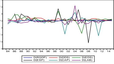
Figure 1: Stationarity of Variables at First Difference Figure 1 depicts a graphical analysis of
variables (LRGDP, LDDS, LEDS, LDSP, and LESP) when differenced the first time. The variables move around the zero mean which indicates that they are stationary at first difference.
Johansen Co-integration test
The co-integration test was carried out using the Johansen technique also using the Eviews 9 software package and it produced the following results:
Table 4: Test for Johansen Co-integration Using Trace Statistic Hypothesized
No. of CE(s)
Eigen Value Trace Statistic 0.05 Critical Value Prob.** None * 0.875852 145.9112 95.75366 0.0000 At most 1 * 0.730662 85.40894 69.81889 0.0017 At most 2 0.530403 47.36712 47.85613 0.0555 At most 3 0.366488 25.44657 29.79707 0.1461 At most 4 0.333111 12.20876 15.49471 0.1472 Source: Author‟s Compilation (2018)
From Table 4, the trace indicates two (2) co-integrating equation at 5 percent level. *
denotes rejection of the hypothesis at the 5 percent level.
Table 5: Test for Johansen Co-integration Using Max-Eigen Value Hypothesized
No. of CE(s)
Eigen Value Max-Eigen Statistic 0.05 Critical Value Prob** None * 0.875852 60.50222 40.07757 0.0001 At most 1 * 0.730662 38.04182 33.87687 0.0150 At most 2 0.530403 21.92055 27.58434 0.2245 At most 3 0.366488 13.23781 21.13162 0.4306 At most 4 0.333111 11.74880 14.26460 0.1204 Source: Author‟s Compilation (2018)
-4 -3 -2 -1 0 1 2 3 84 86 88 90 92 94 96 98 00 02 04 06 08 10 12 14 D(RGDP) D(DDS) D(EDS)
74 From Table 5, the Max-Eigen value indicates two (2) co-integrating equation at
5 percent level. * denotes rejection of the hypothesis at the 5 percent level.
Table 6: Long run Normalized Co-integration Estimates
RGDP DDS EDS ESP CAP LAB
1.000000 -0.416196 0.995066 -0.517354 0.371368 0.649168 (0.02836) (0.07556) (0.05479) (0.06473) (0.11360) Source: Author‟s Compilation (2018)
Table 6 shows the normalized co-integration co-efficient with the standard error in -parenthesis. A negative relationship exists between LRGDP and LDDS. A positive relationship exists between LRGDP and LEDS. A negative relationship exists between LRGDP and LESP. A positive relationship exists between LRGDP and LCAP. A positive relationship exists between LRGDP and LLAB.
Lag Length Selection for ECM
The Lag length selection criteria is to help to know the number lag value of the independent and dependent variable to be included in the ECM model. Table 7 shows that one (1) lag of both the independent and dependent variable will be included in the ECM model and this is selcetd by LR, FPE, SC and HQ criteria.
Table 7: VAR Lag Order Selection Criteria
Lag LogL LR FPE AIC SC HQ
0 -145.3594 NA 0.001376 10.43858 10.72147 10.52717 1 31.79095 268.7798* 8.63e-08* 0.704072 2.684294*
1.324253 * 2 72.49848 44.91865 8.88e-08 0.379415* 4.056969 1.531179 * indicates lag order selected by the criterion
LR:sequential modified LR test statistic (each test at 5% level) FPE: Final prediction error
AIC: Kaike information criterion SC: Schwarz information criterion
HQ: Hannan-Quinn information criterion
Source: Author‟s Compilation (2018)
Military Regime ECM 1 model result The result of ECM model in the Military regime (1983 - 1998) after the elimination of relatively insignificant
parameters in the overparameterized model are presented in Table 8.
75
Table 8: Result of ECM model in the Military regime (1983 - 1998) Parsimous Military
Dependent Variable: D(RGDP) Sample (adjusted): 1987 1998
Included observations: 12 after adjustments
Variable Coefficient Std. Error t-Statistic Prob.
C 0.036311 0.016868 2.152644 0.1642 D(DDS) 0.049204 0.065281 0.753722 0.5297 D(EDS) -0.046167 0.098692 -0.467785 0.6860 D(ESP) 0.064371 0.034559 1.862664 0.2035 D(CAP) -0.001289 0.134182 -0.009604 0.9932 D(DDS(-1)) -0.071547 0.042995 -1.664081 0.2380 D(EDS(-1)) -0.027941 0.048747 -0.573178 0.6244 D(ESP(-1)) 0.033295 0.053549 0.621766 0.5975 D(CAP(-1)) -0.064913 0.126527 -0.513039 0.6590 ECT(-1) -0.063401 0.696842 -0.090984 0.9358 R-squared 0.904528 Mean dependent var 0.031856 Adjusted R-squared 0.474905 S.D. dependent var 0.032949 F-statistic 2.105400 Durbin-Watson stat 2.140387 Prob(F-statistic) 0.363352
Source: Author‟s Compilation (2018) The result in Table 8 shows that the value of coefficient of determination (R2) is 0.904528. It implies that the exogenous variables in the ECM equation EDS, DDS, ESP, CAP and LAB explain over 90.45% of the systematic variations in RGDP while the remaining variation in GDP is caused by factors outside the model captured in the stochastic term (μ). Taking into consideration the degree of freedom, the Adjusted R2 dips down a little to 0.474905. This confirms the goodness of fit of the model. The Durbin Watson statistic of
2.140387 shows that the model is free from autocorrelation problem. The ECM term also has the correct sign of negative meaning that about 6.3% of the errors are corrected yearly.
Civilian Regime ECM 2 model result The result of ECM model in the Civilian regime (1999 - 2015) after the elimination of relatively insignificant parameters in the overparameterized model is presented in Table 9.
76
Table 9: Result of ECM 2 model in the Civilian Regime (1999 - 2015) Parsimous Model for Civilian Regime
Variable Coefficient Std. Error t-Statistic Prob.
C 0.045876 0.027536 1.666042 0.1152 D(DDS) -0.015601 0.065591 -0.237849 0.8150 D(EDS) -0.010420 0.015575 -0.669029 0.5130 D(ESP) 0.000820 0.009861 0.083143 0.9348 D(CAP) 0.008090 0.013395 0.604007 0.5543 D(LAB) -0.005365 0.019427 -0.276143 0.7860 D(RGDP(-1)) 0.437337 0.291570 1.499937 0.1531 D(DDS(-1)) -0.069418 0.047274 -1.468421 0.1614 D(EDS(-1)) 0.006807 0.015918 0.427636 0.6746 D(ESP(-1)) -0.002334 0.008584 -0.271947 0.7891 D(CAP(-1)) -0.011789 0.013818 -0.853193 0.4061 D(LAB(-1)) -0.008933 0.020814 -0.429201 0.6735 ECT(-1) 0.024874 0.113354 0.219438 0.8291
R-squared 0.440982 Mean dependent var 0.052092
Adjusted R-squared 0.021719 S.D. dependent var 0.034950
S.E. of regression 0.034569 Akaike info criterion -3.589883
Sum squared resid 0.019120 Schwarz criterion -2.976957
Log likelihood 65.05330 Hannan-Quinn criter. -3.397922
F-statistic 1.051802 Durbin-Watson stat 2.043495
Prob(F-statistic) 0.453064
Source: Author‟s Compilation (2018)
The result in Table 9 shows that the value of coefficient of determination (R2) is 0.440982. This shows that the exogenous variables in the ECM 2 equation EDS, DDS, ESP, CAP and LAB explain over 44.010% of the systematic variations in RGDP while the remaining variation in GDP are caused by factors outside the model captured in the stochastic term (μ). The Durbin Watson statistic of 2.043495 also buttress the reliability of the model.
Pooled ECM 3 Model Result:
Table 10: The result of Parsimonious model of the whole economy
Variable Coefficient Std. Error t-Statistic Prob.
C -0.107232 0.042805 -2.505148 0.0873 D(DDS) 0.281469 0.091955 3.060937 0.0550 D(EDS) -0.024072 0.013927 -1.728380 0.1824 D(ESP) 0.025938 0.014596 1.777018 0.1736 D(CAP) 0.049325 0.018956 2.602055 0.0802 D(LAB) 0.035434 0.014551 2.435199 0.0929 D(RGDP(-1)) 1.517298 0.358414 4.233368 0.0241 D(DDS(-1)) 0.250600 0.153562 1.631912 0.2012 D(EDS(-1)) -0.020045 0.012424 -1.613416 0.2051 D(CAP(-1)) -0.013369 0.009104 -1.468585 0.2383 D(LAB(-1)) -0.005631 0.015296 -0.368137 0.7372 ECT(-1) -1.671128 0.477730 -3.498058 0.0395
77
R-squared 0.890749 Mean dependent var 0.071298
Adjusted R-squared 0.490164 S.D. dependent var 0.026204 S.E. of regression 0.018710 Akaike info criterion -5.128920 Sum squared resid 0.001050 Schwarz criterion -4.562480 Log likelihood 50.46690 Hannan-Quinn criter. -5.134954 F-statistic 2.223617 Durbin-Watson stat 2.496110 Prob(F-statistic) 0.277460
Source: Author‟s Compilation (2018)
The Pooled ECM model result as shown in Table 10 yields R-square of 0.890749 and Durbin Watson statistics of appropriately 2. These statistics attests to the good fit and reliability of the model. The exogenous variables in the ECM equation EDS, DDS, ESP, CAP and LAB explain over 89.07% of the systematic variations in RGDP while the remaining variation in GDP are caused by factors outside the model captured in the stochastic term (μ). Taking into consideration the degree of freedom, the Adjusted R2 dips down a little to 0.490164.
Consistent with the main objective of this study, domestic debt service as observed in Table 10 is seen to have a positive effect on economic growth at 10% level of significance when the two regimes
are pooled into one. This implies that a 1% increase in DDS will lead to a corresponding 28.1 % increase in economic growth. This is in line with the findings of Ijeoma (2013) and Adesola et al. (2015) that debts channelled towards developmental projects create positive effects for the economy. Similarly, CAP and LAB are significant at 10% alpha level with both having a positive effect on economic growth. However, Tables 8 and 9 for the military and civilian regimes respectively show that DDS, EDS and ESP do not have any significant effect on the economy. Model Diagnostics
Residual Test: Jarque Bera test for normality of residual accept the null hypothesis that the residual is normally distributed.
Figure 4.2 Test for Normallity of Residual Source: Author‟s Compilation (2018) 0 1 2 3 4 5 6 -0.06 -0.04 -0.02 0.00 0.02 0.04 Series: Residuals Sample 1987 2015 Observations 29 Mean -5.74e-18 Median 0.003765 Maximum 0.049651 Minimum -0.055194 Std. Dev. 0.026132 Skewness -0.207738 Kurtosis 2.343605 Jarque-Bera 0.729199 Probability 0.694475
78 So also was the Ljung-Box Q-statistics test for autocorrelation. The test shown in Appendix A indicates that there is no autocorrelation in the residual.
Heteroscedasticity Test: As shown in Appendix B, Breusch-Pagan Godfrey test with null hypothesis of no Heteroscedasticity is accepted.
The result in the ECM 1 model shows that the impact of debt structure and other variables on the Real Gross Domestic Product are more impactful during the military when coefficient of determination (R2) is 90.45% while the adjusted R2 was very low with the value of 47.49%. The ECM 2 for civilian regime also shows that the model with coefficient of determination (R2) is 44.09% while the adjusted R2 is low at 2.17%. Finally, the pooled result of the whole economy was showing that coefficient of determination (R2) is 89.07% while the adjusted R2 49.01%. This indicates the model reveals that RGDP was more impactful during the military than in the civilian regime and was also impactful on the whole put together.
Furthermore, F-statistical value of ECM 3 is (2.223617) which is statistically significant at the 5% level going by its probability value of 0.277460. This implies that EDS, DDS, ESP, CAP and LAB taken together are jointly significant in explaining and are also good predictors of the dependent variable, GDPPC. The Durbin-Watson statistic of 2.496110 is indicative of the absence of positive serial autocorrelation in the model. The coefficient of the ECT (-1) is significant with the appropriate negative sign, indicating that the adjustment is in the right direction to restore the long-run relationship. Its coefficient of -1.671128 means that the present value in RGDP adjusts rapidly to previous changes in EDS, DDS, ESP, CAP and LAB specifically by about 167%. Unit root test was carried out using the Augmented Dickey-Fuller (ADF)
test and Phillip Perron (PP) test. The tests revealed that none of the variables were stationary at level form but all the variables became stationary at first difference. integration test using the Johansen Co-integration technique was also carried out. The result from the test showed that LRGDP, LDDS, LEDS, LDSP, LESP, LCAP, LLAB are integrated of order one i.e they became stable after the first difference. The model diagnostic tests indicate normality of residual and accepted the null hypothesis that the residual is normally distributed. The Ljung-Box Q-statistics test for autocorrelation shows that there is no autocorrelation in the residual while the heteroscedasticity test of Breusch-Pagan Godfrey shows that the null hypothesis of no heteroscedasticity was accepted. Conclusion and Recommendations
This study examined the impact of public debt and its management on the economic growth of Nigeria taking into consideration the influences of military and civilian rules. This was done by examining the short and long run relationship between public debt management and economic growth using econometric analysis which included the test for stationarity using Augumented Dickey Fuller (ADF) and Philip Perron (PP) tests for co-integration using Johansen co-integration test and the error correction model using system of equation with dummy variable to test the hypothesis of this research.
The analysis carried out revealed that a significant long run relationship exist between Real Gross Domestic Product (LRGDP), Domestic Debt Stock (LDDS), External Debt Stock (LEDS), External Debt Service Payment (LESP), Capital formation (LCAP) and Labour (LLAB) during the military regime and low a little level of significant during the civilian regime. However, there was a and significant relationship during the period under
79 consideration as a whole. This implies that most of the public borrowings and debt management carried out within the period of civilian was rather too large. There should be checks as to the way different states are borrowing. This is evident in the test of mean differences. Furthermore, borrowings should be growth-oriented. These findings are in line with Sunday et al (2016) who also are of a conclusion that there was a “little significant impact of external and domestic debt on the economic growth in Nigeria during the period under consideration” (pg. 142). While a significant relationship exist between the military and civilian rules, it witnessed an increase in Nigeria‟s public debt burden which gives a negative impact on the economic growth of the country.
Based on the above findings, the following recommendations were given:
1. Public borrowing (internal and external) should be based on developmental projects to be executed and should also be invested on productive sectors of the economy that would stimulate growth in the long-run.
2. The Debt Management Office (DMO) should set maximum limit for loans that could be allowed for state and federal governments based on certain required criteria especially to avoid reckless debt in the civilian regime.
3. Adequate servicing of debts should be done and the debt should not be allowed to pass a maximum limit (e.g. debt-to-GDP ratio of less than 20% should be sustained) in order to avoid debt overhang.
References
Abula, M. & Mordecai B. D. (2016). The Impact of Public Debt on Economic Development of Nigeria. Asian
Research Journal of Arts & Social Sciences, 1 (1), 1-16.
Adesola, I., Olaide, A., Adeola, B., Bright, I. & Victor, O., (2015). Nigerian Debt Portfolio and Its Implication on Economic Growth. Journal of
Economics and Sustainable
Development, 6 (18), 87-99.
Ajayi, L. & Oke, M. (2012). Effect of External Debt on Economic Growth and Development of Nigeria. International Journal of Business and Social Science, 3 (12), 297-304. Anochie, U. C., & Ude, D. K., (2015).
Nigerian‟s Management of the External Debt: Issues, Challenges and prospects. International Journal of Financial Economics, 4(4), 195-208.
Arit, E. N., (2013). Exploring The Nexus Between External Debt Management And Economic Growth. International Journal of Economics Research, 4 (2), 43-65.
Barbara, Eric, & Colleen. (2015). Nigeria country report.
Central Bank of Nigeria. (2015). Statiscal Bulletin for various years.
Debt Management Office. (2017). National Debt Management Framework (2013 to 2017).
Debt Management Office. (2015). Annual Report and Statement of Account for various years
Debt Management Office . (2016). Retrieved from Debt Management Office Nigeria. http://wwwdmo.org
Dereje, A. E. & Joakim, P. (2013). The Effect of External Debt On Economic growth – A panel data analysis on the relationship between external debt and economic growth.Södertörns högskola | Department of economics, Magisteruppsats 30 hp | Vårterminen Ijeoma, N. B. (2013). An Empirical Analysis of the Impact of Debt on the Nigerian Economy . International Journal of Arts and Humanities, 2 (3), 165-191.
80 International Monetary Fund, & World Bank.
(2001). Guidelines for Public Debt Management.
International Monetary Fund, & World Bank. (2014). Revised Guidelines For Public Debt Management.
Investopedia. (2016, December). Retrieved from http://www.investopedia.com Madu. A. Y., Abbo. U., Rohana.Y., &
Suyatno.L. (2015). The Political Economy of External Debt Management in Nigeria: Strategies, Issues and Challenges. Australian Journal of Basic and Applied Sciences, 23-30.
Tajudeen, E. (2012). Public Debt and Economic Growth in Nigeria: Evidence from Granger Causality. American Journal of Economics, 2 (6), 101-106.
Tomás, J. B. & Sundararajan, V., (2008). Public Debt Management in Developing Countries: Key Policy, Institutional, and Operational issues.
Workshop on Debt, Finance and Emerging Issues.
Udeh, S., Ugwu, J. & Onwuka, I. (2018). External Debt And Economic Growth: The Nigeria Experience. European Journal of Accounting Auditing and Finance Research, 4 (2), 33-48.
Yusuf, B., Idowu, K., Okunnu, M. & Adeyemi, O. (2010). Debt management and economic growth in Nigeria : performance, challenges and responsibilities. Manager, 12, 31-39
81 Appendix: A
Ljung-Box Q-statistics test for autocorrelation: The test also shows that there is no autocorrelation in the residual up to lag 36.
Q-statistic probabilities adjusted for 13 dynamic regressors
Autocorrelation Partial Correlation AC PAC Q-Stat Prob* . |* . | . |* . | 1 0.076 0.076 0.1777 0.673 . | . | . | . | 2 -0.054 -0.060 0.2727 0.873 . |* . | . |* . | 3 0.187 0.198 1.4528 0.693 . *| . | . *| . | 4 -0.150 -0.195 2.2364 0.692 . *| . | . | . | 5 -0.119 -0.061 2.7511 0.738 . |* . | . |* . | 6 0.116 0.080 3.2627 0.775 . | . | . | . | 7 -0.057 -0.028 3.3923 0.846 .**| . | .**| . | 8 -0.236 -0.226 5.7315 0.677 . | . | . *| . | 9 -0.046 -0.077 5.8255 0.757 ***| . | ***| . | 10 -0.360 -0.386 11.875 0.294 . *| . | . | . | 11 -0.178 -0.054 13.444 0.265 . | . | . *| . | 12 0.046 -0.092 13.553 0.330 . *| . | . *| . | 13 -0.188 -0.204 15.530 0.275 . |* . | . |* . | 14 0.125 0.100 16.460 0.286 . |* . | . | . | 15 0.139 -0.039 17.701 0.279 . | . | . | . | 16 -0.040 -0.009 17.816 0.335 . | . | . | . | 17 0.050 -0.057 18.008 0.388 . |* . | . | . | 18 0.187 -0.007 20.943 0.282 . *| . | . *| . | 19 -0.074 -0.166 21.451 0.312 . | . | . *| . | 20 0.043 -0.117 21.643 0.360 . |* . | . *| . | 21 0.200 -0.068 26.439 0.190 . *| . | . *| . | 22 -0.103 -0.107 27.917 0.178 . | . | . *| . | 23 -0.031 -0.183 28.074 0.213 . | . | . | . | 24 0.035 -0.053 28.332 0.246 . | . | . |* . | 25 0.016 0.116 28.401 0.290 . | . | . | . | 26 -0.019 -0.036 28.550 0.332 . | . | . *| . | 27 -0.064 -0.140 31.981 0.233 *Probabilities may not be valid for this equation specification.
Appendix: B
Heteroscedasticity Test: As shown in the table below, Breusch-Pagan Godfrey test with null hypothesis of Heteroscedasticity is accepted.
Heteroskedasticity Test: Breusch-Pagan-Godfrey
F-statistic 0.185614 Prob. F(13,14) 0.9978 Obs*R-squared 4.116464 Prob. Chi-Square(13) 0.9899 Scaled explained SS 1.162293 Prob. Chi-Square(13) 1.0000 Source: Author’s Compilation