Outi Väisänen
Multichannel EEG Methods to Improve the Spatial
Resolution of Cortical Potential Distribution and the
Signal Quality of Deep Brain Sources
Tampere University of Technology. Publication 741
Outi Väisänen
Multichannel EEG Methods to Improve the Spatial
Resolution of Cortical Potential Distribution and the
Signal Quality of Deep Brain Sources
Thesis for the degree of Doctor of Technology to be presented with due permission for public examination and criticism in Rakennustalo Building, Auditorium RG202, at Tampere University of Technology, on the 13th of June 2008, at 12 noon.
Tampereen teknillinen yliopisto - Tampere University of Technology Tampere 2008
ISBN 978-952-15-1986-4 (printed) ISBN 978-952-15-1999-4 (PDF) ISSN 1459-2045
Electroencephalography (EEG) is a convenient technique for studying the function of the brain non‐invasively from the surface of the scalp. The greatest advantages of EEG are its temporal resolution on a millisecond scale and its affordability compared to other non‐ invasive techniques employed to register brain activity. The development in amplifier technology, computerized signal processing methods and modern EEG caps make the application of multichannel EEG systems a feasible objective. Nowadays measurement systems of up to 256 electrodes and over are available. It is thus important to evaluate the benefits obtained with the multichannel systems when different functions of the brain are being studied.
In this thesis two opposite applications of multichannel EEG are investigated. The first of these deals with superficial sources and concerns improving the spatial resolution of inverse cortical potential distribution. The other application concerns the modification of the measurement sensitivity distributions of EEG leads to improve the signal‐to‐noise ratio (SNR) of signals generated deep within the brain.
When studying the spatial resolution of cortical potential distribution, special attention was given to an examination of the effect of measurement noise and relative skull resistivity on the estimation of accuracy of the inverse solution. A three‐layer spherical head model was applied with new realistic estimates for skull resistivity. The measurement noise levels were estimated in realistic measurement environments, bearing in mind that when the cortical potential distribution is studied as a solution of the inverse problem, the entire brain activity is considered as the desired signal. The results of the theoretical evaluation show that with the new realistic estimates for relative skull resistivity, the application of up to 128 ‐ 256 electrodes improves the spatial resolution of cortical potential distribution.
To improve the SNR of signals generated by deep EEG sources, multielectrode EEG leads were developed. Theoretically a multielectrode EEG lead consists of two terminals, which are both connected through a resistor network to several electrodes on the surface of the scalp. Reciprocity and lead field theorems were applied to modify the sensitivity distribution of a multielectrode lead to be optimal for deep brain sources. The results of preliminary experimental evaluation conducted by studying brainstem auditory evoked potentials show that with a multielectrode EEG lead consisting of 114 electrodes, it is sufficient to average 45 % of the number of epochs needed with bipolar leads to obtain a similar SNR. The results of the theoretical study demonstrate that further improvements can be obtained by such steps as optimizing the electrode positions.
ACKNOWLEDGEMENTS
The work for the thesis was carried out at the Ragnar Granit Institute, Department of Electrical Engineering, Tampere University of Technology. Due to structural reform at Tampere University of Technology, the work was finalized at the new Department of Biomedical Engineering.
I wish to express my gratitude to my supervisor, Professor Jaakko Malmivuo, PhD, for his guidance throughout this research; his expertise in bioelectromagnetism has been invaluable. I would also like to thank the head of the department, Professor Jari Hyttinen, PhD, for his guidance, especially during the initial stages. His contribution, together with that of Päivi Laarne, PhD, was inspirational for my investigations into the field of modelling.
I would also like to thank Docent Ville Jäntti, MD, for his guidance in planning the experimental EEG measurements. I also gratefully acknowledge the help of Pasi Kauppinen, PhD, and Riina Meriläinen‐Juurikka, BEng, for setting up the multichannel EEG equipment for the measurements. I am also indebted to all my colleagues at Ragnar Granit Institute and especially all the volunteers who so kindly gave their time for the lengthy measurement sessions.
I wish to thank Sylvain Baillet, PhD, (Pierre & Marie Curie University, France), Geertjan Huiskamp, PhD, (University Medical Center Utrecht, The Netherlands) and Bart Vanrumste, Dr Ir, (Katholieke Universiteit Leuven, Belgium) for their constructive criticism and advice as examiners of this thesis. I also thank Alan Thompson, MPhil, for carefully revising the English of my thesis.
The financial support of The Graduate School of Tampere University of Technology, The Academy of Finland, The Finnish Cultural Foundation, The Wihuri Foundation and The Ragnar Granit Foundation is gratefully acknowledged.
I would also like to thank my parents and sister for all their support. Finally, my heartfelt gratitude goes to my husband Juho. He not only helped me strike a balance between work and leisure when I most needed it, but also as my colleague, contributed to my research.
Tampere, May 2008
ABSTRACT ... i
ACKNOWLEDGEMENTS ... iii
LIST OF ORIGINAL PUBLICATIONS ... vii
AUTHOR’S CONTRIBUTION ... viii
LIST OF ABBREVIATIONS ... ix
LIST OF SYMBOLS ... x
1 INTRODUCTION ... 1
2 OBJECTIVES OF THE STUDY ... 3
3 REVIEW OF THE LITERATURE AND THEORETICAL BACKGROUND ... 5
3.1 ELECTROENCEPHALOGRAPHY (EEG) ... 5
3.1.1 Properties of EEG ... 5
3.1.2 Genesis of EEG signals ... 6
3.1.3 EEG electrode systems ... 6
3.1.4 Noise in EEG measurements ... 8
3.1.5 SNR Improvement of EEG measurements ... 10
3.2 EEG INVERSE PROBLEMS ... 11
3.2.1 Definition of an EEG inverse problem ... 11
3.2.2 Discrete source localization methods ... 11
3.2.3 Source imaging methods ... 12
3.2.4 Formulation of the EEG inverse problem ... 14
3.2.5 Effect of noise in EEG inverse solutions ... 15
3.3 VOLUME CONDUCTOR MODELS ... 18
3.3.1 Properties of volume conductor models ... 18
3.3.2 Geometry of the model ... 18
3.3.3 Electrical properties of the model ... 20
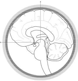
3.3.4 Skull resistivity ... 20
3.4 IMPROVEMENT OF THE SPATIAL RESOLUTION OF EEG ... 23
3.4.1 Spatial resolution of EEG ... 23
3.4.2 Distributed source models and cortical imaging ... 24
3.4.3 Number of EEG electrodes in improving spatial resolution ... 27
3.5 SENSITIVITY DISTRIBUTION OF EEG MEASUREMENT LEADS ... 30
3.5.1 Lead field and reciprocity theorem ... 30
3.5.2 Sensitivity distribution of two‐electrode EEG ... 32
3.5.3 Modifications of sensitivity distributions ... 32
4 MATERIALS AND METHODS ... 35
4.1 VOLUME CONDUCTOR MODEL... 35
4.2 EEG ELECTRODE SYSTEMS ... 35
4.3 SPATIAL RESOLUTION OF CORTICAL POTENTIAL DISTRIBUTION [I‐III] ... 36
4.3.1 Setting up the system of equations ... 36
4.3.2 Finite difference method ... 37
4.3.3 Analysis of the accuracy of cortical potential distribution ... 37
4.4 IMPROVED SIGNAL QUALITY OF DEEP EEG SOURCES [IV‐VII] ... 38
4.4.1 Synthesisation of multielectrode EEG leads ... 38
4.4.2 Sensitivity distribution analysis ... 40
4.4.3 Simulation study ... 40
5 RESULTS ... 43
5.1 SPATIAL RESOLUTION OF CORTICAL POTENTIAL DISTRIBUTION ... 43
5.1.1 Effect of measurement noise ... 43
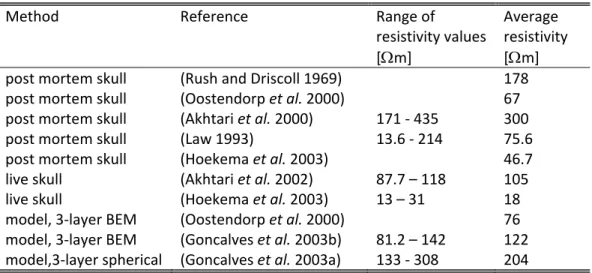
5.1.2 Estimation of the relative noise level ... 44
5.1.3 Effect of skull resistivity on the spatial resolution of cortical potential distribution ... 45
5.2 IMPROVED SIGNAL QUALITY OF DEEP EEG SOURCES ... 46
5.2.1 ROISR parameter in defining the specificity of an EEG lead ... 46
5.2.2 Effect of source depth on the specificity of two‐electrode EEG leads ... 46
5.2.3 Specificity of a multielectrode EEG leads for deep EEG sources ... 46
5.2.4 Improvement in SNR in a simulation study ... 48
5.2.5 Experimental evaluation of multielectrode EEG leads ... 48
6 DISCUSSION ... 51
6.1 MULTICHANNEL EEG ... 51
6.2 SPATIAL RESOLUTION OF CORTICAL POTENTIAL DISTRIBUTION ... 51
6.2.1 Measurement noise ... 51
6.2.2 Relative skull resistivity ... 52
6.2.3 Electrode density ... 53
6.2.4 TSVD in defining spatial resolution ... 54
6.2.5 Accuracy of the applied models ... 54
6.3 IMPROVED SIGNAL QUALITY OF DEEP EEG SOURCES ... 55
6.3.1 Specificity of EEG leads ... 55
6.3.2 Spatial averaging in multielectrode EEG leads ... 55
6.3.3 Feasibility of multielectrode EEG leads ... 56
6.3.4 Comparison to other SNR improvement methods ... 56
6.3.5 Comparison to beamformers ... 57
6.3.6 Future development of multielectrode leads ... 58
7 CONCLUSIONS ... 61
8 REFERENCES ... 63
LIST
OF
ORIGINAL
PUBLICATIONS
This thesis is based on the following publications, referred to in the text by Roman numerals.
I. Ryynänen O, Hyttinen J, Laarne P, and Malmivuo J. Effect of electrode density
and measurement noise on the spatial resolution of cortical potential distribution. IEEE Transactions on Biomedical Engineering, vol. 51, no. 9, pp. 1547‐1554, 2004.
II. Ryynänen O, Hyttinen J, Laarne P, and Malmivuo J. Effect of measurement
noise on the spatial resolution of EEG. Biomedizinische Technik, vol. 48, Supplement 2, pp. 94‐97, 2004.
III. Ryynänen O, Hyttinen J and Malmivuo J. Effect of measurement noise and
electrode density on the spatial resolution of cortical potential distribution with different resistivity values for the skull. IEEE Transactions on Biomedical
Engineering, vol. 53, no. 9, pp. 1851‐1858, 2006.
IV. Väisänen J, Väisänen O, Hyttinen J, and Malmivuo J. New Method for Analysing Sensitivity Distributions of Electroencephalography Measurements.
Medical & Biological Engineering & Computing, vol. 46, no. 2, pp. 101‐108, 2008.
V. Ryynänen O, Väisänen J, Hyttinen J, and Malmivuo J. Effect of source depth
on the specificity of bipolar EEG measurements. In the Proceedings of the
28th Annual International Conference of the IEEE Engineering in Medicine and
Biology Society, New York City, USA, 30.8.‐3.9.2006 pp. 1110‐1113.
VI. Väisänen O and Malmivuo J. Improving the SNR of EEG generated by deep
sources with multielectrode leads. Journal of Physiology ‐ Paris, submitted.
VII. Väisänen O and Malmivuo J. Improved Detection of Deep Sources with
Weighted Multielectrode EEG Leads. In the Proceedings of the 29th Annual
International Conference of the IEEE Engineering in Medicine and Biology
Society, Lyon, France, 23.‐26.8.2007 pp. 5194‐5197.
Outi Ryynänen is the maiden name of Outi Väisänen
AUTHOR’S
CONTRIBUTION
Publications I – III concern the spatial resolution of cortical potential distribution. Professor Jari Hyttinen originally presented the idea of studying the effect of electrode number on the accuracy of the estimation of the cortical potential distributions. The author has otherwise designed the studies, implemented the method (excluding the programming of the numerical method) and prepared the results. The author has also written the papers, while receiving comments from the co‐authors.
As co‐author of Publication IV, the author has been involved in designing the new parameter also for the purposes of Publications V‐VII. The author has also participated in designing the experimental measurements. The methods were implemented and the results were prepared by Juho Väisänen. The author also participated in the writing of the manuscript. In Publication V, the author implemented the methods, prepared the results and wrote the paper.
Publications VI and VII concern the development of the multielectrode lead method. The original idea of modifying the lead field with multichannel EEG to be optimal for deep sources was proposed by Professor Jaakko Malmivuo. The author has designed the studies, implemented the methods including the experimental measurements and prepared the results. The work was conducted under the supervision of the co‐author. The author has also written the papers, while receiving comments from the co‐author.
LIST
OF
ABBREVIATIONS
AC alternating current
BAEP brainstem auditory evoked potential BEM boundary element method
CIT cortical imaging technique CSF cerebrospinal fluid CT computed tomography DC direct current ECG electrocardiography ECoG electrocorticography EEG electroencephalography
EIT electrical impedance tomography EMG electromyography
EOG electro‐oculography EP evoked potential
FDM finite difference method FEM finite element method
fMRI functional magnetic resonance imaging GWN Gaussian white noise
HSV half‐sensitivity volume
LCMV linearly constrained minimum variance
LORETA low‐resolution brain electromagnetic tomography MEG magnetoencephalography
MR magnetic resonance
MUSIC multiple signal classification NL relative noise level
PET positron emission tomography RBV reconstructable basis vector RMS root mean square
ROI region of interest
ROISR region of interest sensitivity ratio SEP somatosensory evoked potential SNR signal‐to‐noise ratio
SPECT single proton emission computed tomography SVD singular value decomposition
TSVD truncated singular value decomposition VEP visual evoked potential
LIST
OF
SYMBOLS
A forward transfer matrix
A+ pseudoinverse of matrix A
b vector of EEG potentials
cL lead vector
e measurement error vector
Ir reciprocal current
Ji impressed current density
JL lead field current density
n(t) noise signal K(xC,xS) kernel p source dipole s(t) desired signal SC cortical surface SS scalp surface t time
ui left singular vector vi right singular vector uiTb Fourier coefficient of b U left singular matrix viTx Fourier coefficient of x V right singular matrix
V volume
VL measured potential wi weight of unipolar lead
x source vector
x+ least‐squares solution
xC location on the cortical surface
xS location on the scalp surface
x(t) noise‐contaminated signal
σ conductivity
σi singular value
Σ singular value matrix τ error level
φS(xS) scalp surface potential φC(xC) cortical surface potential
Electroencephalography (EEG) is a standard method in neurophysiology to study the function of the brain. Both spontaneous activity and evoked potentials (EP) can be measured with electrodes attached to the surface of the scalp. EEG has a wide range of clinical applications ranging from diagnosis of epilepsy and brain tumours to the analysis of sleep and the depth of anaesthesia. Measured evoked potentials, on the other hand, can be used in diagnosis of central nervous system diseases and in studies concerning the cognitive processes. (Nunez and Srinivasan 2006)
In addition to EEG, there are also other non‐invasive techniques that can be used to monitor brain function. These include magnetoencephalography (MEG), functional magnetic resonance imaging (fMRI), positron emission tomography (PET) and single photon emission computed tomography (SPECT) (Gevins et al. 1990; Wikswo et al. 1993; Michel et al. 2004). EEG and MEG measure the electric and magnetic field, respectively, generated by the electrical activity of the brain, while fMRI, PET and SPECT measure the hemodynamic response (Shibasaki 2008). These methods differ in their temporal and spatial properties. The temporal resolution below the millisecond scale of EEG and MEG is superior to the other imaging modalities, whereas the spatial resolution of fMRI and PET is superior to that of conventional EEG and MEG.
It has been widely acknowledged that the spatial resolution of the traditional 10‐20 – electrode system is not sufficient for modern brain research (Gevins et al. 1995; Gevins et
al. 1999; Babiloni et al. 2001b; Michel et al. 2004). If the spatial resolution is poor, localization of the complex distribution of the electrical activation is difficult. Accurate localization is important for studying the fine topography related, for example, to higher order cognitive brain functions and seizure onsets as well as in planning tumour and epilepsy surgery. (Pohlmeier et al. 1997; Wang and He 1998; Gevins et al. 1999)
The spatial resolution of EEG is affected by blurring caused by volume conductor effects, the largest being the effect of the low conducting skull. A volume conductor model of the head can be constructed to study the effects of different tissues on the volume conduction. The most important characteristics of a head model are its geometrical shape and the resistivities assigned to different tissues. For a long time it was assumed that the resistivity of the skull is 80 times that of scalp and brain (Rush and Driscoll 1968, 1969),
but during the last decade it has been shown that this value is greatly overestimated (Oostendorp et al. 2000; Akhtari et al. 2002; Hoekema et al. 2003).
The spatial resolution of EEG can be improved by first increasing the number of measurement electrodes, and secondly, by applying a spatial enhancement method to reduce the effect of blurring. The multichannel EEG is nowadays convenient to apply because of the improvements in EEG amplifier technology and computerized signal processing methods. The Laplacian derivation (Hjorth 1975) was the first of the spatial enhancement methods to be introduced. It is a fairly simple method, which does not necessarily require the construction of a volume conductor model. Another possibility is to improve the spatial resolution by solving the inverse cortical source distribution. These methods are called source imaging methods and they require the construction of a volume conductor model. The spatial resolution is improved because the effect of the low conducting skull is taken into account. Examples of such methods are the cortical imaging technique (Kearfott et al. 1991; Sidman et al. 1992; Babiloni et al. 1997b; Wang and He 1998; Zhang et al. 2006a) and the deblurring method (Gevins et al. 1991; Le and Gevins 1993; Gevins et al. 1994; Gevins et al. 1999).
Most of the EEG signal measured from the scalp surface with two‐electrode EEG leads is generated by cortical activity. When evoked potentials generated at deeper structures are measured, a typical means to improve the signal‐to‐noise ratio (SNR) is to average a large number, even thousands, of epochs. Beamformer methods have also been introduced to enhance the signals generated at different depths within the brain. Beamformers act as spatial filters. Beamformers are usually applied to source localization, but their basis is in passing the signals generated in the target region within the brain (Van Veen et al. 1997; Ward et al. 1999). Application of a large number of electrodes provides a means for optimizing the properties of the spatial filters.
An illustrative and simple way to study the sensitivity of different measurement leads is provided by the reciprocity and lead field theorems (Malmivuo and Plonsey 1995). The lead field analysis reveals that the sensitivity of two‐electrode EEG leads is concentrated on the cortex (Malmivuo et al. 1997). The number of electrodes in both terminals of the lead can be increased to modify the sensitivity distributions. This method was introduced by McFee and Johnston (1954a), who modified electrocardiography (ECG) leads. With such multielectrode leads, it is possible to optimize the sensitivity distribution to be specific to sources at the target region, even those located deep within the brain.
2
OBJECTIVES
OF
THE
STUDY
This thesis concentrates on two main topics, both of which show potential to benefit from the application of multichannel EEG. These two applications represent contrasting approaches to the application of a large number of electrodes on the surface of the scalp; in the first of these the focus is on cortical sources, whereas in the second, it is on the deep EEG sources.
The first main topic is devoted to studying the spatial resolution of cortical potential distribution. The purpose is to theoretically define, independent of the underlying source pattern, how many electrodes are needed to obtain the highest possible spatial resolution of the inverse cortical potential distribution. The effect of measurement noise plays the most important role in defining a sufficient number of electrodes. The effect of the widely debated resistivity of the skull was also studied. In detail, the objectives of this first topic are as follows:
to study the effect of EEG electrode density on the spatial resolution of cortical potential distribution in the presence of measurement noise [I ‐ III]
to study the effect of skull resistivity on the spatial resolution of cortical potential distribution [III]
The second main topic concerns the development of new measurement leads to improve the SNR of EEG signals generated deep in the brain. For this purpose weighted multielectrode leads consisting of a large number of measurement electrodes were developed. The method is based on modifying the sensitivity distribution with the aid of the lead field theory. New parameters to describe the specificity of measurement sensitivity were also derived. In detail, the objectives of the second topic are as follows:
to study the specificity of different EEG leads to detect signals generated at different depths within the brain [IV ‐ V]
to develop weighted multielectrode EEG leads to improve the SNR of EEG generated by sources located deep in the brain [VI ‐ VII]
3.1
Electroencephalography
(EEG)
3.1.1 Properties of EEG
The first report on the measurement of the electrical activity of the brain was written in 1875 by British physician Richard Caton (1875), who measured the exposed brains of experimental animals. The first human EEG measurement was made by German neuropsychiatrist Hans Berger in 1924. One of the subjects reported in his first paper on human EEG (Berger 1929) was the existence of alpha rhythm. During the 1930s he published several other findings on human EEG related to different conditions. The first evoked potential studies were reported by George D. Dawson (1951), who stimulated electrically the ulnar nerve and measured the resulting evoked potentials. (Niedermeyer 2005b)
The typical clinically relevant frequency band of EEG is from 0.1 to 100 Hz. Sometimes a stricter band from 0.3 to 70 Hz is considered relevant. Amplitudes measured from the surface of the cortex can vary between 500 and 1500 µVpp. The amplitudes are attenuated considerably when they are volume‐conducted to the surface of the scalp. The amplitude of EEG measured from the scalp surface varies typically between 10 and 100 µVpp. In adults the maximum amplitudes are typically below 50 µVpp. The measured
amplitudes are also affected by the location of the electrodes and by the interelectrode distance. (Niedermeyer 2005a)
EEG oscillations are not restricted to the above mentioned frequency band. So‐called ultraslow EEG activity has a frequency band from DC to 0.3 Hz. EEG oscillations with higher frequencies than 100 Hz can also be measured. Curio (2005) refers to the high‐ frequency EEG oscillations between 400 and 1000 Hz by the term “ultrafast EEG”. Ultrafast EEG includes, for example, so‐called σ‐bursts which overlap the early somatosensory evoked potential (SEP) components. These bursts have generators both deep in the brain and on the cortex and they have a frequency around 600 Hz. The brainstem auditory evoked potentials (BAEP) are also an example of high‐frequency
oscillations (Nuwer et al. 1994). The high‐frequency oscillations have typically extremely low amplitudes.
EEG is characterised by good temporal resolution on a sub‐millisecond scale, but the spatial resolution of conventional EEG is poor. The spatial resolution is affected by blurring, which occurs as the EEG signals are volume‐conducted through the different tissues of the head. The spatial resolution of EEG can be improved by increasing the number of measurement electrodes and by applying a spatial enhancement method to reduce the effect of blurring.
3.1.2 Genesis of EEG signals
EEG recorded from the surface of the scalp is mainly generated by the synchronous activity of populations of neurons on the cerebral cortex. The main generators of EEG are the postsynaptic potentials in the dendrites of large pyramidal neurons. These neurons are highly interconnected and approximately 85 % percent of all cortical neurons are these pyramidal cells oriented parallel to each other and perpendicular to the local cortical surface (Nunez and Srinivasan 2006). As several neurons activate synchronously through superposition, they generate such a dipole moment that results in a measurable potential difference on the surface of the scalp. According to Nunez and Srinivasan (2006) approximately 6 cm2 of the cortical gyri tissue needs to activate synchronously to produce such measurable potentials at the scalp surface that can be detected without averaging. (Lopes da Silva and Van Rotterdam 2005; Nunez and Srinivasan 2006)
Evoked potentials are generated as a response to given stimuli. The stimuli can be sensory, motor, or cognitive. The evoked responses measured from the surface of the scalp have such a low signal level that averaging, for example, is needed to reduce the effect of noise. Evoked potentials generated in the brainstem can also generate measurable potentials on the surface of the scalp. These have extremely low SNR, and thus, averaging of even thousands of epochs is needed to reduce the effect of noise. An example of such EPs is the BAEPs, which are generated in the eighth cranial nerve, pons and midbrain. Three different kinds of sources have been suggested for generating these potentials measured on the scalp surface: (1) compound action potentials, (2) postsynaptic potentials and (3) changes caused in the current flow due to changes in volume conductor. The action potentials of myelinated fibres have a longer duration than those of unmyelinated fibres and thus they are able to produce very low measurable potentials on the surface of the scalp. (Scherg and von Cramon 1985; Nuwer et al. 1994; Chiappa and Hill 1997; Celesia and Brigell 2005; Nunez and Srinivasan 2006)
3.1.3 EEG electrode systems
EEG has been traditionally measured using the standard international 10‐20 electrode system developed in the 1950s (Jasper 1958). This system is still widely applied in clinical practice. The system includes 21 electrode locations positioned according to four reference points: the inion, nasion, and left and right preauricular points. The electrodes are placed at 10 % and 20 % intervals according to the reference points. In recent decades the development in amplifier technology has enabled the application of even hundreds of
electrodes to measure EEG. The 10‐20 system was first extended to the 10‐10 system, which is also called the 10 % system (American Electroencephalographic Society guidelines 1991). It is rather common in EEG studies to apply 64 electrodes, whose locations can be found from the 10‐10 system. For nearly two decades, electrode systems consisting of over 100 electrodes have been studied (Gevins et al. 1990). These multichannel electrode arrays have been used especially for research purposes. Oostenveld and Praamstra (2001) suggested a 10‐5 electrode system that includes up to 345 electrode locations and their nomenclature.
Formerly, EEG measurements were conducted by placing the electrodes individually on the surface of the scalp. Nowadays EEG measurements are usually made with electrode caps. Electrode cap manufacturers provide caps with up to 256 electrodes (Electrical Geodesics, Inc.; Electrocap International Inc; Neuroscan Quik‐Caps). Electrode cap manufacturers have implemented the 10‐20 and 64 electrodes of 10‐10 system into the caps (Electrocap International Inc; Neuroscan Quik‐Caps). Depending on the manufacturer, in the 128 and 256 channel caps the electrodes are placed as equidistantly as possible or part of the electrodes are placed according to 10‐10 system locations. The need for precise electrode locations such as in the 10‐20 system is nowadays unnecessary since the electrode locations can be registered either with digitizers (Polhemus) or with photogrammetric systems (Russell et al. 2005).
An interesting characteristic of different electrode systems, especially in studies concerning the spatial resolution, is the average interelectrode distance. Gevins et al. (1994) have approximated that these values for the typical adult head are 6 cm in a standard 10‐20 system, 3.3 cm with 64 electrodes and 2.25 cm with 128 electrodes. The interelectrode distance of the 256 electrode system is approximated to be 1.6 cm (Gevins
et al. 1991). Multichannel EEG caps are illustrated in Figure 3.1, where (a) is a 124‐ channel and (b) a 256‐channel Neuroscan EEG cap.
The average interelectrode distance also depends on the layout of the cap. The Geodesic caps (Electrical Geodesics, Inc.) cover the scalp surface more comprehensively than, for example, the 10‐20 or 10‐10 systems or the Neuroscan caps (Srinivasan et al. 1998). It is typical of the Geodesics’ caps that the electrodes are also placed over the neck and facial area. Thus the average interelectrode distances in Geodesic caps are longer, being 38 mm, 28 – 30 mm and 20 mm for 64, 128 and 256 electrodes, respectively (Tucker 1993).
(a) (b)
Figure 3.1. Multichannel EEG caps. a) a 124‐channel Neuroscan EEG‐cap and b) a 256‐channel
Neuroscan EEG‐cap.
3.1.4 Noise in EEG measurements
Because of the very low signal amplitude, noise has a notable effect on the quality of the measured EEG signals. Depending on the type of EEG measurement, the noise in EEG can be separated into different components; noise generated within the brain, other bioelectric noise components, electrode noise, noise coupled from the environment and noise generated in the measurement device. Scheer et al. (2006) studied separately the effect of biological noise, amplifier noise and electrode interface noise on signal quality. They concluded that the highest of the biological noise components is the background activity generated at the cortex. Also, for low frequencies below 100 Hz, the noise is mainly composed of activity generated at the cortex. At high frequencies, on the other hand, the interface noise and amplifier noise mainly affect the SNR.
NOISE GENERATED IN THE BRAIN
In evoked potential measurements, the true signal is only that part of EEG that is generated as a response to a given stimulus. All the other activity generated within the brain is considered as noise. The dynamics of the background EEG, which mostly consists of the cortical activity, can range between extremes of coherent and incoherent behaviour (Nunez et al. 1999). The estimation of the properties of the background noise is considered, for example, in so‐called minimum likelihood dipole localization methods (Lütkenhöner 1998a, 1998b) where an estimate of the covariance matrix of the noise is applied to improve the source localization accuracy. In some studies, randomly distributed dipoles within the brain have been applied to simulate the background EEG activity (de Munck et al. 1992; Lütkenhöner 1998a, 1998b). Studies have also been conducted on the effects of different factors affecting the EEG coherence (Nunez et al. 1997; Nunez et al. 1999; Srinivasan et al. 2007).
The correlation of background EEG signals depends on many factors including the type of activity and the frequency band. The correlation of the signals measured on the surface of
the scalp results partly from the volume conductor effects. Nunez et al. (1997, 1999) and Srinivasan et al. (2007) have extensively studied the effect of volume conduction on the correlation. When they simulated the background EEG with uncorrelated radial cortical dipoles, it was observed that with electrode distances shorter than 10 cm, the scalp EEG is correlated. The shorter the distance, the higher is the correlation. Nunez et al. (1999) and Srinivasan et al. (2007) also studied the coherence of experimental EEG measurements conducted during different functional brain states. For example, during alpha activity high coherence is observed in the alpha frequency band over long electrode distances. The high coherence results both from volume conductor effects and genuine cortical source coherence. Srinivasan et al. (2007) showed that for a higher frequency band (40‐50Hz), the coherence is similar to that obtained in the simulation conducted with uncorrelated sources. Thus they concluded that cortical sources generating spontaneous EEG in a frequency band 40‐50Hz are apparently uncorrelated.
OTHER BIOELECTRIC NOISE COMPONENTS
The non‐cerebral bioelectric activity may also produce noise components in the measured signal. Electro‐oculogram (EOG) is generated by eye movement and blinking. Depending on the locations of the electrodes and the direction of the eye movement, the EOG artefact may have substantially higher amplitude than the EEG activity. The frequency of EOG is usually below 50 Hz (Olson 1998). Electrical activity of the heart can also generate an artefact in EEG signals. In some cases it is beneficial to separately measure the EOG and ECG signals, so that they can be adopted for artefact rejection or noise cancellation (Sörnmo and Laguna 2005). Electromyography (EMG) signals generated by muscle activity produce the most severe bioelectric noise component because of its frequency spectrum. It is also impossible to measure EMG activity independently of the EEG for noise cancellation. Most of the EMG spectral power measured with surface electrodes is below 400‐500Hz (Sörnmo and Laguna 2005).
ELECTRODE INTERFACE NOISE
A great portion of noise in surface biopotential measurement is generated by electrodes (Fernandez and Pallas‐Areny 2000; Huigen et al. 2002). The noise generated at the electrodes comprises two components: the component generated at the metal‐ electrolyte interface and the component generated at the electrolyte‐skin interface. The former has such low magnitude (< 1µVrms) that it cannot be separated from instrumentation noise (Huigen et al. 2002). The latter component, on the other hand, can be of the order of 1 – 20 µVrms (Fernandez and Pallas‐Areny 2000; Huigen et al. 2002) and
thus generates a notable noise component in the recordings. The electrode noise decreases monotonically as a function of frequency and is notably high at low frequencies below 30 Hz. At around 50 Hz the electrode noise decreases to the level of amplifier noise (Huigen et al. 2002). The magnitude of electrode noise depends, for example, on the area of the electrode, the paste material, preparation of the skin and the time spent after preparation of the electrode sites. Huigen et al. (2002) have shown that of the typically applied electrode materials, Ag‐AgCl electrodes stabilize almost immediately after the application, whereas with steel electrodes, stabilization might take up to three hours.
NOISE COUPLED FROM THE ENVIRONMENT
The AC devices in the recording environment and the power lines generate a 50 Hz noise component in the EEG data. This noise introduced by other devices can be either magnetically or capacitively coupled to the EEG measurement. The coupling occurs especially through the measurement leads (Ferree et al. 2001b). The higher the electrode impedances are, and especially the higher their imbalance is, the larger is the amplitude of capacitively coupled noise (Metting van Rijn et al. 1990; Neuman 1998; Ferree et al. 2001b; Kamp et al. 2005). Thus it is of great importance to minimise the electrode impedances and their imbalance in the measurements. The magnitude of magnetic coupling depends on the areas of the loops formed, for example, by the measurement leads. The effect of magnetic coupling can be reduced by twisting the measurement leads (Ferree et al. 2001b).
NOISE GENERATED IN THE MEASUREMENT DEVICE
In electronic amplifiers there always exists white and pink noise. White noise has a constant power spectral density over the frequency band, whereas the power spectral density of pink noise is inversely proportional to frequency. This noise depends on factors such as the design of the amplifier and the measurement bandwidth. Typical electronic noise levels are 1 – 2 µVpp and 4 µVpp
for 100 Hz and 3 kHz bandwidths, respectively.
(Kamp et al. 2005)
3.1.5 SNR Improvement of EEG measurements
In every EEG measurement some noise will always persist despite all efforts to reduce its components. Thus different artefact rejection and noise cancellation methods have been developed to reduce the noise and to improve the SNR. When the frequency spectrum of the noise signals is different from that of the EEG signal, linear filtering can be applied to cancel the noise. The problem with EEG is that most of the noise signals have a similar frequency spectrum to EEG. (Sörnmo and Laguna 2005)
In EP measurements the most typical approach is to average several responses to improve the SNR. Depending on the amplitude of the signal, the number of epochs that needs to be averaged can vary from a few tens up to several thousands. In the time averaging of evoked potentials it is assumed that the measured stochastic signal x(t) is the sum of actual signal s(t) and additive stochastic noise n(t). If the noise samples are uncorrelated, the amplitude SNR increases proportionally to square root of the number of averaged epochs. This additive model might only be valid under anaesthesia and for short latency evoked potentials. For longer latencies, the assumption of additive noise has been shown to be insufficient and more complex models are needed. (Lopes da Silva 2005) Depending on the statistical properties of the desired signal and the noise signal, multichannel EEG can be applied to improve the SNR of measured EEG compared to sparser electrode systems. A simple example is the case where the desired signal is correlated over several electrodes in a multichannel measurement whereas the noise is uncorrelated. In such as case, by spatially averaging signals measured with adjacent electrodes, the multichannel EEG measurement can be downsampled, for example, to a
10‐20 system measurement. In the downsampled multichannel measurement the SNR is higher than if the measurements had originally been conducted with the 10‐20 system.
3.2
EEG
Inverse
problems
3.2.1 Definition of an EEG inverse problem
To understand the relationship between EEG sources and measured signals, the forward or inverse problems of EEG can be studied. For this purpose a model of a source and of a volume conductor is needed as illustrated in Figure 3.2. The inverse problem is the one that is of clinical interest; the purpose is to solve the sources based on the EEG data and the volume conductor model. The inverse problem does not have a unique solution, but an infinite number of intracranial source configurations can generate similar scalp potential distribution. Thus constraints must be placed on the source model. These constraints can include the number, type and location of the sources (Malmivuo and Plonsey 1995; Lagerlund and Worrell 2005). The selection of the constraints is a crucial step because an incorrect selection may lead to a solution that does not give any neurophysiologically relevant information about the generators (Michel et al. 2004).
source volume conductor EEG data
FORWARD PROBLEM INVERSE PROBLEM 118 119 120 121 137 138 139 140 157 158 159 160 176 177 178 179
Figure 3.2. Definition of the forward and inverse problem.
There are various ways to categorise EEG inverse problems. In this thesis the EEG inverse problems are divided into two groups in terms of the properties of the applied source model. In the first group of methods, the source is modelled as single or multiple dipoles. Here these methods are called discrete source localization methods. The second group of methods apply a distributed source model and here these methods are called source imaging methods. (Babiloni et al. 2003; Michel et al. 2004; Lagerlund and Worrell 2005)
3.2.2 Discrete source localization methods
The nature of the postsynaptic potentials generating the EEG gives a physical explanation for the use of the dipolar source model. At the level of the synapse, there exists either a local source or sink, which is balanced either by a distributed sink or source along the cell, respectively. The distance between the cortical surface and the scalp is large enough for
the potentials measured at the surface of the scalp to behave as if they were generated by a dipolar source. (Lopes da Silva and Van Rotterdam 2005; Nunez and Srinivasan 2006) When several parallel neurons activate synchronously, the local dipoles form a dipole layer. The dipole source model is mainly suited to problems when the source is relatively small. These kinds of sources are, for example, those located in deep structures such as brainstem or thalamus. If the dipole localization is applied to more widespread sources, it is important to recognise that the estimated dipole source is an equivalent source: its strength is a sum of all individual dipolar source components and its location is at the centre of the mass of the active region. (Lagerlund and Worrell 2005)
The major limitation of dipole localization is that the number of dipolar sources has to be decided before solving the inverse problem. Different dipole localization algorithms aim to solve the location, orientation and strength of a single or multiple dipoles on the basis of spatial or spatio‐temporal data (Michel et al. 2004; Lagerlund and Worrell 2005). The first spatio‐temporal dipole model was introduced by Scherg and von Cramon (1985, 1986). Another widely applied method is the multiple signal classification (MUSIC) developed by Mosher et al. (1992) and its improved versions (Mosher and Leahy 1998, 1999). The MUSIC methods produce an image‐like solution, but here it is considered as a discrete source localization method, since an estimate of the number of dipolar sources is needed in this signal subspace method.
3.2.3 Source imaging methods
The major advantage of EEG source imaging methods over source localization methods is that no assumption about the number of sources is needed beforehand. In the first group of source imaging methods, the source space consists of the whole brain volume. These methods include, for example, minimum norm solution (Hämäläinen and Ilmoniemi 1994), weighted minimum norm solution, low‐resolution brain electromagnetic tomography (LORETA) (Pascual‐Marqui et al. 1994), beamformer approaches (van Drongelen et al. 1996; Van Veen et al. 1997) and Bayesian approaches. (Michel et al. 2004)
BEAMFORMERS
Beamformers are spatial filters originally used in radar and sonar applications (Van Veen and Buckley 1988). The purpose in the spatial filtering methods is to enhance the signal generated at the target region while suppressing the noise signals originated at other locations (van Drongelen et al. 1996; Van Veen et al. 1997). Due to the nature of spatial filters, in addition to source imaging applications, they can be applied to improve the SNR of signals generated at the target region within the brain. Ward et al. (1999) applied beamformers to enhance deep epileptiform activity. The most common of the spatial filtering methods is a so‐called linearly constrained minimum variance (LCMV) method, but also other methods to optimize the beamformer output have been presented (Van Veen and Buckley 1988). When the beamformers are applied to solve the inverse problem, the whole brain volume is scanned and the neural activity index is calculated, which describes the activity at a certain location (Van Veen et al. 1997). The sources are assumed to be located at the locations of highest activity index.
CORTICAL IMAGING METHODS
The second group of source imaging methods are the so‐called cortical imaging methods. In cortical imaging methods the purpose is to solve either the current density or potential distribution on the cortical surface or, to be more precise, on an imaginary layer, which is located immediately above the cortex. If this layer is defined as a closed layer, the solved source distribution presents all the activity which is generated within the closed surface (Yamashita 1982). An important characteristic of cortical imaging methods is their ability to reduce the effect of blurring, which happens when the signals are volume‐conducted from the cortical surface through different tissues to the surface of the scalp. The cortical imaging methods are also called spatial enhancement, spatial deconvolution or spatial deblurring methods because they provide a much higher spatial resolution than the scalp potential distribution. The cortical imaging methods include the Laplacian methods (Hjorth 1975), the cortical imaging technique (CIT) (Kearfott et al. 1991) and the deblurring method (Gevins et al. 1990).
In source imaging methods the source is always an equivalent source. However, in contrast to dipole localization methods, the result of source imaging has a physiological relevance because it resembles the potential distribution that would be invasively measured from the cortical surface. Thus the non‐invasively solved cortical potential distribution might provide equal information about the sources as the highly invasive electrocorticography (ECoG), which has been traditionally employed for identifying the location and extent of the epileptogenic brain tissue prior to surgical removal. (Zhang et
al. 2003; Quesney and Niedermeyer 2005) At least the non‐invasively solved cortical potential distribution can be applied for optimizing the locations for subdural grids (Gevins et al. 1999).
In some applications it may be useful to apply a source imaging method prior to source localization to approximate the complexity of the source distribution. The solved distribution may also help in deciding the appropriate number of dipolar sources to be solved. If the complexity of the distribution is too great, the dipole localization can be abandoned for not providing a realistic estimate of the EEG sources. (Nunez and Srinivasan 2006)
Many of the methods that have been applied to solving the cortical potential distribution as a solution of an inverse problem have been modified from methods that were developed to solve the epicardial potential distribution in the case of ECG. These two methods have the same theoretical basis. In the case of EEG, the volume conductor consists of the volume between the closed cortical surface and the closed scalp surface. In the case of ECG, the volume conductor consists of the volume between the closed epicardial surface and torso surface. The volume V can be either homogeneous or inhomogeneous. An example of the volume conductor is illustrated in Figure 3.3, where the volume V is bounded by two closed surfaces SS
and SC. The volume V is so selected
that it does not include any sources. In the case of EEG, the inner surface SC is defined above the cortical surface and, thus, it encloses all the sources within the brain.
Figure 3.3 Volume conductor model in cortical potential imaging. Volume V is surrounded by two
closed surfaces SC and SS. The volume V can be inhomogeneous and anisotropic.
Barr et al. (1977) were the first to describe a method where torso surface potentials were calculated on the basis of the epicardial potentials. In their method, the volume conductor was homogeneous between the two closed surfaces. They applied Green’s second identity to the volume and derived the equations for relating the two surface potentials. The relationship between source potential distribution and the field distribution can be given as (Yamashita 1982; Yamashita and Takahashi 1984):
( )
(
,) ( )
CS
S xS K x xC S C x dxC C
φ =
∫
φ , xS∈SS and xC∈SC (3.1)where φS(xS) are the scalp surface potentials, φC(xC) are the cortical surface potentials, SC is the closed cortical surface, SS
is the closed scalp surface. K(xC,xS) is the kernel, also
called Green’s function, which is provided by the solution of the forward problem (Yamashita 1982). If the potential on the cortical surface is zero everywhere else, except at location xC
where it has a magnitude of one, then K(xC,xS) is the potential value at point
xS (Greensite 2004). A great benefit in solving the cortical potential distribution from the scalp potential data is that the problem has theoretically a unique solution (Yamashita 1982). In practice, however, the accuracy is limited by the discrete sampling of the potentials on the surface and by the measurement noise.
3.2.4 Formulation of the EEG inverse problem
The forward problem of EEG can be mathematically formulated as a set of linear equations:
=
Ax b (3.2)
where A is a forward transfer matrix containing the information on the source‐field relationship, x is a vector containing information on the magnitude of the sources and b is a vector containing the potentials measured on the scalp surface. The forward transfer matrix A reflects the properties of the volume conductor. It is an m x n matrix, where m is the number of electrodes and n is the number of source components to be solved. The source imaging methods are underdetermined and thus n >> m.
In the case of inverse problems, the purpose is to solve x from Equation (3.2). Depending, for example, on the properties of the sources and the forward transfer matrix, there are different methods for solving the problem. One possibility is to solve the pseudoinverse
A+ of matrix A with singular value decomposition (SVD). In singular value decomposition the matrix A is decomposed into a product of three matrices:
1 m T T i i i i σ = = =
∑
A UΣV u v (3.3)where U is an m x m orthogonal matrix, V is an n x n orthogonal matrix and Σ is an m x n diagonal matrix whose elements σi
are real and non‐negative. The column vectors vi
are
the orthonormal basis vectors of the source space and the columns ui are the orthonormal basis vectors of the surface potential space. The singular values σi
are
organized in non‐descending order: σ1 ≥ σ2 ≥ … ≥ σm ≥ 0 (Golub and Van Loan 1989).
SVD is also a practical means to study how ill‐posed the problem in Equation (3.2) is. In discrete ill‐posed problems there are two typical characteristics of the SVD (Hansen 1998). Firstly all the singular values σi decay gradually towards zero. Secondly, the
elements of the basis vectors vi
and ui
tend to have more sign changes as the index i
increases. The matrix A in the discrete ill‐posed problems is always highly ill‐conditioned. The condition number of matrix A can be calculated to measure the sensitivity of the solution x to the perturbations in b or A. The condition number is defined as a ratio of the largest to smallest singular value. The higher the condition number, the more ill‐ conditioned the problem is.
With SVD the solution to the inverse problem can be calculated as:
1 T m i i i σi + + = = =
∑
u b x A b v (3.4)Equation (3.4) indicates that for small singular values σi, the high‐frequency components in b are amplified. Because of the ill‐posed nature of the inverse problems, the solution needs to be regularized. One possibility to stabilize the solution is to replace the smallest singular values with zero. This method is called truncated singular value decomposition (TSVD). Another widely applied regularization method in EEG source imaging studies is the Tikhonov regularization method (He et al. 2002b; Zhang et al. 2003). Methods including the L‐curve and discrepancy principle have been applied to select the regularization parameter in Tikhonov regularization or the truncation point in TSVD. (Hansen 1998)
3.2.5 Effect of noise in EEG inverse solutions
The amount of noise in the EEG data affects the amount regularization that is needed to obtain stable inverse solutions. When TSVD is applied as a regularization method, the goal is to find the correct index i, from which point onward to truncate the singular values. If
the index is too small, some spatial information of the solution is lost because the high‐ frequency components are truncated. On the other hand, if the index is too large, the solution will be unstable and noisy as described above.
Dössel and colleagues applied a TSVD‐based method to study the “nullspace of electrocardiography” (Dössel and Schneider 1997; Dössel et al. 1998; Schneider et al. 1998; Schneider 1999). They have applied the method, for example, to optimize the number and locations of the electrodes in ECG inverse problems. Their method investigates the extent to which the noise level of the measured data influences the optimization procedure (Dössel et al. 1998). Estimation of the measurement error plays an important role in the procedure.
The basis vectors vi belonging to the nullspace of A cannot be reconstructed. The normal
nullspace is spanned by the basis vectors vi
of the source space, with index i > m. If the measurement data b is contaminated by measurement errors including noise, there exists a set of basis vectors vi
which lead to a signal smaller than the measurement noise. These
basis vectors belong to the extended nullspace of matrix A. The essential question, in terms of obtaining a stabilized inverse solution and also sufficient spatial resolution, is to choose a correct index i < im from which point onward to truncated the singular values.
Dössel et al. (1998), Schneider et al. (1998) and Schneider (1999) have derived the definition for the extended nullspace. It consists of the basis vectors which lead to a signal smaller than the measurement noise. The rough estimate for the nullspace is that it starts with the index i of the first normalized singular value σi/σ1 that is smaller than the relative measurement error.
Hansen (1998) has also identified which SVD components can be recovered in the presence of errors. The errors in b and A are treated separately. If there are no errors in the system, the singular values σiexact of Aexact decay gradually towards zero. Also the
Fourier coefficients |(uiexact)Tbexact| of b decay, on average, to zero. In the presence of errors, the behaviour of singular values and Fourier coefficients differ from the previous as follows: the singular values σi decay until they tend to settle at an error level τA
determined by errors in A. The Fourier coefficients |uiTb| also decay, on average, until
they settle at an error level τB determined by the errors in b. These two error levels determine how much information about the exact underlying system can be extracted from the given system.
Measurement errors in b are typically larger than other types of error in A and b. In this situation the Fourier coefficients settle at τB for i > iB earlier than singular values settle at τA for i > iA. Thus it is possible to recover only the first iB components of the solution. The remaining m – iB components are dominated by the errors. The Fourier coefficient of x
T T T exact i i i i σ = +u e v x v x (3.5)
At i =iB the two components on the right hand side are of approximately the same size (Hansen 1998).
Related to the previous examination, in (Skipa 2002) the equation for the “nullspace of electrocardiography” was derived in a slightly different way than it was in (Dössel et al. 1998; Schneider et al. 1998; Schneider 1999). Combining Equations (3.2) and (3.3) gives the relationship
T T
i i i
σ v x =u b (3.6)
The measurement data b can be considered to consist of the exact measurement data
bexact and the measurement error e. Substituting these in Equation (3.6) gives Equation (3.5). Now at the index i, where the truncation needs to be performed, the two components on the right hand side are approximately of equal value. In the derivation of (Skipa 2002) it is assumed that the error is negligible when the contribution of the first source basis vector is reconstructed:
1 1T exact 1T
σ v x =u b (3.7)
To derive the truncation point i = iB
Equations (3.5) and (3.7) are compared
1 1 1 T i T exact i i T exact T σ σ ≈ u e v x v x u b (3.8)
The relation in (3.8) depends on the Fourier coefficient viTxexact
of the source vector x. Because the analysis is made solely on the basis of the known forward transfer matrix A, these Fourier coefficients can only be approximated. In (Skipa 2002) it is assumed that all the source basis vectors are presented equally in the source distribution. This is probably the best approximation since the intensities cannot be known without knowledge of the source vector, which is the intended solution of the inverse problem. With this approximation, from (3.8) it can be derived that
1 1 T i i T σ σ ≈ ≈ u e e b u b (3.9)
This result is similar to the equation derived in (Dössel et al. 1998; Schneider et al. 1998; Schneider 1999) and gives a rough estimation for the maximal index i of the source basis vectors that can still be reconstructed. The relation ||e||/||b|| in (3.9) is known as the relative noise level (NL). The same formula for the selection of the truncation parameter


![Table 5.2 Relative noise levels for optimal electrode systems [III]. RELATIVE NOISE LEVELS FOR OPTIMAL ELECTRODE SYSTEMS scalp : skull : brain–resistivity ratio 1:8:1 1:15:1 1:30:1 1:80:1 optimal electrode system 64 electrodes < 37 % <](https://thumb-us.123doks.com/thumbv2/123dok_us/1723447.2741343/59.892.223.730.131.380/relative-electrode-relative-optimal-electrode-resistivity-electrode-electrodes.webp)
