Understanding LDA in Source Code Analysis
David Binkley
†Daniel Heinz
∗Dawn Lawrie
†Justin Overfelt
‡†
Computer Science Department, Loyola University Maryland, Baltimore, MD, USA
∗Department of Mathematics and Statistics, Loyola University Maryland, Baltimore, MD, USA
‡
Booz
|
Allen
|Hamilton, Linthicum, MD, USA
ABSTRACT
Latent Dirichlet Allocation (LDA) has seen increasing use in the understanding of source code and its related artifacts in part be-cause of its impressive modeling power. However, this expressive power comes at a cost: the technique includes several tuning pa-rameters whose impact on the resulting LDA model must be care-fully considered. An obvious example is the burn-in period; too short a burn-in period leaves excessive echoes of the initial uni-form distribution. The aim of this work is to provide insights into the tuning parameter’s impact. Doing so improves the comprehen-sion of both, 1) researchers who look to exploit the power of LDA in their research and 2) those who interpret the output of LDA-using tools. It is important to recognize that the goal of this work isnotto establish values for the tuning parameters because there is no universalbest setting. Rather appropriate settings depend on the problem being solved, the input corpus (in this case, typically words from the source code and its supporting artifacts), and the needs of the engineer performing the analysis. This work’s pri-mary goal is to aid software engineers in their understanding of the LDA tuning parameters by demonstrating numerically and graphi-cally the relationship between the tuning parameters and the LDA output. A secondary goal is to enable more informed setting of the parameters. Results obtained using both production source code and a synthetic corpus underscore the need for a solid understand-ing of how to configure LDA’s tununderstand-ing parameters.
Categories and Subject Descriptors: I.2.7 [Natural Language
Pro-cessing ]: Text analysis; I.5.4 [Applications]: Text proPro-cessing.
General Terms: Algorithms, Experimentation, Measurement.
Keywords: Latent Dirichlet Allocation; hyper-parameters
1.
INTRODUCTION
Latent Dirichlet Allocation (LDA) [2] is a generative model that is being applied to a growing number of software engineering (SE) problems [1, 3, 5, 6, 8, 9, 12, 13, 14]. By estimating the distri-butions of latent topics describing a text corpus constructed from source code and source-code related artifacts, LDA models can aid in program comprehension as they identify patterns both within the code and between the code and its related artifacts.
Permission to make digital or hard copies of all or part of this work for personal or classroom use is granted without fee provided that copies are not made or distributed for profit or commercial advantage and that copies bear this notice and the full citation on the first page. To copy otherwise, to republish, to post on servers or to redistribute to lists, requires prior specific permission and/or a fee.
ICPC’14, June 2˘20133, 2014, Hyderabad, India Copyright 2014 ACM 978-1-4503-2879-1/14/06 ...$15.00.
LDA is a statistical technique that expresses each document as a probability distribution of topics. Each topic is itself a probability distribution of words referred to as a topic model. Words can be-long to multiple topics, and documents can contain multiple topics. To date, the LDA tools applied to SE problems have exclusively used Gibbs Sampling [10]. There are alternatives such as Varia-tional Inference, which is faster than Gibbs Sampling with simpler diagnostics but approximates the true distribution with a simpler model [2]. As no alternative has yet to attract interest in SE, this paper focuses on LDA models built using Gibbs sampling.
Two significant challenges accompany the use of LDA. The first, which is often overlooked, is that Gibbs sampling produces random observations (random variates) from a distribution. It is the distri-bution that represents the topic space; multiple observationsare needed to explore the distribution. By analogy, suppose one wishes to study the distribution of heights in a class of students (e.g., in order to estimate the average height). If the sample is a single ran-dom observation, the results could change drastically among sam-ples. For example, if the one observation is a tall child, one would think that children in the class are taller than they actually are. An accurate picture of thedistributionrequires multiple observations.
It is important to recognize the difference between trying to get a point estimate (e.g., of a mean) versus trying to infer a poste-rior distribution. For example, Expectation-Maximization requires a single observation because it is designed to estimate parameters where the successive estimates converge to a point. By contrast, Gibbs sampling is designed to generate random samples from a complicated distribution. The Gibbs sampler does not converge to a single value; it converges “in distribution.” That is, after sufficient burn-in, the observations will be generated from the desired distri-bution, but they are still random. Thus, a large sample is required to produce a reliable picture of the posterior distribution.
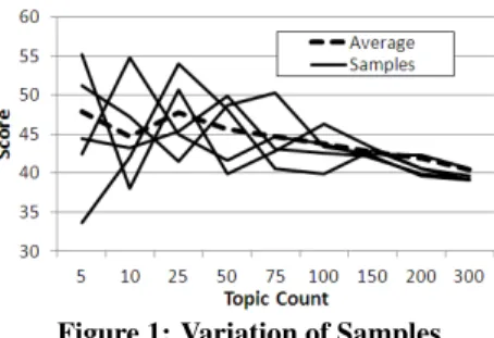
This issue is illustrated in a software context through a replica-tion of work by Grant and Cordy [3] in which they search for the idealtopic count, one of the tuning parameters. Figure 1 shows five observations (the five solid lines) and the average of 48 samples (the bold dashed line) where the highest score indicates the desired topic count. Based on any single observation (any solid line) the analysis concludes that the best topic count is 5, 10, 25, 50, or 75. From the average, it is clear that samples in which 75 is the best choice are quite rare (akin to selecting the particularly tall child).
Those familiar with the work of Grant and Cordy may mistak-enly assume that Figure 1 is a replica of their work. However, there is a key difference: the similar figure shown by Grant and Cordy shows a single observation of multiple programs while Figure 1 shows multiple observations of a single program. Figure 1 illus-trates that considering only a single observation is insufficient.
Unfortunately, taking multiple samples is rare when LDA is ap-plied in SE, where most users consider only a single observation as
Figure 1: Variation of Samples
“the answer.” One challenge in aggregating multiple samples is the topic exchangeability problem: “there is no a-priori ordering on the topics that will make the topics identifiable between or even within runs of the algorithm.· · · Therefore, the different samples cannot be averaged at the level of topics.” [11].
The second challenge when applying LDA is the number and complexity of the tuning parameters employed. Providing an in-tuition for these parameters is this paper’s goal. An alternative to such understanding is to automate their setting based on some external oracle. For example, Panichella et al. [9] use clustering metrics as an oracle and a genetic algorithm to identify settings that lead to good clustering (high metric values). This approach relieves an engineer of the burden of setting the parameters and improves performance for applications where clustering is an ap-propriate oracle. In contrast, the goal of this paper is to provide an understanding of the tuning parameters’ influence and thus to enable their informed setting, which improves the understanding of engineers using LDA and those using LDA-based tools across a wide range of problems. Even those using automatic settings (such as provided by Panichella et al.) will benefit from a better under-standing of the LDA parameters chosen by the automatic technique and their implication.
The tuning parameters can be divided into two groups: LDA parameters and Gibbs sampling settings. The LDA hyper-parameters are features of the model proper, while the Gibbs sam-pling settings are features of the inference method, used to fit the model. In other words, if a different method is selected, such as Variational Inference, only the LDA hyper-parameters would still be relevant. Hyper-parameters are so named because they are the input to the process whose output is two matrices, which are in turn the input parameters used by the generative LDA process to predict document words. The LDA hyper-parametersα,β, andtc, as well as Gibbs sampling settingsb,n, andsiare defined as follows [10]: • α– a Dirichlet prior on the per-document topic distribution • β– a Dirichlet prior on the per-topic word distribution • tc– the topic count (number of topics) in the model • b– the number of burn-in iterations
• n– the number of samples (random variates) • si– the sampling interval
Without an understanding of the impact of each parameter, it is difficult to correctly interpret an LDA model and, more impor-tantly, evaluate the output of an LDA-using tool. It is possible to gain the necessary insight by studying the underlying mathemat-ics [11, 2]; however, this is intensive work. Visualization provides an effective alternative for illustrating the impact of the parame-ters. Fortunately, some parameter’s impact is straightforward. To better understand the tuning parameters five research questions are considered; for each of the five tuning parameterspexcludingsi, the research question “How doespvisually impact LDA output?” is considered. Unfortunately,si, the sampling interval, cannot be adequately studied using current tools (see Section 3.5).
After describing LDA and the six tuning parameters in more de-tail in Section 2, Section 3 considers their impact on production
source code and a controlled vocabulary that makes patterns more evident and easier to describe. Finally, Section 4 takes a further look at the topic count including a replication of the Grant and Cordy study. This replication also hints at future work by consid-ering an implicit parameter, the input corpus. After the empirical results, Section 5 considers related work, and Sections 6 and 7 pro-vide directions for future work and a summary.
2.
BACKGROUND
This section provides technical depth behind LDA, a generative model that describes how documents may be generated. Readers familiar with LDA should skim this section to acquaint themselves with the notation and terminology being used, especially regarding the hyper parametersαandβ.
LDA associates documents with a distribution of topics where each topic is a distribution of words. Using an LDA model, the next word is generated by first selecting a random topic from the set of topicsT, then choosing a random word from that topic’s distribution over the vocabularyW. Mathematically, letθtdbe the
probability of topictfor documentdand letφtwbe the probability
of wordw in topict. The probability of generating wordwin documentd,p(w|d), isP
t∈Tθtdφtw.
Fitting an LDA model to a corpus of documents means inferring the hidden variablesφandθ. Given values for the Gibbs’ settings (b,n,si), the LDA hyper-parameters (α,β, andtc), and a word-by-document input matrix,M, a Gibbs sampler producesnrandom observations from the inferred posterior distribution ofθandφ.
To elucidate the roles of the various Gibbs settings and LDA hyper-parameters, this section describes the effect of each when the others are held constant. The roles ofbandnare straightfor-ward. Gibbs sampling works by generating two sequences of ran-dom variables,(θ(1), θ(2), . . .)and(φ(1), φ(2), . . .), whose
limiting distribution is the desired posterior distribution. In other words, the Gibbs sequences produceθ’s andφ’s from the desired distribution, but only after a large number of iterations. For this reason it is necessary to discard (or burn) the initial observations. The setting
bspecifies how many iterations are discarded. Ifbis too low, then the Gibbs sampler will not have converged and the samples will be polluted by observations from an incorrect distribution.
The Gibbs settingndetermines how many observations from the two Gibbs sequences are kept. Just as one flip of a coin is not enough to verify the probability that a weighted coin lands heads, the Gibbs sampler requires a sufficiently large number of samples,
n, to provide an accurate picture of the topic space. Ifn is too small, the picture is incomplete. In particular, it is inappropriate to take a single observation (n = 1) as “the answer.” Any single observation is next-to-useless on its own.
The third Gibbs setting,si, controls how the resulting samples arethinned. A Gibbs sampler may be afflicted by autocorrelation, which is correlation between successive observations. In this case, two successive observations provide less information about the un-derlying distribution than independent observations. Fortunately, the strength of the autocorrelation dies away as the number of it-erations increases. For example, the correlation between the100th
and103rdvalues is weaker than the correlation between the100th
and102ndvalues. The settingsispecifies how many iterations the Gibbs sampler runs before returning the next useful observation. Ifsiis large enough, the observations are practically independent. However, too small a value risks unwanted correlation. To sum-marize the effect ofb, n, andsi: if any of these settings are too low, then the Gibbs sampler will produce inaccurate or inadequate information; if any of the these settings are too high, then the only penalty is wasted computational effort.
Unfortunately, as described in Section 6, support for extracting interval-separated observations is limited in existing LDA tools. For example, Mallet [7] provides this capability but appears to suf-fer from a local maxima problem1. On the other hand, the LDA im-plementation inR, which is used to produce most of the presented data, does not support extracting samples at intervals. It does com-pute, under the option “document_expects” the aggregate sum of eachθ but, interestingly, notφ, from each post burn-in iteration. However, this mode simply sums topic counts from adjacent itera-tions, which is problematic for two reasons. First, it does not take into account topic exchangeability [11] where a given column in the matrix need not represent the same topic during all iterations. Second, it does not provide access to models other than the final model; thus, there is no support for extracting samples at intervals. An alternate approach, used in this paper, is to run the Gibbs samplernindependent times, recording the last observation of each run. This approach currently has broader tool support and guaran-tees independent observations, though it does require more cycles than sampling at intervals.
Turning to the LDA hyper-parameters, the value ofαdetermines strength of prior belief that each document is a uniform mixture of thetcavailable topics. Thus, it influences the distribution of topics for each document. Mathematically,αcan be interpreted as a prior observation count for the number of times a word from topict oc-curs in a document, before having observed any actual data. When
αis large, the prior counts drown out the empirical information in the data. As a result, the posterior distribution will resemble the prior distribution: a uniform mixture of alltctopics. Conversely, if
αis small, then the posterior distribution will attribute most of the probability to relatively few topics. In summary whenαis large, nearly every document will be composed of every topic in signifi-cant amounts. In contrast whenαis small, each document will be composed of only a few topics in significant amounts.
In a similar way, the role ofβinfluences the word distribution within each topic. A high value forβleads to a more uniform distribution of words per topic. Said another way, larger values of
βfavor a greater number of words per topic, while smaller values ofβfavor fewer words per topic.
Finally, the impact of the number of topicstcis more challeng-ing to characterize but is important as it affects the interpretation of results [11]. Too few topics result in excessively broad topics that include “too much.” That is, topics will tend to capture some com-bination of multiple concepts. On the other hand, too many topics leads to diluted meaningless topics where a single concept is spread over multiple topics. These topics can become uninterpretable as they pick out idiosyncratic word combinations [11].
3.
UNDERSTANDING LDA’S TUNING
Of the tuning parameters described in Section 2 gaining an ap-preciation for the impact ofαandβis key. The central challenge here is to distinguish between topics that concentrate the major-ity of probabilmajor-ity on a single word (or document) from topics that are more uniformly distributed across the entire vocabulary (within the documents). Mathematically, this distinction is captured by the Shannon Entropy of the probabilities in the LDA model. The en-tropy of a probability distribution measures the amount of random-ness. It is defined as the expected number of bits needed to express a random observation from the distribution.
Entropy is maximized when the distribution is uniform and min-imized as probability is concentrated on only a few points. Inφ, the entropyHtof a topictis
1An illustration can be found at www.cs.loyola.edu/~binkley/
topic_models/additional-images/mallet-fixation
Table 1: Programs studied
Size Vocabulary Program Functions (LoC) Size
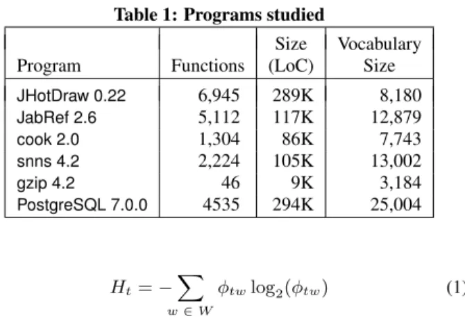
JHotDraw 0.22 6,945 289K 8,180 JabRef 2.6 5,112 117K 12,879 cook 2.0 1,304 86K 7,743 snns 4.2 2,224 105K 13,002 gzip 4.2 46 9K 3,184 PostgreSQL 7.0.0 4535 294K 25,004 Ht=− X w∈W φtwlog2(φtw) (1)
whereWis the set of vocabulary words. The entropy of the topics inθhas the corresponding definition. When the topic distribution is uniform, the entropy reaches its maximum value oflog2(|W|).
Thus, there is no way to predict the next word since any choice is equally likely. When the topic is concentrated on a few dominant words, one has a strong idea of which word will be next for a given topic. As a result, the entropy is small. In the extreme case, if
φtw = 1for wordw, then the next word is no longer random,
and the entropy is zero. To summarize, the entropy of a topic inφ
indicates how many high probability words it contains.
To examine the effect ofαandβon the topic distributions, the average entropy over all topics across the entire sample ofφs is used. Likewise, the average entropy for all documents across the entire sample ofθs is used to understand the effect ofαandβon
θ, where (as withφ) large entropy indicates an emphasis on more uniform distributions. Henceforth, “entropy in φ” refers to “the average entropy of all topics in a sample ofφs” and “entropy inθ” refers to “the average entropy of all documents in a sample ofθs.”
When looking at the entropy inφ, a higher value indicates a more uniform distribution, which is demonstrated by having many im-portant words per topic. Asβincreases, the entropy approaches
log2(|W|), where the uniform prior drowns out the observed data.
With small values ofβ, lower entropy accompanies a non-uniform distribution, which means fewer high-probability words are in each topic. Thus, entropy is expected to increase asβincreases.
Considering the entropy of source code requires some source code. The code used in the empirical investigations, shown in Ta-ble 1, was chosen to facilitate its future comparison with related work [13, 3]. When analyzing source code, thedocumentsused in the LDA model are typically the functions, methods, files, or classes of the source code. In this studyCfunctions andJava meth-ods are used as the documents.
Figure 2 shows the two entropy graphs for the programcook, which are representative of the graphs for the programs in Table 1. In the top plot, the non-bold lines show the average entropy in the observed topic-word distributions across the entire Gibbs sample ofφs plotted against the value ofβon a log-scale. Each non-bold line shows a differentαvalue, with the largest value at the bottom and the smallest value at the top. The bold line shows the average entropy across all values ofα. Similarly, the bottom plot shows the average entropy in the document-topic distribution againstα, where the bold line combines all choices ofβfor a particular choice inα. Each non-bold line shows a differentβvalue, with the largest value at the bottom and the smallest value at the top.
The lines of both graphs have similar shapes, although the lower ones are smoother because more values ofαare considered. The biggest difference between the patterns in the graphs is that the entropy forθexhibits a ceiling effect that is not seen in the graph
Figure 2: Entropy ofφandθfor the programcook(shown
us-ing a log scale forβandαon thex-axis of the upper and lower
graph, and using a linear scale for entropy on they-axis). Each
non-bold line represents a fixed value for the parameter not
represented by thex-axis where the bold line is the average.
forφ. In fact, both curves are S-shaped, but the top part of the S is outside the range of the graph forφ. This is because the maximum entropy for a document (inθ) islog2(tc), but the maximum entropy for a topic (inφ) islog2(|W|). In general, the number of words is much larger than the number of topics, so that the ceiling for the
φgraph is much higher. When suitably large values ofβare used, the entropy ofφwould eventually reach its ceiling.
Starting with the upper graph forφ, asβgrows larger, the en-tropy goes from low (topics of a less uniform distribution domi-nated by a few words) to high (topics of a more uniform distribu-tion more likely to generate a wider range of words). Notice that
β, which directly influences the prior distribution ofφ, has a larger effect thanαon the entropy inφ, as are shown in the top graph of Figure 2. Each line in this graph shows the effect ofβfor a fixed value ofα. Asβranges from10−7to100, the entropy increases from the 3 to 5 range to a maximum around 11. The effect ofα
for a fixed value ofβis seen by observing the width of the band of lines for a particular position on thex-axis. The widest range is only about 0.5 (from 2.5 to 3), which corresponds to the biggest effectαexhibits. From this analysis, it is clear thatβhas a much larger impact on the entropy ofφ.
Turning toθ, the opposite hyper-parameter has the dominant ef-fect. Entropy increases dramatically asαincreases, while the im-pact ofβis small and diminishes asαincreases. Thus, asα in-creases, documents tend to include more topics, which corresponds
Figure 3: Entropy ofφandθfor the controlled vocabulary.
to higher entropy. This pattern is repeated for all values ofβ. Thus, forθ, higher values ofαbring all documents closer to containing all topics. To illustrate the value of understanding these settings, consider a software engineer tasked with refactoring some code us-ing an LDA-based tool where each topic captures a concept from the code. In this case the engineer should choose a smaller value forα; thus causing documents (functions) to receive a dominant topic and consequently suggesting a refactoring.
Figure 2 also shows the interesting interaction betweenαandβ. The hyper-parameterαhas a much bigger impact onφwhen the value ofβis smaller. Conversely,βhas a much bigger impact onθ
whenαis small. Reasons for this are discussed in Section 3.6.
3.1
Control Vocabulary Experiment
Following the advice of Steyvers and Griffiths, a deeper under-standing of the hyper-parameters is illustrated by “generating arti-ficial data from a known topic model and applying the algorithm to check whether it is able to infer the original generative struc-ture" [11]. The rest of this section uses a small fixed vocabulary to study in greater detail the impact ofn, b,si,tc, α, andβon the distributions inθandφ. Figure 3 shows the entropy graphs for the controlled vocabulary. The key observation is that the graphs show the exact same trend as seen in Figure 2. Hence, the intuition gained from the controlled vocabulary can be transferred to models for source code. The slight variation in the shape of the curves of Figure 3 results from the small size of the controlled vocabulary.
Document Name Contents Doc 1 A aa aa aa aa
Doc 2 B bb bb bb bb bb
Doc 3 AB aa aa aa bb bb bb
Doc 4 AC aa aa aa aa cc cc
Figure 4: Vocabulary for the controlled vocabulary experi-ment.
n= 1 n= 1 n= 5 n= 5
Sample 1 Sample 2 Sample 1 Sample 2
Figure 5: The need for multiple samples
The fixed vocabulary, shown in Figure 4, includes three words
aa, bb, and ccorganized in four documents (A, B,AB, and AC) whose names reflect their contents (e.g., DocumentAcontains only wordaa). To better understand the influence ofαandβ, it is nec-essary to first consider the Gibbs settings. While important, their impact is more straightforward. The example was designed so that when usingtc= 3, a topic could be dedicated to each word.
3.2
Sampling Study
It is important to emphasize that the goal of this study is not to determine the “correct” value forn, the number of observations, but rather to illustrate its impact. When considering the impact of
n, fixed values forα,β,b,si, andtcare used. The specific values were chosen to illustrate various patterns. Other choices show the same patterns, although sometimes not as pronounced.
One of the most common errors made when applying LDA in SE is to setn = 1, taking a singleobservationas the topic distribu-tion. The Gibbs sampling process is doing exactly what its name implies,sampling. Thus, asampleof observations isrequiredto gain an understanding of the posterior distribution. To illustrate, Figure 5 shows four charts that all use excessively small values ofn. In all four charts, they-axis shows the sample count where more common samples have larger counts. Thex-axis shows pos-sible outcomes forφ(the same pattern occurs withθ). Thex-axis is shown unlabeled since particular values are unimportant.
The left two charts show samples containing a single observation (n= 1), and the right two charts show samples containing five ob-servations (n= 5). From these four charts several conclusions can be drawn. First, using only one observation givestwo completely different answers: the bars in the left two graphs are in different columns (i.e., different topic models.) Second, while there is some overlap withn = 5, it is not evident that the two charts are sam-ples from the same distribution. For example, the tallest bar in each of then = 5charts is in a different column. The important con-clusion is that whennis too small, an insufficient picture of the distribution is attained. Thus choosing too small a value fornleads to potentially misleading (effectively random) results.
While the goal of this paper is to understand the impact of the parameters, rather than establish appropriate values for them, it is clear from the data that too small a value ofnleads to an incomplete picture. One method to make sure thatnis sufficiently large is to compare several independent samples of sizen. If the downstream results of the analysis are suitably consistent, then one knows that the samples are large enough. At this point, one final sample should be generated using the determined sample size. (The reason for drawing one more sample is that it is statistically inappropriate to use observations both for validating settings and for inference.) As
Table 2: JHotdraw’s color gradient topic across multiple sam-ples
Topic
Number Top 15 Words
22 color gradient space index compon rgb model system min pixel math max red paint arrai 7 color gradient space index model rgb pixel src
paint data param arrai alpha awt focu 34 color gradient space index compon rgb model
system min pixel paint red math max focu
a conservative choice, the charts generated in the remainder of the paper use a minimum value of1000forn, which is likely excessive.
3.3
Canonical Labels for LDA Topics
Before considering the impact of the next parameter, the burn-in
b, a heat-map visualization of the data is introduced. One chal-lenge in aggregating, let alone graphing topic models, is that there is no a-priori ordering of the topics that makes them identifiable between samples. As Steyvers and Griffiths observe, one cannot simply match the topic id numbers over different samples [11]. An illustration of thetopic exchangeability problemis seen in the topic evolution work of Thomas et al. [13]. A replication of their work (shown in Table 2) tracks the topic containing the wordscolor gra-dient. This data shows that this topic is assigned varying topic num-bers across different observations.
Fortunately, for the controlled vocabulary, it is possible to estab-lish topic identity using dominant words and dominant documents. For the topic-word distributionφ, topics are labeled by their high-probability words. High high-probability is established using a cut-off value. For example, consider a topic with the three words “goalie”, “ball”, and “player” that are assigned the probabilities 0.50, 0.45, 0.05, respectively. Using the cut-of of 0.10 for “high probability,” this topic is namedball-goalie. To provide a canonical name, the words of the name are sorted alphabetically. In subsequent obser-vations, any topic that has only probabilities for “goalie” and “ball” greater than the cut-of will be given the same name. These names lead to identifiable topics across observations.
Extending this notion, a set of topicsφcan be represented by a collection of names. Since the topics have no prescribed order, a canonical order is produced by sorting the names of each topic. Thus the topics of a particular observation φare described by a sorted list of (sorted) topic names. For example, the tall bar in the center of the rightmost chart shown in Figure 5 has the name “aa-bb-cc aa bb,” which represents three topics namedaa-bb-cc,
aa, andbb, respectively. This naming scheme makes it possible to visualize the topic-word distribution by counting how often each name-list occurs in thenobservations.
A similar approach is used for the topic-document distribution,
θ, where a topic is named using documents for which it is assigned high probability. This may initially seem backwards, as it is more common to speak of which topics make up a document. However, the documents are fixed while the topic ids suffer from the topic ex-changeability problem. Thus, a topic inθis named using the sorted list of those documents that place a “high” probability on that topic. For example, suppose Documents 1-4 assign probabilities of0.44,
0.55,0.05, and0.24to a topic. Using a cut-off of0.10, this topic would be namedA-B-ACby combining the names of Documents 1, 2, and 4. Similar toφ,θis labeled by a sorted list of topic names.
As shown in Figure 5, a sample of observations can be visualized using a bar chart where thex-axis shows topic names (either lists
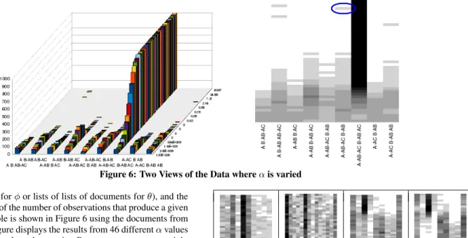
Figure 6: Two Views of the Data whereαis varied
of lists of words forφor lists of lists of documents forθ), and the
y-axis is a count of the number of observations that produce a given name. An example is shown in Figure 6 using the documents from Figure 4. This figure displays the results from 46 differentαvalues which are displayed on thez-axis. Becauseαranges over eight orders of magnitude the non-linear power series10−6∗(9/4)zfor z = 0to45is used. Each sample was produced fromn = 1000
observations. In total, the 3D chart shown in Figure 6 summarizes 46,000 observations. For clarity, topic models observed less than 1% of the time are not shown, which is fewer than 460 samples.
The chart clearly shows that choosing different values forαhas a dramatic influence on the topic models. Using larger values of
α, the dominant name list isA-AB-AC B-AB AC, corresponding to three topics: a topic dominant in the three documentsA,AB, andAC
(capturing the wordaa), a topic dominant toBandAB(capturing the wordbb), and a topic dominant toAC(capturing the wordcc). This validates using controlled vocabulary as suggested Steyvers and Griffiths [11].
The same patterns can be seen using heat maps where gray scale replaces thez-axis (e.g., as seen in the right of Figure 6). Although the 3D view better highlights contour differences, it can obscure values hidden behind tall bars. For example, the encircled light grey bar to the left of the top of the black bar in the heatmap of Figure 6 is hidden in the 3D chart of the same data. Heatmaps are used in the remainder of the data presentation.
3.4
Burn-In
When considering the burn-in intervalb, the following values are used:n= 1000,tc= 3,si=∞(see Section 3.5), andβ= 10−2, (these values aid in the presentation as they produce sufficiently interesting structure). Other values show the same pattern, although less pronounced.
The Gibbs sampling process starts by assigning each topic a probability of1/tcunder each document, and each of the words in the input corpus a probability of1/|W|under each topic where
W is the set of unique words in the corpus; thus, the early sam-ples are not useful as too much of this initial uniform assignment remains. Forφ, the heat map for this initial assignment appears as a single black line with the name listaa-bb-cc aa-bb-cc aa-bb-cc. The initial value forθalso produces a single black line.
The burn-in study considers values ofbranging from 1 to 65,536 in powers of two. A subset of these are shown in Figure 7.2 As is evident in the chart forb= 1, after a single iteration the initial con-2The remaining graphs can be found at www.cs.loyola.edu/~binkley/
topic_models/additional-images/burn-in-study.
1 2 32 2048
Figure 7:φBurn-in Study (θshows the same pattern)
figuration (the single black line) is still dominant. However, there are also nine other columns in the graph indicating some influences from the data. Early on this variation increases with more possibil-ities appearing on thex-axis (more columns). By iteration 32 the final distribution is becoming evident (e.g., there are fewer columns in this graph than the one for 2 iterations). This is because some of the topics fall below the 1% threshold. By iteration 2048 the distributionofφhas stabilized and remains unchanged through the rest of the 65,536 iterations. This experiment was replicated sev-eral times. While there are minor variations in the early iterations, the same general pattern emerged: a differing initial explosion and then arrival at the same final distribution.
Based on this data subsequent experiments were designed to have a minimum burn in ofb= 2000. A smaller value is likely accept-able; thus makingb= 2000a conservative choice. (As noted in Section 3.5, the effective burn in turned out to beb= 22,000.)
3.5
Sampling Interval
The final Gibbs setting is the sampling interval,si. Given an implementation capable of correctly extracting multiple variates, the algorithm would iteratebtimes and then start sampling, tak-ingn samples at intervals ofsi. These samples would be taken at iterationsb+si, b+ 2∗si, ,· · ·b+n∗si. However, because sampling proved problematic with three LDA tools available (see Section 6), samples were collected by constructingnseparate mod-els, using the final iteration as the observation (the random variate). This leaves the empirical study ofsito future work after tools bet-ter support sampling. Because the original design called for each execution to yieldn= 1000samples with a sample interval up to
si= 20, each execution generates one data point with an effective burn-in ofb= 22,000.
3.6
Impact of
αand
βThis section considers the impacts first ofβ, then ofα. The other parameters are fixed withb= 22,000,n= 1000, andtc= 3. The initial discussion focuses on the length and frequency of the name lists that label thex-axis of the heat maps forφ(top row) andθ
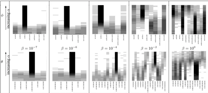
6 increasing α φ β= 10−7 β= 10−6 β= 10−4 β= 10−2 β= 100 6 increasing α θ
Figure 8: Impact ofαandβ(Top:φ; Bottom:θ)
(bottom row) of Figure 8. They-axis on each heat map showsα, which is the non-linear power series,10−6∗(9/4)zforz= 0to45. Each vertical pair of heat maps (those in the same column) show a given value ofβ.
To begin with, a smaller value ofβfavors fewer words per topic. In the top row of Figure 8, the heat maps concentrate onφ={aa bb cc}, for which each topic is dominated by a single word. For very low values ofβ, only seven distinct name lists appear (re-call that the heat maps are filtered to only show word-topic matri-ces that represent at least1%of the observations). Three of these consist solely of single word topics. In the remaining four, only a single topic shows multiple words. Values ofφcontaining more than one multi-word topic do not appear untilβ = 10−4. Asβ
increases, multi-word topics appear more commonly. Atβ= 102
(not shown), each value ofφcontains at least one multi-word topic. Another way of expressing the impact of highβ is that it en-courages greater uniformity (i.e., greater influence from the prior). Greater uniformity leads to topics that include multiple significant words. This pattern is evident in theβ= 100
heat map by the exis-tence of very long topic names. In this heat map, the second column from the right has the name listaa-bb-cc aa-bb aa-cc, which is two names shy of the maximumaa-bb-cc aa-bb-cc aa-bb-cc.
Similar patterns are evident in the topic-document heat maps (bottom row of Figure 8). In this case, topics with more domi-nant words can be combined in a greater number of ways. As an extreme example, suppose that the topics aret1=aa,t2=bb, and
t3=cc. Since Document 3 contains bothaaandbb, it will almost
certainly place significant weight on topicst1andt2. On the other
hand, if every topic has a high probability of each word (i.e., aa-bb-cc), it is possible for Document 3 to consist of only a single topic. Thus, the number of entries on thex-axis increases asβincreases, because each topic is potentially relevant to more documents. The lesson here is that, whileβdirectly controls the prior forφandα
directly controls the prior forθ, both tuning parameters influence both matrices due to the dependence between the per-topic word distributions and the per-document topic distributions.
Turning toα, whenαis small the LDA model emphasizes fewer topics per document. This creates pressure to have complex topics or, in other words, topics with multiple words that can individu-ally generate the words of a given document. Conversely, asα
increases the LDA model moves toward encouraging more topics per document. This enables (but does not require) simpler topics with a smaller number of dominant words. These patterns are clear in the upperβ=10−2heat map forφ. For example, the longest name list,aa-bb-cc aa-bb aa-cc, labels the7thcolumn while one of the shortest aa bb cc, labels the3rd
column. From the heat map, models that include the long name list are more common at the bottom of the heat map whereαis small and grow less com-mon (a lighter shade of gray) asαincreases. In contrast, column three grows darker (more models have these topics) asαincreases. This pattern is quite striking with smaller values ofβ. In particular, whenβ= 10−7
andαis large, the only value ofφthat appears is
aa bb cc. A software engineer using an LDA-based tool to, for ex-ample, summarize methods might prefer this setting as each topic is dominated by a small number of key words.
In the topic-document heat map (θ, bottom) forβ = 10−2, the
pressure toward multiple-topic documents whenαis large is evi-dent in the column with the black top. This column captures models with the name listA-AB-AC,B-AB, andACwhere two of the topics have multiple significant documents. These topics have the single significant wordsaa,bb, andcc, respectively. The fourth column from the right has the name listA-AC B AB. This list is the most frequent of the short name lists and is clearly more common where
αis small because the pressure to have fewer (but more complex) topics for each document leads to topics being significant to fewer documents (i.e., yielding shorter topic name lists).
The heatmaps provide an intuition for the parameters, but are only effective for the controlled vocabulary. They do not scale well to larger data sets. For example, even the smallest vocabulary ofgzipincludes 3,184 unique words, resulting in23184tc possible names forφ. Recall that the motivation behind the topic names was to identify patterns in the dominant words of the topics ofφand the dominant documents for a given topic ofθ. Fortunately, this distinction is also captured in the Shannon Entropy of the probabil-ities in the LDA model. For example, topics with long names have many high probability words and therefore a larger Shannon En-tropy, but topics with short names have few high probability words and a smaller Shannon Entropy.
The entropy graphs for the controlled vocabulary, shown in Fig-ure 3 mirror the patterns seen in the heat maps. For example, in the
upper graph forφ, asβgrows larger, the entropy goes from low (short topic names corresponding to a less uniform distribution) to high (more multi-word topic names). As expectedβ, which di-rectly specifies the prior distribution ofφ, has a larger effect thanα
on the entropy inφ. That is, a larger change inφ’s entropy is ob-served when fixingαand varyingβ, than when the reverse is done. This is particularly true for larger values ofβ.
Encouragingly, the same pattern is seen in Figure 8. For exam-ple, in the heat map forφwhenβ = 10−7, more of the observa-tions have longer names (signifying higher entropy) at the bottom whenαis small than at the top whereαis large (where the three topics are each dominated by a single word). Far more dramatic is the increase in topic-name length asβ increases. The preva-lence of observations with the longest names by the timeβ= 100
corresponds to more uncertainty regarding the word chosen for a given topic, which in turn corresponds to higher entropy. Finally, with larger values ofβ, the effect ofαdiminishes. Here the prior drowns out the data and entropy increases to the maximum possible value oflog2(|W|).
Turning toθ, the opposite hyper-parameter has the dominant ef-fect: entropy increases dramatically asαincreases, while the im-pact ofβis small and diminishes asαincreases. This can be seen in the heat map forθwithβ= 10−7in Figure 8 where the longest nameA-AB-AC, B-AB, ACgrows more common (its bar gets darker) asαincreases. Thus asαincreases longer names are more com-mon, which corresponds to higher entropy. This pattern is repeated for all values ofβ. For example, whenβ = 100, the topics with
longer names become more common (their bars get darker) toward the top of the chart whereαis larger. Thus, forθ, higher values ofαbring all documents closer to containing all topics (i.e., long topic names are more common). Whenαis small, documents tend to focus on a few particular topics.
In summary, the variety seen in Figure 8 clearly illustrates that care is needed when choosing values forαandβ. One goal of this paper is to visually provide an intuition for their impact on LDA models (rather than an attempt to establish “best” values). Clearly, the “best” values forαandβare problem- and goal-dependent. For example, when trying to generate concept labels, a smaller value of
βwould lead to topics that included fewer words in the hope of pro-viding more focused concept labels. In contrast, when performing feature location a larger value forαwould encourage more topics per document and thus increase recall as a topic of interest would be more likely to be found in the code units that truly implement the feature. In summary, both the problem being solved and the objectives of the software engineer using the solution impact the choice ofαandβ. This underscores the values of the goal of this paper: to improve engineer and researcher comprehension regard-ing their impact in order to improve their use of LDA models in software engineering.
3.7
Topic Count
The final LDA parameter considered is the topic count. The models considered above with the controlled vocabulary use three topics, which is large enough for each word to have its own topic depending on the influences ofαandβ. This flexibility helps to illustrate the impact ofαandβ.
Steyvers and Griffiths observe that “the choice of the number of topics can affect the interpretability of the results [11].” To sum-marize their conclusions, too few topics results in very broad topics that provide limited discrimination ability. On the other hand, hav-ing too many topics leads to topics that tend to capture idiosyncratic word combinations. They go on to note that one way to determine the number of topics is to “choose the number of topics that leads
to best generalization(sic) performance to new tasks [11].” This is in essence the approach used by Panichella et al. [9] and by Grant and Cordy [3] who tune topic count to a specific task. The next section considers a source-code example.
At one extreme, with a single topic the model degenerates to a unigram model, which posits that all documents are drawn from a single distribution captured byφ. At the other extreme an infinite number of topics is possible because two topics need only differ in the weights they assignment to the words. The controlled vo-cabulary is too small to effectively study the topic count. A more meaningful empirical consideration is given in the next section us-ing production source code.
4.
TOPIC COUNT IN SOFTWARE
To further study the impact of topic count, a replication of a Grant and Cordy experiment is presented. This is followed by a look at topic count’s impact on entropy. Grant and Cordy’s goal is to determine “a general rule for predicting and tuning the ap-propriate topic count for representing a source code” [3]. This is done using heuristics to evaluate the ability of an LDA model to identify related source code elements. In its strictest application, the heuristic considers two functionsrelatedif they are in the same source-code file. This can be relaxed to consider two functions as related if they are in the same directory, have the same parent di-rectory, etc. In this replication,relatedis defined as “in the same directory."
For a given functionf, an LDA model is used to identify the top
N functions related tof. This identification is done using cosine similarity between each function’s topic vector and is described in greater detail by Grant and Cordy [3]. The quality of the LDA model is measured by counting the number of the topNfunctions that are related according to therelatedheuristic. The count ranges from one (a function is always related to itself) toN. The average count over all functions is thescoreassignment to the LDA model. To assess the impact of topic count, Grant and Cordy compare LDA model scores for a range of topic counts, using several pro-grams includingPostgreSQL(http://www.postgresql.org), which is used in this replication. While the degree of sampling in the origi-nal is unclear (unless otherwise noted) each data point in the figures of this section represents the average ofn= 48observations.
In the original experiment, comments were stripped from the source code. To enable consideration of their impact, the repli-cation considers models with and without comments. In addition, it considers the impact of vocabulary normalization on each cor-pus [4]. Normalization separates compound-word identifiers and expands abbreviations and acronyms so that the words from iden-tifiers better match the natural language found elsewhere (such as the requirements or comments).
The resulting scores for each of the four corpora are shown in Figure 9 for bothN = 10andN = 50. The impact of having too-large a topic count is evident, especially withN = 50. Past
tc= 50topics, all four corpora show a steady decline. The impact of too small a topic count is more pronounced in the upper graph, where including comments tends to increase the size of the vocab-ulary. Comparing the solid black line (without comments) and the solid gray line (with comments), early on there are too few topics in the model, which yields lower scores for the larger vocabulary. The lack of discrimination ability is evident in these broad topics. Consistent with Grant and Cordy’s results, these data illustrate the consequences of choosing too few or too many topics.
Finally, normalization’s impact can be seen by comparing corre-sponding solid and dashed lines. For the comment-free corpora (black lines) normalization has little impact. This is in essence
Replication withN= 10(min score = 10, max score =102)
Replication withN= 50(min score = 50, max score =502)
Figure 9: Grant and Cordy Replication
because universally replacing an abbreviation such ascntwith its expansion,count, does not change the word frequencies used to build the LDA model. Rather, it simply swaps one word for an-other. However, when comments are included, they tend to include “full words” and thus replacingcntwithcountbrings the vocab-ulary of the source code more in line with that of the comments. This change does impact the counts used to build the LDA model. In essence there is a reduction and a focusing of the vocabulary leading to a higher score. For example, rather than requiring both
cntandcount, after normalizationcountsuffices.
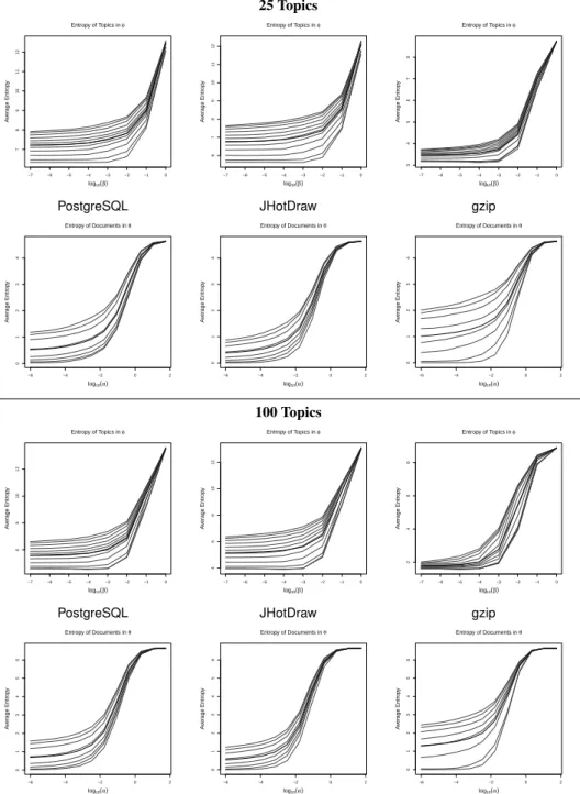
Another way of considering topic count returns to the entropy graphs. Figure 10 shows the entropy graphs for three of the six programs from Table 1 using an LDA model with either 25 or 100 topics. The charts for 50, 200, and 300 topics show the same trends. An additional program,cook, is shown in Figure 2. The graphs for the two remaining programs show the same pattern.
The graphs in Figure 10 show interesting interactions amongtc,
β, andα. Comparing a specific program’s two entropy graphs for
φ, reveals that the higher topic count intensifies the effect ofβ. Notice that they-axis ranges from a lower number whentc= 100
compared totc = 25. Intuitively, when words are split among
tc = 100topics, each topic may concentrate on relatively fewer
words, compared to when there are only25topics. As explained in Section 3, this results in lower entropy fortc= 100, as the topic is more predictable.
Whiletcaffects the minimum observed entropy, it does not change the maximum. For a model with|W|words, the entropy for a topic has an upper limit oflog2(|W|); it is defined by the number of words, but not the number of topics. Whenβis set very high, it pushes each topic toward a uniform distribution of words and the entropy toward the upper limit. Interestingly, the topic count af-fects howquicklythe entropy reaches this limit. In other words,
whentc= 100, the entropy graphs forφstart lower, but approach
the maximum more quickly. For example, looking at the entropy curves forPostgreSQL, thetc= 100graph exhibits a steeper slope in the middle piece of the S-curve, which is where the increase in
entropy is most prominent. As a result, when considering a large value ofβ, the entropy tends to be higher whentc= 100. Specifi-cally, the entropy atβ= 10−1is higher whentc= 100for all three programs in Figure 10. As a minor note, the interaction betweenβ
andtccauses a small quirk in the entropy graphs forgzip. Namely, every entropy curve has a ceiling effect as the entropy approaches its maximum possible value. At some threshold, increasingβorα
cannot have a large effect on the entropy because it is almost maxi-mized already. This results in the prominent S-pattern in the graphs forθ. However, most of the graphs forφdo not show this pattern becauseβdoes not reach the threshold. Essentially, only part of the S-pattern is inside the range of the graph. The ceiling effect only appears forgzipwhentc= 100because the small vocabulary size results in a low ceiling. The large number of topics causes the entropy to approach this ceiling rapidly.
The interaction between topic count andα is straightforward. For a given value ofα, the entropy is larger whentcincreases from
25to100. This is most obvious for large values of α, when the entropy is near its maximum,log2(tc). Thus, the graphs with100
topics have a higher ceiling. Nevertheless, the effect oftcis similar for small values ofα. A more subtle facet of the interaction is that the effect oftcfor large values ofαseems to persist even when taking into account the different maximum values, where the model is closer to the uniform distribution whentcis larger.
5.
RELATED WORK
Two recent studies have considered determining various subsets of the tuning parameters. The first is the work replicated in Sec-tion 4 where Grant and Cordy determine the optimal number of topics for 26 programs [3]. Section 4 considered just one of these. They conclude by noting that “the number of topics used when modeling source code in a latent topic model must be carefully considered.” The impact of topic count on model quality is visu-ally evident in Figure 9. One question Grant and Cordy raise is the value of retaining comments. This question was considered in the replication described in the previous section.
Second, the work of Panichella et al. [9] employs a genetic al-gorithm to identify “good” hyper-parameter values. The challenge here is (automatically) judging “goodness.” They do so by mapping the LDA output to a graph and then applying a clustering algorithm where existing clustering metrics are used as a proxy for “good”. Here the use of clustering drives the LDA models to favor single thought topics because such topics produce more cohesive clusters. The impact on the hyper-parameters is to favorβbeing small and
αbeing large. The approach is validated by showing that it im-proves performance on three software engineering tasks, traceabil-ity link recovery, feature location, and software artifact labeling. In light of the data presented in Section 3, it would be interesting to explore the interplay between the sampling of the posterior distri-bution, which goes un-described, and the genetic algorithm, which searches over multiple models.
6.
FUTURE WORK
Several extensions to this work are possible. As described in Section 2 commonly used implementations of Gibbs sampling pro-vide little support for extracting multiple interval-separated sam-ples. To ensure independence, the data presented in this paper usednindependent observations (nindependent executions of R’s Gibbs sampling process).
The Gibbs’ implementation in Mallet [7] provides an option to output everysithmodel. However, when configured to do so it is quite clear that the samples are correlated even withsiset as high
25 Topics −7 −6 −5 −4 −3 −2 −1 0 7 8 9 10 11 12 Entropy of Topics in φ log10(β) A v er age Entrop y −7 −6 −5 −4 −3 −2 −1 0 6 7 8 9 10 11 12 Entropy of Topics in φ log10(β) A v er age Entrop y −7 −6 −5 −4 −3 −2 −1 0 3 4 5 6 7 8 Entropy of Topics in φ log10(β) A v er age Entrop y
PostgreSQL JHotDraw gzip
−6 −4 −2 0 2 0 1 2 3 4 Entropy of Documents in θ log10(α) A v er age Entrop y −6 −4 −2 0 2 0 1 2 3 4 Entropy of Documents in θ log10(α) A v er age Entrop y −6 −4 −2 0 2 0 1 2 3 4 Entropy of Documents in θ log10(α) A v er age Entrop y 100 Topics −7 −6 −5 −4 −3 −2 −1 0 6 8 10 12 Entropy of Topics in φ log10(β) A v er age Entrop y −7 −6 −5 −4 −3 −2 −1 0 4 6 8 10 12 Entropy of Topics in φ log10(β) A v er age Entrop y −7 −6 −5 −4 −3 −2 −1 0 2 4 6 8 Entropy of Topics in φ log10(β) A v er age Entrop y
PostgreSQL JHotDraw gzip
−6 −4 −2 0 2 0 1 2 3 4 5 6 Entropy of Documents in θ log10(α) A v er age Entrop y −6 −4 −2 0 2 0 1 2 3 4 5 6 Entropy of Documents in θ log10(α) A v er age Entrop y −6 −4 −2 0 2 0 1 2 3 4 5 6 Entropy of Documents in θ log10(α) A v er age Entrop y
Figure 10: Entropy ofφandθfor the programsPostgreSQL,JHotDraw, andgzip.
as 997. The degree of auto-correlation is related toβ. An empirical investigation indicates that Mallet gets “stuck” in different local maxima. Separate executions of the tool successfully sample the posterior distribution, but further investigation is warranted.
Finally, the last study considered four variations of the input cor-pus, and thus the future work concludes by considering the way in which the source code is mapped into an LDA input corpus. There are a range of other preprocessing options possible such as stem-ming and stopping.
7.
SUMMARY
This paper aims to improve the understanding of the LDA mod-els used by software engineers by raising their awareness of the effects of LDA tuning parameters. The empirical study visually
il-lustrates the impact of these parameters on the generated models. The better understanding of LDA made possible through visualiza-tion should help researchers consider how best to apply LDA in their work. In particular, sampling must play a bigger role in the discussion of tools that depend on LDA models. Such discussion should include how samples are aggregated since this is dependent on the task at hand.
8.
ACKNOWLEDGEMENTS
Support for this work was provided by NSF grant CCF 0916081. Thanks to Malcom Gethers for his advice working with LDA and R, Scott Grant for his assistance in the replication of the topic count study, and Steve Thomas and Jeffrey Matthias for their assistance in the replication of the topic evolution work.
9.
REFERENCES
[1] H. Asuncion, A. Asuncion, and R. Taylor. Software traceability with topic modeling. InProceedings of the 32nd ACM/IEEE International Conference on Software
Engineering-Volume 1, pages 95–104. ACM, 2010. [2] D. Blei, A. Ng, and M. Jordan. Latent dirichlet allocation.
Journal of Machine Learning Research, 3, 2003. [3] S. Grant, J. Cordy, and D. Skillicorn. Using heuristics to
estimate an appropriate number of latent topics in source code analysis.Science of Computer Programming, http://dx.doi.org/10.1016/j.scico.2013.03.015, 4 2013. [4] D. Lawrie and D. Binkley. Expanding identifiers to
normalizing source code vocabulary. InICSM ’11: Proceedings of the 27th IEEE International Conference on Software Maintenance, 2011.
[5] Erik Linstead, Paul Rigor, Sushil Bajracharya, Cristina Lopes, and Pierre Baldi. Mining concepts from code with probabilistic topic models. InProceedings of the twenty-second IEEE/ACM international conference on Automated software engineering, pages 461–464. ACM, 2007.
[6] Stacy K Lukins, Nicholas A Kraft, and Letha H Etzkorn. Source code retrieval for bug localization using latent dirichlet allocation. InReverse Engineering, 2008. WCRE’08. 15th Working Conference on, pages 155–164. IEEE, 2008.
[7] A. McCallum. Mallet: A machine learning for language toolkit, 2002.
[8] R. Oliveto, M. Gethers, D. Poshyvanyk, and A. De Lucia. On the equivalence of information retrieval methods for
automated traceability link recovery. InProgram Comprehension (ICPC), 2010 IEEE 18th International Conference on, pages 68–71, 2010.
[9] A. Panichella, B. Dit, R. Oliveto, M. Di Penta,
D. Poshynanyk, and A. De Lucia. How to effectively use topic models for software engineering tasks? an approach based on genetic algorithms. InACM/IEEE International Conference on Software Engineering (ICSE’13), May 2013. [10] I. Porteous, D. Newman, A. Ihler, A. Asuncion, P. Smyth,
and M. Welling. Fast collapsed gibbs sampling for latent dirichlet allocation.14th ACM SIGKDD international conference on Knowledge discovery and data mining, 3, 2008.
[11] M. Steyvers and T. Griffiths.Probabilistic Topic Models in Latent Semantic Analysis: A Road to Meaning, Landauer, T. and Mc Namara, D. and Dennis, S. and Kintsch, W., eds. Lawrence Erlbaum, 2007.
[12] Stephen W Thomas. Mining software repositories using topic models. InSoftware Engineering (ICSE), 2011 33rd International Conference on, pages 1138–1139. IEEE, 2011. [13] Stephen W. Thomas, Bram Adams, Ahmed E. Hassan, and
Dorothea Blostein. Modeling the evolution of topics in source code histories. InProceedings of the 8th Working Conference on Mining Software Repositories, MSR ’11, 2011.
[14] Kai Tian, Meghan Revelle, and Denys Poshyvanyk. Using latent dirichlet allocation for automatic categorization of software. InMining Software Repositories, 2009. MSR’09. 6th IEEE International Working Conference on, pages 163–166. IEEE, 2009.