Some Effects of Transaction Taxes Under Different Microstructures

Q

F

R

C

Research Paper 212 December 2007

Some effects of transaction taxes under

different microstructures

Paolo Pelizzari and Frank Westerhoff

DIFFERENT MICROSTRUCTURES

PELLIZZARI PAOLO AND WESTERHOFF FRANK

Abstract. We show that the effectiveness of transaction taxes

depends on the market microstructure. Within our model, hetero-geneous traders use a blend of technical and fundamental trading strategies to determine their orders. In addition, they may turn inactive if the profitability of trading decreases. We find that in a continuous double auction market the imposition of a transaction tax is not likely to stabilize financial markets since a reduction in market liquidity amplifies the average price impact of a given order. In a dealership market, however, abundant liquidity is provided by specialists and thus a transaction tax may reduce volatility by crowding out speculative orders.

1. Introduction

As, for instance, illustrated by [27], financial markets are quite volatile and may display severe bubbles and crashes. Since asset prices are de-termined by the orders of market participants, one may argue that speculative activity is at least at some times excessive in financial mar-kets. Keynes [15] and Tobin [32] therefore suggested to introduce a Transaction Tax (TT) in financial markets in order to curb specula-tive activity. Their basic argument rests on the assumption that there are two types of market participants: stabilizing long-term investors and destabilizing short-term speculators. A small transaction tax has presumably no impact on long-term investors so that their stabilizing influence on the market should remain intact. However, even a modest transaction tax may have a strong impact on the profitability of short-term speculators. Keynes and Tobin suspect that this trader type is the main trigger for the recurrent turbulent behaviour of financial mar-kets. If destabilizing short-term speculative orders decrease, financial markets should become more efficient.

The optimistic view of Keynes and Tobin has been supported by a number of prominent economists, including [29], [30], or [8]. For a general discussion of this topic see [26], [33] and [28]. But there are

Key words and phrases. Transaction tax, Tobin tax, microstructures, agent-based models, liquidity.

Part of this work was done while the first author was at the Quantitative Finance Research Center (QFRC, University of Technology Sydney), whose financial sup-port is gratefully acknowledged.

also opponents to this proposal. For instance, a few empirical papers conclude that transaction taxes may not contribute to a stabilization of financial markets ([34], [14], [1], [12]). However, one should note that these empirical studies face some restrictions. For instance, the paper by Umlauf investigates the case were Sweden introduced a transaction tax rate of 2 percent and today probably nobody recommends such a high transaction tax. Further sceptical comments concerning the empirical research may be found in [35].

Some authors have also tried to address this open research question from an agent-based financial market perspective. According to sur-vey studies (e.g. [31]), market participants rely on both technical and fundamental trading rules to determine their orders. Guided by these observations, models have been developed which explore the impact of heterogeneous interacting agents upon the market dynamics. This ap-proach, recently reviewed in [13], [17] and [21], has proven to be quite successful. For instance, these models are able to replicate some im-portant stylized facts of financial markets such as bubbles and crashes, excess volatility or fat tails for the distribution of returns and thereby add to our understanding of the working of financial markets. Key contributions include [5], [16], [3], [6], [20], [2], [9] or [25].

Given the power of these models, it seems natural to use them as artificial laboratories to test the effectiveness of transaction taxes. An early contribution in this direction is [11]. Frankel develops a simple exchange rate model with two types of agents: Investors believe that the exchange rate will return towards its fundamental value while spec-ulators are convinced that the exchange rate will trace out a bubble path. Frankel analytically shows that an exogenous increase in the frac-tion of investors leads to a reducfrac-tion in the variability of the exchange rate. The opposite is true when the fraction of speculators increases. According to Frankel, a transaction tax could be expected to lower the fraction of speculators or to raise the fraction of investors. Either way, he suspects, the volatility of the exchange rate will decrease.

[36] and [37] develop models in which the agents may endogenously select between technical or fundamental trading rules. In addition, they may be inactive. The agents’ choice process depends on the strategies’ past performance. A strategy that did well in the past will be followed by more agents in the future. These two models predict that the im-position of a small transaction tax is likely to increase market stability since it crowds out speculative activity. Only when the tax rate is set too high, market efficiency may decrease.

[7] and [22] claim that transaction taxes may have a negative impact on market liquidity. This is an important observation since market liquidity is inversely related to the price responsiveness of a given order (see [18], [10], [19]). This means that the lower liquidity, the stronger the price change with respect to a given incoming order. Both papers

find that if this effect is taken into account the stabilizing impact of a transaction tax decreases.

The goal of our paper is to systematically reconcile the apparently contrasting results provided in the aforementioned literature. For this reason, we develop a model along the lines of [4] by Chiarella and Iori (CI) in which agents rely on a blend of technical, fundamental and random trading strategies. However, if past trading generates losses, a trader may also (temporarily) retreat from the market. The price adjustment is modelled both in a continuous double auction and in a dealership environment. Both settings have the potential to gener-ate reasonable price dynamics. So, our model allows comparing the implications of transactions taxes within different institutional market settings.

Our simulation experiments reveal that the consequences of transac-tion taxes depend on the liquidity totally provided. When abundant exogenous liquidity is provided, the tax is stabilizing, but this result does not hold in other settings, as in the presence of market protocols where liquidity is endogenous and fluctuating. Most of the theoretical work, e.g. [37], is indeed based on a market maker scenario in which infinite liquidity is provided. On the other hand, most empirical work collects data from more realistic market structures where liquidity im-perfections are amplified by the tax, resulting in little effect or even in a deterioration of market quality. More subtly, our work suggests that finer details in the functioning of the market might ultimately decide if the introduction of a Tobin tax is stabilizing. Levying a transaction fee is always reducing the volume, this, in turn, is harmful only if liquidity is affected and this triggers an increment in volatility. However, if mar-ket makers offer widely liquidity, the tax is effective and does produce smaller volatility. Surprisingly, the imposition of a transaction tax has in neither market protocol a clear relation to the distortion, i.e. to the average absolute deviation between prices and fundamentals.

The paper is organized as follows. In section 2, we discuss how the market participants determine their orders. Our setup is related to the one presented by CI, yet we assume in addition that the market entry decision of the traders is endogenous and depends on profit considera-tions. In section 3, we introduce the market protocols. Order induced price adjustments take place either within a continuous double auc-tion market or within a dealership market. In secauc-tion 4, we present our results. The last section concludes and two Appendixes provide additional information.

2. _{The model}

We consider a market for one risky asset (stock) and cash. We as-sume that the interest rater = 0 or, equivalently, that the interest rate

whose initial endowments are Si0 and Ci0 units of stock and cash,

re-spectively. The holdings of the agents are updated in the obvious way whenever there is a transaction. They cannot go short or lend/borrow money. There are multiple trading sessions (days) and every agent is selected in random order within a single day.

Agents record their trading performance and accordingly switch at the end of the day to an active or idle state. We denote with Xi(t)∈ {A, I} the state of i-th agent at time t. Inspired by the work of CI, each agent at time t, if active, submit an order to the market based on an estimate of future return

ri_t+1 =g₁ip

f _−p

t pt

+g₂irLi+niit,

where the weights g₁i > 0, g₂i, ni represent the fundamental, chartist

(trend-chasing or contrarian if g2 is positive or negative, respectively)

and random component,it ∼N(0,1) andrLi is the average past return

over a time-span of length Li ∈ {1, . . . , Lmax}. In detail, g₁i ∼ |N(0, σ1)|; g₂i ∼ N(0, σ2); ni ∼ N(0, σn); rLi = 1 Li Li X j=1

logpclose_t−j −logpclose_t−j−1,

where pclose

t is the closing price in session t. The weights g1i, gi2, ni and

the length Li are independently sampled from the respective

distribu-tions only once at the beginning of the simuladistribu-tions and never changed.

Equipped with r_ti₊₁ the agent can compute expected future price as

ˆ

pi

t+1 =ptexp(rti+1).

Agents are hence heterogeneous in their own blending of different forecasting methods and in the extent of past close-to-close returns they take into account. Alternatively, we can interpret their random component as coming from liquidity shocks with no link to any strategic trading behaviour.

We assume that the agents can submit a unique limit order for one unit of the asset per day. A limit order is a couple, quantity-limit price (qτ, lτ) that is submitted in a randomly selected instant τ of a given

day. Assume that t < τ < t+ 1. Each active trader is posting an order

(qiτ, liτ), where

qiτ = sgn(ˆpit+1−p

close

t−1 ),

is depending on the difference between the forecast and the last avail-able closing price and

liτ = ( bpˆi t+1(1−κi)c if qiτ >0; dpˆi t+1(1 +κi)e if qiτ <0,

where κi is an individual aggressiveness parameter, that reduces the

bid when buying and increases the ask when selling. Observe that all limit prices are integers as required by the trading protocols that will be described in the sequel.

The active agents that were able to trade one unit during the day at some price piτ, t < τ < t+ 1 compute their myopic profits

π(i, t) =

(

pclose

t −piτ −tax if i-th agent is a buyer;

piτ −pclose_t −tax if i-th agent is a seller.

Then the same agents (that succeeded in trading) adjust an individual smoothed profit measure as

Ui,t = (1−η)π(i, t) +ηUi,t−1.

Traders can switch strategy with probability µ at the end of each

day, when the closing price becomes available and evaluation of their profits is possible. Agents switch to the active state with individual probability

φi,t =

exp(Ui,t/b)

exp(Ui,t/b) + exp(0) .

Hence the future state of an agent is given by

Xi(t+ 1) =

(

A with probabilityφi,t;

I with probability 1−φi,t.

Observe that switching is based on profitability in both states: Ui,t

denotes the gains in the active state while 0 is obviously the gain in the idle state where no trade can occur. The bigger the gains in the active state, the bigger is the probability to stay (or switch to) active.

Here b > 0 is a parameter related to the intensity of switching: large

b make the agents insensitive to profits and prone to be idle or active

with equal probability. On the contrary, small b will make them more

likely to switch to the most profitable state at time t+ 1.

This model of behaviour is assuming that the imposition of a tax is pushing people to the idle state by shrinking their gains. This is ob-viously an over-simplified mechanism in that agents could, say, incor-porate the tax losses in their forecasts. However, this straightforward mechanism is used a number of relevant works , see [2], and is close to the basic intuition that (too) active agents should move to the idle state being excessive trading penalized by a TT.

2.1. Timing. It is useful to recap in detail how the model is running. A typical trading day (t-th day) develops as follows:

(1) At t− the closing price pclose_t−1 of the previous session, the past returns’ averages rLi and the states of agents are known;

(2) Beginning at time t+_{, agents trade at random times t < τ <}

t+ 1, submitting their orders to the market (with no certainty that they will be executed);

(3) In (t+ 1)− the closing pricepclose

t for day tis known and

active-successful traders hence can compute profits π(i, t) and adjust their performance measure Ui,t. Notice that if an agent is

un-able to trade, his/her π and U are held unchanged. This is

happening for all idle agents.

(4) The probabilityφi,t to become active is computed for all agents

that possibly switch to another state to be used starting at time (t+ 1)+_.

3. The market protocols

We consider different market architectures, namely a Continuous Double Auction (CDA) and a Dealership (Dea). Both the protocols have some common features: they are organized in trading sessions (days) where agents can sequentially (in random order) submit bid and ask limit orders; at the end of the day every outstanding order is cleared. Prices and acceptable orders are quoted using a minimum tick which we assume, without loss of generality, to be 1. Hence, prices are integers.

3.1. Continuous Double Auction. The CDA is a widespread mar-ket protocol where agents place orders on separate buying and selling books. Bids (asks) are kept sorted in decreasing (increasing) order ac-cording to price-time priority. The biggest outstanding bid is called the best bid and the smallest outstanding ask is called the best ask. If a new bid (ask) is not smaller (greater) than the best bid (ask) then the order is marketable and a transaction takes places at the price on the book for a unit quantity. If the incoming order is not marketable, it is inserted in the proper book for future use. Orders are canceled only when they find a counterpart or when the trading session is over. 3.2. Dealership. The Dealership is a market protocol where all trades are executed by a specialist who posts at any time bids and asks (called

quotes) valid for a unit transaction. When an agent has the chance to trade, he checks the dealer’s quotes and if one of the two is acceptable a transaction occurs at the quoted price. If this is not the case, the agent’s order is “lost” and is not available to other agents. As the dealer is the counterpart of every trade, his inventory must be kept under control. We assume that this is done by an automated and non-strategic rule: whenever a transaction takes place, the dealer is adjusting both quotes by a random integer δ, increasing the prices if he just sold or decreasing the quotes if he was a buyer. The offset δ is given by

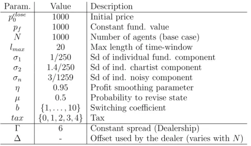
Table 1. Values of the parameters used in the

simula-tion, with short description.

Param. Value Description

pclose₀ 1000 Initial price

pf 1000 Constant fund. value

N 1000 Number of agents (base case)

lmax 20 Max length of time-window

σ1 1/250 Sd of individual fund. component

σ2 1.4/250 Sd of ind. chartist component

σn 3/1259 Sd of ind. noisy component

η 0.95 Profit smoothing parameter

µ 0.5 Probability to revise state

b {1, . . . ,10} Switching coefficient

tax {0,1,2,3,4} Tax

Γ 6 Constant spread (Dealership)

∆ - Offset used by the dealer (varies with N)

where U(1,∆) denotes a uniform sample in the interval[1,∆]. Hence the behaviour of the dealer is completely described by two parameters, namely the fixed spread Γ between quotes and ∆. The latter value will be tuned in the sequel to obtain time-series that are somehow comparable to the ones we got in a CDA.

Observe that in both CDA and Dea the price is not defined due to the presence of bids and asks. As in standard practice, whenever it is needed we consider the price to be the mid-point of outstanding quotes (or best bid, best ask).

4. _Results

We consider several computational experiments. Given a market pro-tocol, each experiment is a batch of 100 simulations (5000 trading days, discarding the first 500 to avoid transient effects), where all parameters are fixed with the exceptions of b andtax. This is meant to obtain 100 time series of 4500 returns, uniformly sampling b in {1,2, . . . ,10} and

taxin{0,1,2,3,4}in order to have representative data on a variety of settings with regard to the Tobin tax imposed on agents and on their profit sensitiveness.

The parameters used in the simulations are provided in Table 1. The values for the environmental and behavioural parameters are taken from the aforementioned CI paper in order to obtain realistic se-ries of returns. Most of the time sese-ries we generated show well known stylized facts like non-normal, fat tailed and non-autocorrelated re-turns. This is remarkable as the series are obtained with varying levels

We then consider three important indicators, namely volume, volatil-ity (standard deviation of log-returns) and distortion with respect to the fundamental value pf. The effects of the imposition of a specific

level of a TT can be estimated regressing the dependent variables vol-ume (volatility, distortion, respectively) against the independent vari-ables tax and b. In other words, we estimate the models

V olumei = k1+α taxi+β bi,

V olatilityi = k2+α taxi+β bi,

Distortioni = k3+α taxi+β bi,

using the whole sample (1 ≤ i ≤ 100) and the three subsamples for

which bi ∈ {1,2,3}, bi ∈ {4,5,6,7} and bi ∈ {8,9,10} corresponding

to strong, medium, low short-term profit sensitivity, respectively. It is useful to recall at this point the expected outcomes of a TT. The advocates of the imposition of a tax claim, with differentiated nuances, that this should decrease volatility, presumably deterring the most speculative traders to take part in the market. A reduction in volume should be observed together with more informative prices that might be more tightly linked to the fundamental values due to little excess volatility.

The following two subsections presents the results in a CDA and in a Dealership.

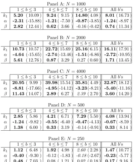
4.1. Continuos Double Auction (CDA). Table 2 exhibits the re-gression results for the volume in a CDA. As revealed in Panel A

(N = 1000 traders), an increase in the transaction tax reduces

vol-ume significantly. The reduction in volvol-ume is most pronounced when b

is low (-2.31 for b∈ {1,2,3} versus -0.87 forb ∈ {8,9,10}), a situation in which traders react quickly to transaction tax triggered changes in the profitability of their trading options. In addition, we see that vol-ume increases withb. Hence, ifb increases, more traders become active and thus volume grows. The other panels report findings for different

values of N. In particular, we see that if the number of traders

in-creases, the total volume increases and the impact of transaction taxes on volume becomes stronger. Only if the number of traders is very low

(N = 250, Panel E), the impact of transaction taxes on volume may

turn insignificant.

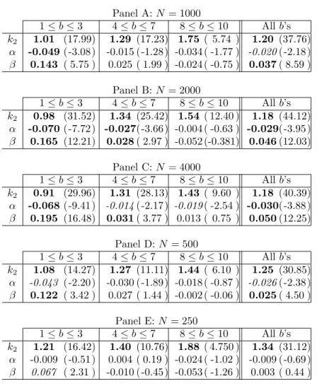
Table 3 shows how the results for the volatility in a CDA againsttax

and b, for different numbers of agents N and different subsamples with respect to b. The rightmost part of panel A shows that an unit incre-ment of the TT is decreasing the volatility by 0.02% (2 basis points), while the marginal effect of bis 0.037%. The decrement due to the tax is statistically significant at the 5% but not at the 1% confidence level. More importantly, the magnitude of the decrement is rather small in relative terms: given a volatility of the order of 100 basis points, a

Table 2. Volume in a CDA (units traded). The

esti-mates are relative to different numbers of agentsN (Pan-els A to E) and subsamples (low, medium, high, all b’s). Entries are in boldface (italic) if statistically significant at the 1% (5%) confidence level.

Panel A:N= 1000 1≤b≤3 4≤b≤7 8≤b≤10 Allb’s k1 5.20 ( 10.09 ) 9.24( 9.15 ) 14.80( 4.08 ) 8.01( 16.73 ) α -2.31 (-15.88) -1.21( -7.50 ) -0.87(-3.85) -1.24( -8.97 ) β 2.82 ( 12.44 ) 0.62( 3.66 ) -0.16 (-0.42) 0.74( 11.34 ) Panel B:N = 2000 1≤b≤3 4≤b≤7 8≤b≤10 Allb’s k1 10.73 ( 10.57 ) 22.72( 15.69 ) 25.16( 6.15 ) 16.11( 17.91 ) α -4.64 (-15.65) -2.74(-13.46) -1.51(-6.86) -2.72(-10.95) β 5.61 ( 12.76 ) 0.87( 3.29 ) 0.27 ( 0.60 ) 1.71( 13.45 ) Panel C:N = 4000 1≤b≤3 4≤b≤7 8≤b≤10 Allb’s k1 20.95 ( 9.99 ) 39.98( 15.54 ) 35.81( 4.49 ) 32.87( 18.12 ) α -8.81 (-17.66) -4.95(-14.12) -3.23(-8.21) -5.40(-11.16) β 11.43 ( 14.07 ) 2.89( 6.27 ) 2.39 ( 2.70 ) 3.60( 14.20 ) Panel D:N = 500 1≤b≤3 4≤b≤7 8≤b≤10 Allb’s k1 2.85 ( 5.86 ) 4.21( 6.71 ) 7.29( 5.50 ) 4.08( 13.94 ) α -1.24 ( -9.82 ) -0.55( -6.40 ) -0.47(-4.13) -0.67( -8.59 ) β 1.38 ( 6.00 ) 0.33( 3.19 ) -0.14 (-0.91) 0.33( 8.14 ) Panel E:N = 250 1≤b≤3 4≤b≤7 8≤b≤10 Allb’s k1 1.12 ( 6.48 ) 1.92( 4.98 ) 2.60 ( 2.28 ) 1.47( 10.77 ) α -0.40 ( -9.30 ) -0.12 ( -1.83 ) -0.18(-2.67) -0.23( -5.77 ) β 0.48 ( 7.03 ) 0.08 ( 1.21 ) 0.02 ( 0.18 ) 0.17( 9.16 )

reduction of 2 basis points might be considered negligible. Even in the

most reactive subsample (when 1 ≤b≤3) of simulations populated by

strongly profit-sensitive traders, the reduction is not exceeding 5 basis points (Panel A, leftmost part).

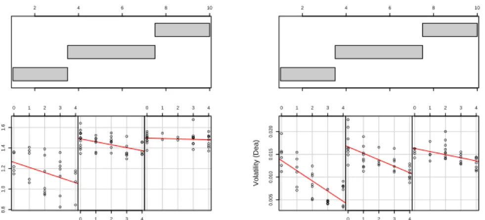
The same result is holding in markets with many agents, see Panels B and C: the tax has a slightly bigger effect and the coefficient is increasing from -0.020 to about -0.030 on the whole sample. Again, the leftmost part of the panels show increased efficacy for low b’s but still the achievable reduction of volatility appears to be rather small in relative terms. Figure 1 (left panel) depicts how the results (for

N = 2000) are dependent on the values of the parameter b, which is

related to short-term profit sensitivity. In agreement with intuition, the effectiveness of the tax is visibly bigger for small values of b.

● ● ● ● ● ● ● ● ● ● ● ● ● ● ● ● ● ● ● ● ● ● ● ● ● ● ● ● 0 1 2 3 4 0.8 1.0 1.2 1.4 1.6 ● ● ● ● ● ● ● ● ● ● ● ● ●● ● ● ● ● ● ● ● ● ● ● ● ● ● ● ● ● ● ● ● ● ● ● ● ● ● ● 0 1 2 3 4 ● ● ● ● ● ● ● ● ● ● ● ● ● ● ● ● ● ●● ● ● ● ● ● ● ● ● ● ● ● ● ● 0 1 2 3 4 Tax Volatility (CDA) 2 4 6 8 10 Given : b ● ● ● ● ● ●●●●●●● ●● ● ● ● ● ● ● ● ● ● ● ● ● ● ● ● ● ● ● ● ● 0 1 2 3 4 0.005 0.010 0.015 0.020 ● ● ● ● ● ● ● ●● ● ● ● ● ● ● ● ● ● ● ● ● ● ● ● ● ● ● ● ● ● ● ● ● ● ● 0 1 2 3 4 ● ● ● ● ● ● ● ● ● ● ● ● ● ● ● ● ● ● ● ● ● ● ● ● ● ● ● ● ● ● ● 0 1 2 3 4 Tax Volatility (Dea) 2 4 6 8 10 Given : b

Figure 1. Volatility in a CDA and in a Dealership with

2000 agents, for b ∈ {1,2,3},{4,5,6,7},{8,9,10} (from left to right).

Moreover, markets with few agents (Table 3, Panel D and E) are “thin” and there is little evidence of statistically significant effects, if any. Additional comments on the importance of liquidity are deferred to the following subsection.

Table 4 presents the regression results obtained for the (percent) dis-tortion, a measure of deviation from the fundamental value computed as 100 N N X t=1 pt−pf pf .

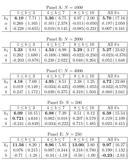
Despite the common claim that a Tobin tax might help in reducing the distortion, we find no support for this effect. Figure 2 (left panel)

depicts the situation in a CDA with N = 1000 agents. It’s clear that

a TT is unable to reduce the distortion and, in some cases, appears to mildly increase the deviation from the fundamental.

4.2. Dealership. In this section we examine the effect of a TT in a dealership, according to the same measures (volume, volatility and distortion) used in a CDA. We keep fixed the behaviour of the traders, changing the market. The experiment is meant to test weather the results are stable across different microstructures and, in particular, if the addition of an exogenous liquidity source (the dealer) is altering our

findings. We keep Γ = 6 (constant bid-ask spread) and vary ∆ = ∆(N)

(variation of quote) depending on the number of agents, in such a way to get a volatility of the same order of CDA. We stress that this “calibration” exercise is hard and imperfect as we try to align 100 time-series (one for each simulation) obtained across different parameters in institutionally different markets. By trial and error we get values for ∆ such that the average volatility in a dealership is similar but

Table 3. Volatility in a CDA (%). The estimates are

relative to different numbers of agents N (Panels A to

E) and subsamples (low, medium, high, all b’s). Entries are in boldface (italic) if statistically significant at the 1% (5%) confidence level. Panel A:N= 1000 1≤b≤3 4≤b≤7 8≤b≤10 Allb’s k2 1.01 (17.99) 1.29 (17.23) 1.75( 5.74 ) 1.20 (37.76) α -0.049(-3.08) -0.015 (-1.28) -0.034 ( -1.77 ) -0.020(-2.18) β 0.143 ( 5.75 ) 0.025 ( 1.99 ) -0.024 ( -0.75 ) 0.037( 8.59 ) Panel B:N = 2000 1≤b≤3 4≤b≤7 8≤b≤10 Allb’s k2 0.98 (31.52) 1.34 (25.42) 1.54( 12.40 ) 1.18 (44.12) α -0.070(-7.72) -0.027(-3.66) -0.004 ( -0.63 ) -0.029(-3.95) β 0.165 (12.21) 0.028( 2.97 ) -0.052 (-0.381) 0.046(12.03) Panel C:N = 4000 1≤b≤3 4≤b≤7 8≤b≤10 Allb’s k2 0.91 (29.96) 1.31 (28.13) 1.43( 9.60 ) 1.18 (40.39) α -0.068(-9.41) -0.014(-2.17) -0.019( -2.54 ) -0.030(-3.88) β 0.195 (16.48) 0.031( 3.77 ) 0.013 ( 0.75 ) 0.050(12.25) Panel D:N = 500 1≤b≤3 4≤b≤7 8≤b≤10 Allb’s k2 1.08 (14.27) 1.27 (11.11) 1.44( 6.10 ) 1.25 (30.85) α -0.043 (-2.20) -0.030 (-1.89) -0.018 ( -0.87 ) -0.026(-2.38) β 0.122 ( 3.42 ) 0.027 ( 1.44 ) -0.002 ( -0.06 ) 0.025( 4.50 ) Panel E:N = 250 1≤b≤3 4≤b≤7 8≤b≤10 Allb’s k2 1.21 (16.42) 1.40 (10.76) 1.88( 4.750 ) 1.34 (31.12) α -0.009 (-0.51) 0.004 ( 0.19 ) -0.024 ( -1.02 ) -0.009 (-0.69) β 0.067 ( 2.31 ) -0.010 (-0.45) -0.053 ( -1.26 ) 0.003 ( 0.44 )

never exceeding the average value in the “parallel” CDA. It turns out that this volatility-based calibration also allows to get roughly similar volumes and distortions in the two markets. Table 5 shows descriptive statistics of the volatility in the two markets for various sizes of traders’ population.

A look at the table reveals that at least 75% of the simulations (be-tween the first and third quartile) in each panel are close in terms of volatility. The average standard deviations of returns in a CDA and in a dealership rarely differ by more than 20 basis points, despite wider differences in some extreme occasions. Read with some liberty, Table 5

Table 4. Distortion in a CDA (%). The estimates are

relative to different numbers of agents N (Panels A to

E) and subsamples (low, medium, high, all b’s). Entries are in boldface (italic) if statistically significant at the 1% (5%) confidence level. Panel A:N= 1000 1≤b≤3 4≤b≤7 8≤b≤10 Allb’s k3 6.10 ( 7.71 ) 5.36( 6.75 ) 6.97 ( 2.00 ) 5.70( 17.16 ) α 0.260 ( 1.165 ) 0.301( 2.378 ) -0.011(-0.050) 0.197( 2.050 ) b -0.228 (-0.655) 0.019 ( 0.145 ) -0.085(-0.231) 0.007 ( 0.161 ) Panel B:N = 2000 1≤b≤3 4≤b≤7 8≤b≤10 Allb’s k3 5.23 ( 9.81 ) 4.53( 6.99 ) 5.29( 3.17 ) 5.27( 23.62 ) α 0.262 ( 1.680 ) -0.169(-1.860) -0.022(-0.250) -0.023(-0.376) b -0.203 (-0.878) 0.238 ( 2.022 ) 0.048 ( 0.264 ) 0.052 ( 1.648 ) Panel C:N = 4000 1≤b≤3 4≤b≤7 8≤b≤10 Allb’s k3 4.18 ( 7.69 ) 4.95( 8.51 ) 2.38 ( 1.25 ) 4.72( 22.60 ) α 0.019 ( 0.149 ) -0.034(-0.435) -0.099(-1.055) -0.032(-0.579) b 0.247 ( 1.172 ) 0.039 ( 0.375 ) 0.319 ( 1.503 ) 0.060( 2.041 ) Panel D:N = 500 1≤b≤3 4≤b≤7 8≤b≤10 Allb’s k3 6.09 ( 10.15 ) 6.98( 7.39 ) 0.51 ( 0.12 ) 6.38( 15.54 ) α 0.721( 4.616 ) 0.002 ( 0.018 ) 0.207 ( 0.570 ) 0.229( 2.109 ) b -0.241 (-0.849) -0.034(-0.222) 0.715 ( 1.485 ) 0.023 ( 0.415 ) Panel E:N = 250 1≤b≤3 4≤b≤7 8≤b≤10 Allb’s k3 11.56( 8.20 ) 9.96( 5.95 ) 13.00( 2.80 ) 9.97( 16.27 ) α 0.076 ( 0.215 ) 0.097 ( 0.344 ) 0.218 ( 0.780 ) 0.199 ( 1.132 ) b -0.71 ( -1.28 ) -0.34 ( -1.19 ) -0.50 ( -1.00 ) -0.23( -2.83 )

justifies the claim that we can reasonably compare across different mar-kets the effects of the introduction of a TT, given that the simulations produced are, to the best of our efforts, quite similar1

.

Table 4.2 contains the results of the regression of the volatility in a dealership against the usual independent variables tax, band is exactly homologous with Table 3. The marginal effect of the TT is strongly statistically significant even in thin markets (Panels D and E). Ob-serve that this holds despite the fact that there is “less to reduce” in

1_{Observe that we calibrate a single parameter in the dealership, ∆, to “match” a}

single average value for the volatility in a CDA. Table 5, however, shows a com-parison of two distributions of values. Even forgetting the deep differences between the two market clearing mechanisms, it’s not surprising that a closer match is hard to get.

● ● ● ● ● ● ● ● ● ● ● ●● ● ● ● ● ● ● ● ● ● ● ● ● ● ● ● ● 0 1 2 3 4 4 5 6 7 8 9 10 ● ● ● ● ● ● ● ● ● ● ● ● ● ● ● ● ● ● ● ● ● ● ● ● ● ● ● ● ● ● ● ● ● ● ● ● ● ● ● ● ● ● ● ● ● ● ● ● 0 1 2 3 4 ● ● ● ● ● ● ● ● ● ● ● ● ● ● ● ● ● ● ● ● ● ● ● 0 1 2 3 4 Tax Distortion (CDA) 2 4 6 8 10 Given : b ● ● ● ● ● ● ● ● ● ● ● ● ● ● ● ● ● ● ● ● ● 0 1 2 3 4 5 10 15 20 ● ● ● ● ● ● ● ● ● ● ● ● ● ● ● ● ● ● ● ● ● ● ● ● ● ● ● ● ● ● ● ● ● ● 0 1 2 3 4 ● ● ● ● ● ● ● ● ● ● ● ● ● ● ● ● ● ● ● ● ● ● ● ● ● ● ● ● ● ● ● ● ● ● ● ● ● ● ● ● ● ● ● ● ● 0 1 2 3 4 Tax Distortion (Dea) 2 4 6 8 10 Given : b

Figure 2. Distortion in a CDA and in a dealership as

functions of tax, given b.

Table 5. Comparison of volatilities (%) obtained in a

CDA and in a Dealership with the same number of agents

N. The parameter ∆ varies to get comparable volatility

with the CDA over the whole sample.

Panel A:N = 1000,∆ = 6

Min. 1Qu. Median Mean 3Qu. Max. CDA 0.954 1.286 1.384 1.367 1.478 1.694 Dea 0.4782 1.0710 1.1840 1.1720 1.2750 1.8300

Panel B:N = 2000,∆ = 4

Min. 1Qu. Median Mean 3Qu. Max. CDA 0.8261 1.3400 1.4340 1.3780 1.5000 1.6760

Dea 0.3434 1.0250 1.3090 1.2480 1.5290 2.2630 Panel C: N= 4000,∆ = 2.25

Min. 1Qu. Median Mean 3Qu. Max. CDA 0.8111 1.3320 1.4380 1.3880 1.5000 1.6370

Dea 0.4153 1.0850 1.2820 1.2400 1.4590 1.9470 Panel D:N = 500,∆ = 11

Min. 1Qu. Median Mean 3Qu. Max. CDA 0.9784 1.2310 1.3140 1.3360 1.4480 1.9100

Dea 0.4295 1.1190 1.2720 1.2710 1.4270 2.0640 Panel E:N = 2000,∆ = 15

Min. 1Qu. Median Mean 3Qu. Max. CDA 1.024 1.229 1.347 1.337 1.434 1.925 Dea 0.5837 1.0190 1.1290 1.1380 1.2430 1.8290

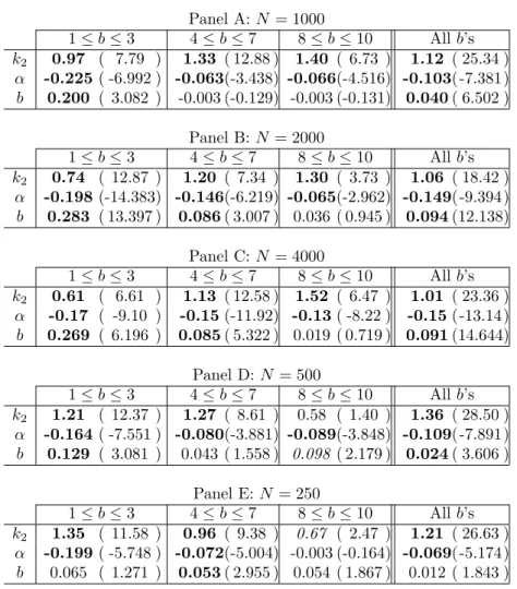
Table 6. Volatility in a Dealership (%). The estimates

are relative to different numbers of agentsN (Panels A to E) and subsamples (low, medium, high, all b’s). Entries are in boldface (italic) if statistically significant at the 1% (5%) confidence level. Panel A:N= 1000 1≤b≤3 4≤b≤7 8≤b≤10 Allb’s k2 0.97 ( 7.79 ) 1.33 ( 12.88 ) 1.40 ( 6.73 ) 1.12 ( 25.34 ) α -0.225( -6.992 ) -0.063(-3.438) -0.066(-4.516) -0.103(-7.381) b 0.200 ( 3.082 ) -0.003 (-0.129) -0.003 (-0.131) 0.040( 6.502 ) Panel B:N = 2000 1≤b≤3 4≤b≤7 8≤b≤10 Allb’s k2 0.74 ( 12.87 ) 1.20 ( 7.34 ) 1.30 ( 3.73 ) 1.06 ( 18.42 ) α -0.198(-14.383) -0.146(-6.219) -0.065(-2.962) -0.149(-9.394) b 0.283 ( 13.397 ) 0.086( 3.007 ) 0.036 ( 0.945 ) 0.094(12.138) Panel C:N = 4000 1≤b≤3 4≤b≤7 8≤b≤10 Allb’s k2 0.61 ( 6.61 ) 1.13 ( 12.58 ) 1.52 ( 6.47 ) 1.01 ( 23.36 ) α -0.17 ( -9.10 ) -0.15(-11.92) -0.13( -8.22 ) -0.15(-13.14) b 0.269 ( 6.196 ) 0.085( 5.322 ) 0.019 ( 0.719 ) 0.091(14.644) Panel D:N = 500 1≤b≤3 4≤b≤7 8≤b≤10 Allb’s k2 1.21 ( 12.37 ) 1.27 ( 8.61 ) 0.58 ( 1.40 ) 1.36 ( 28.50 ) α -0.164( -7.551 ) -0.080(-3.881) -0.089(-3.848) -0.109(-7.891) b 0.129 ( 3.081 ) 0.043 ( 1.558 ) 0.098 ( 2.179 ) 0.024( 3.606 ) Panel E:N = 250 1≤b≤3 4≤b≤7 8≤b≤10 Allb’s k2 1.35 ( 11.58 ) 0.96 ( 9.38 ) 0.67 ( 2.47 ) 1.21 ( 26.63 ) α -0.199( -5.748 ) -0.072(-5.004) -0.003 (-0.164) -0.069(-5.174) b 0.065 ( 1.271 ) 0.053( 2.955 ) 0.054 ( 1.867 ) 0.012 ( 1.843 )

a dealership whose (average) volatility is never bigger than in a CDA. More fundamentally from a practical point of view, the trimming of the volatility is amplified by a factor of 5 or more on the whole sample (see the “All b’s” parts). Virtually all subsamples show that a size-able reduction is possible imposing low levels of taxation (tax = 1,2 roughly equivalent to 0.1-0.2% proportional taxation rate) that are re-cently hypothesized in the debate on this topic. The right panel of Figure 1 shows the reduction of volatility when N = 2000, for different values of b.

As far as volume and distortion are concerned, we provide in Appen-dix B Tables 9 and 8 with full regression results.

Similarly to what observed in a CDA, the volume is strongly affected in a dealership. Observe that this is providing further support to the

observation that reducing the volatility is not tantamount to volume cutting. Hence, if a TT is visibly decreasing the volume in both CDA’s and dealerships, some other driver is responsible for the different out-comes in terms of volatility. A first, perhaps trivial, explanation lies in the different role taken by the bid-ask spread in the two markets. While a reduction in the traded volume is likely to widen the bid-ask spread in a CDA, one of the features of our dealership is that a constant bid-ask is provided to the dealer at any time. This liquidity provision is not affected by the number of transactions, given the duty for the dealer to quote prices with no discontinuity. Second, a careful inspection of the data shows that smaller volume produce sparse orders’ books in a CDA. A sequence of marketable limit orders of the same type can then escalate the book producing wide price changes. These liquidity holes are, by definition, missing in a dealership and this results in smoother price dynamics under reduced volume. Somewhat related comments on microstructures have been given, for example, in [10], [19] and [18]. The imposition of a tax in a Dealership has again a somewhat weak (and often null) effect on distortion, see also Figure 2, right panel.

5. Conclusion

In this paper, we explore the effectiveness of transaction taxes in dif-ferent institutional market microstructure settings. Within our model, asset prices are driven by the orders of the market participants. These agents rely on technical, fundamental and random trading strategies to determine their investment positions. However, they are not forced to trade. The decision to be active or inactive depends on the past prof-itability of the agent’s trades. Should a trader encounter losses, he/she may decide to stop trading (and vice versa). In one of our scenarios, the orders of the market participants enter a continuous double auction market. In another scenario, the orders of the market participants are filled by a specialist. Both settings are, in general, able to mimic some stylized facts of financial markets and thus allow a comparison of the impact of transaction taxes on the market dynamics.

Our key findings may be summarized as follows:

• In a continuous double auction market, the imposition of a

transaction has presumably no stabilizing impact on the market dynamics. We observe that traders retreat from the market if a levy has to be paid and that thus volume decreases. How-ever, also liquidity decreases so that on average a given order obtains a larger price impact. This, in turn, counters or even eliminates an otherwise stabilizing effect of the transaction tax. The distortion in the market remains unaltered.

• Our model predicts that in a dealership market a transaction

environment, traders retreat from the market and volume de-clines. However, since liquidity is exogenously provided by a specialist the price impact of a given order remains constant and thus volatility significantly declines. Surprisingly, the dis-tortion is not significantly reduced.

Summing up, we find that market microstructure details matter for the effectiveness of transaction taxes. We hope that our paper resolves some of the confusion frequently observed in the debate on the nature of transaction taxes.

References

[1] Aliber, R., Chowdhry, B. and Yan, S. (2003): Some evidence that a Tobin tax on foreign exchange transaction may increase volatility. European Finance Review, 7, 481-510.

[2] Brock, W. and Hommes, C. (1998): Heterogeneous beliefs and routes to chaos in a simple asset pricing model. Journal of Economic Dynamics Control, 22, 1235-1274.

[3] Chiarella, C. (1992): The dynamics of speculative behavior. Annals of Opera-tions Research, 37, 101-123.

[4] Chiarella, C. and Iori, G (2002): A Simulation Analysis of the Microstructure of Double Auction Markets, Quantitative Finance, 2, 5, 346-353.

[5] Day, R. and Huang, W. (1990): Bulls, bears and market sheep. Journal of Economic Behavior and Organization, 14, 299-329.

[6] De Grauwe, P., Dewachter, H. and Embrechts, M. (1993): Exchange rate theory – chaotic models of foreign exchange markets. Blackwell, Oxford. [7] Ehrenstein, G., Westerhoff, F. and Stauffer, D. (2005): Tobin tax and market

depth. Quantitative Finance, 5, 213-218.

[8] Eichengreen, B., Tobin, J. and Wyplosz, C. (1995): Two cases for and in the wheels of international finance. Economic Journal, 105, 162-172.

[9] Farmer, D. and Joshi, S. (2002): The price dynamics of common trading strate-gies. Journal of Economic Behavior and Organization, 49, 149-171.

[10] Farmer, D., Gillemot, L. , Lillo, F., Mike, S. and A. Sen (2004): What Really Causes Large Price Changes? Quant. Fin. 4, 4, 383-397.

[11] Frankel, J. (1996): How well do foreign exchange markets function: Might a Tobin tax help? NBER Working Paper 5422.

[12] Hau, H. (2006): The role of transaction costs for financial volatility: Evidence from the Paris bourse. Journal of the European Economic Association, 4, 862-890.

[13] Hommes, C. (2006): Heterogeneous agent models in economics and finance. In: Tesfatsion, L. and Judd, K. (eds.): Handbook of computational economics Vol. 2: Agent-based computational economics. North-Holland, Amsterdam, 1107-1186.

[14] Jones, C. and Seguin, P. (1997): Transaction costs and price volatility: Evi-dence from commission deregulation. American Economic Review, 87, 728-737. [15] Keynes, J.M. (1936): The general theory of employment, interest, and money.

Harcourt Brace, New York.

[16] Kirman, A. (1991): Epidemics of opinion and speculative bubbles in finan-cial markets. In: Taylor, M. (Ed.): Money and finanfinan-cial markets. Blackwell, Oxford, 354-368.

[17] LeBaron, B. (2006): Agent-based computational finance. In: Tesfatsion, L. and Judd, K. (Eds.): Handbook of computational economics Vol. 2: Agent-based computational economics. North-Holland, Amsterdam, 1187-1233.

[18] Lillo, F., Farmer, D. and Mantegna, R. (2003): Single Curve Collapse of the Price Impact Function for the New York Stock Exchange. Nature, 421, 129-130. [19] Lillo, F. and Farmer D. (2005): The Key Role of Liquidity Fluctuations in De-termining Large Price Fluctuations. Fluctuations and Noise Letters, 5, L209-L216.

[20] Lux, T. (1995): Herd behavior, bubbles and crashes. Economic Journal, 105, 881-896.

[21] Lux, T. (2006): Financial power laws: Empirical evidence, models and mecha-nisms. In. Cioffi-Revilla, C. (ed.): Power laws in the social sciences: Discovering complexity and non-equilibrium dynamics in the social universe, in press. [22] Mannaro, K., Marchesi, M. and Setzu, A. (2006): Using an artificial financial

market for assessing the impact of Tobin-like transaction taxes. Journal of Economic Behavior and Organization, in press.

[23] Maslov, S. (2000): Simple model of a limit order-driven market. Physica A 278, 571–578.

[24] Pellizzari, P. and Dal Forno, A. (2007): A comparison of different trading protocols in an agent-based market, Journal of Economic Interaction and Co-ordination, 2, n. 1, 27–43.

[25] Rosser, J. Jr., Ahmed, E. and Hartmann, G. (2003): Volatility via social flaring, Journal of Economic Behavior & Organization, 50, 77-87.

[26] Schwert, W. and Seguin, P. (1993): Securities transaction taxes: An overview of costs, benefits and unresolved questions. Financial Analyst Journal, 49, 27-35.

[27] Shiller, R. (2000): Irrational exuberance. Princeton University Press, Prince-ton.

[28] Spahn, B. (2002): On the feasibility of a tax on foreign exchange transactions. Report commissioned by the Federal Ministry for Economic Cooperation and Development, Bonn.

[29] Stiglitz, J. (1989): Using tax policy to curb speculative short-term trading. Journal of Financial Services, 3, 101-113.

[30] Summers, L. and Summers, V. (1989): When financial markets work too well: A cautious case for a securities transaction tax. Journal of Financial Services, 3, 163-188.

[31] Taylor, M. and Allen, H. (1992): The use of technical analysis in the foreign exchange market. Journal of International Money and Finance, 11, 304-314. [32] Tobin, J. (1978): A proposal for international monetary reform. Eastern

Eco-nomic Journal, 4, 153-159.

[33] Ul Haq, M., Kaul, I. and Grunberg, I. (1996): The Tobin tax: Coping with financial volatility. Oxford University Press, New York.

[34] Umlauf, S. (1993): Transaction taxes and the behavior of the Swedish stock market. Journal of Financial Economics, 33, 227-240.

[35] Werner, I. (2003): Comment on ’Some Evidence that a Tobin Tax on Foreign Exchange Transactions may Increase Volatility’. European Finance Review, 7, 511-514.

[36] Westerhoff, F. (2003): Heterogeneous traders and the Tobin tax. Journal of Evolutionary Economics, 13, 53-70.

[37] Westerhoff, F. and Dieci, R. (2006): The effectiveness of Keynes-Tobin trans-action taxes when heterogeneous agents can trade in different markets: A

behavioral finance approach. Journal of Economic Dynamics and Control, 30, 293-322.

Appendix A. Stylized facts

This appendix aims to describe the time series that are analyzed in the paper corroborating the claim that our model is able, despite its simplicity, to produce reasonably realistic returns. We show in the following that the data exhibit some among the common statistical features of financial time-series that are frequently dubbed “stylized facts”. For brevity, we comment in this Appendix only the simulations with 1000 agents in a CDA and 2000 in a Dealership.

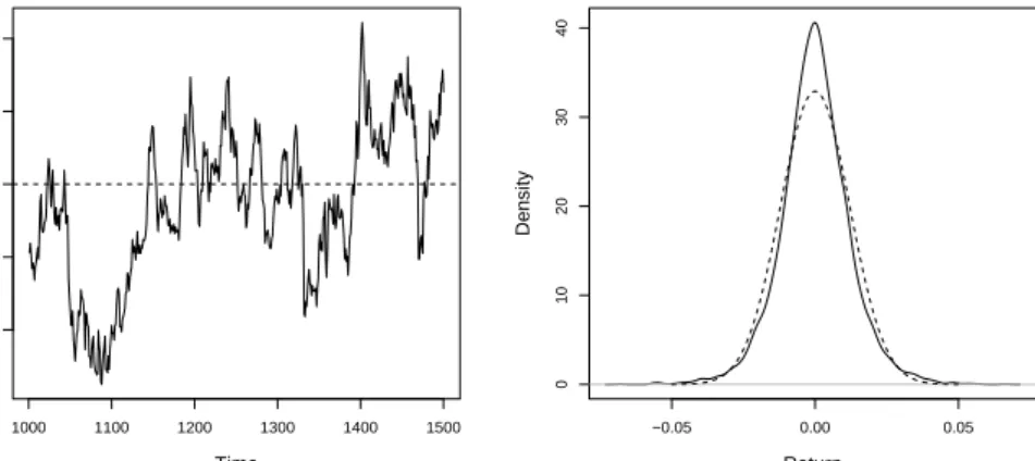
Figure 3 depicts a representative price trajectory in a CDA, to-gether with the density of the log-returns. The price visually displays a random-like behaviour with sudden bursts and crashes. The density is clearly non-gaussian, leptokurtic and fat-tailed. Formal tests reveals

1000 1100 1200 1300 1400 1500 900 950 1000 1050 1100 Time Midprice −0.05 0.00 0.05 0 10 20 30 40 Return Density

Figure 3. Price time series and returns’ density of a

representative CDA simulation (N = 1000, b = 9, tax = 4). The dashed lines show the fundamental value (left) and a normal distribution with same mean and variance (right).

that normality can be strongly rejected and lagged returns are indepen-dent (the Shapiro-Wilk p-value is smaller than 10−20_{; the Box-Pierce}

p-value with 5 lags is 0.60, so that independence cannot be rejected). This example is somewhat illustrative of the whole sample obtained when the market is a CDA: normality of returns is (strongly) rejected for all simulations and the null hypothesis of linear independence of returns is rejected at the 1% confidence level by Box-Pierce test in 8 cases out of 100.

The simulated returns in CDA show a fair amount of excess kurtosis (with respect to the gaussian valueµ4 = 3), see the upper part of Table

Table 7. Descriptive statistics for the kurtosis

(normal-ized central fourth moment) of returns in a CDA and in a Dealership.

Min. 1Qu. Median Mean 3Qu. Max.

CDA (N = 1000) 3.910 4.450 4.743 4.855 5.178 7.334

Dea (N = 2000) 2.574 2.897 3.022 3.059 3.121 4.564

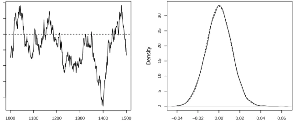
The time series obtained in a Dealership are slightly less satisfactory in that returns are closer to normality and there is a weak degree of linear predictability in some cases. The observation that some market mechanisms (like the CDA) may make the presence of stylized facts more likely is not new, see [24] and [23]. Figure 4 shows a representative example of price and returns’ density. The price is fluctuating quite realistically, with pronounced deviations from the fundamental. The hypothesis of normal distribution of returns cannot be rejected (the p -value is 0.075) confirming the visual proximity of the densities displayed on the right part of Figure 4. Examining the whole sample, normality

1000 1100 1200 1300 1400 1500 800 850 900 950 1000 1050 1100 Time Midprice −0.04 −0.02 0.00 0.02 0.04 0.06 0 5 10 15 20 25 30 Return Density

Figure 4. Price time series and returns’ density of

a typical simulation in a Dealership (N = 2000, b =

9, tax = 4). The dashed lines show the fundamental

value (left) and a normal distribution with same mean and variance (right).

is rejected at the 5% confidence level by a Shapiro-Wilk in 54 cases out of 100. As seen in the lower part of Table 7, there is little evidence of excess kurtosis when the market platform is a Dealership.

The independence of returns is not rejected (at the 1% level) for 78 simulations. In the 22 cases where some linear structure is present in the returns, the strength of predictability is extremely low. Figure 5 depicts, for every simulation, the autocorrelation with biggest modulus (35 lags are considered).

0 20 40 60 80 100 −0.08 −0.06 −0.04 −0.02 0.00 0.02 0.04 Simulation Extreme autocorration

Figure 5. Autocorrelation with biggest absolute value,

for each of the 100 simulations of a Dealership withN = 2000 agents.

On the one hand, the absolute magnitude of the autocorrelation is rarely exceeding 0.05: this predictability is statistically significant, at times but is rather low to provide trading gains. On the other hand, the prevalence of negative signs in the picture is suggesting that this weak autocorrelation might be due to the bid-ask bounce possibly occurring in a Dealership.

Appendix B. Dealership’s data

This appendix shows the regression results for the volume (Table 8) and the distortion (Table 9) in a Dealership market.

Table 8. Volume in a Dealership (units traded). The

estimates are relative to different numbers of agents N

(Panels A to E) and subsamples (low, medium, high, all b’s). Entries are in boldface (italic) if statistically significant at the 1% (5%) confidence level.

Panel A:N= 1000 1≤b≤3 4≤b≤7 8≤b≤10 Allb’s k1 7.63 ( 5.80 ) 12.02( 9.02 ) 14.55( 5.98 ) 9.79( 18.40 ) α -2.85 ( -8.37 ) -0.82( -3.42 ) -0.92( -5.40 ) -1.36( -8.02 ) b 2.76 ( 4.03 ) 0.12 ( 0.48 ) -0.07 ( -0.27 ) 0.59( 7.96 ) Panel B:N = 2000 1≤b≤3 4≤b≤7 8≤b≤10 Allb’s k1 9.06 ( 9.34 ) 17.75( 7.20 ) 23.06( 4.15 ) 14.53( 14.43 ) α -3.72 (-16.07) -2.64( -7.48 ) -1.01( -2.87 ) -2.69( -9.65 ) b 5.26 ( 14.85 ) 1.64( 3.80 ) 0.31 ( 0.51 ) 1.86( 13.70 ) Panel C:N = 4000 1≤b≤3 4≤b≤7 8≤b≤10 Allb’s k1 11.85( 4.07 ) 34.14( 15.99 ) 43.55( 9.00 ) 27.59( 18.84 ) α -6.34 (-11.01) -4.59(-15.52) -3.87(-12.27) -4.84(-12.83) b 10.94( 8.01 ) 2.63( 6.91 ) 0.94 ( 1.74 ) 3.33( 15.92 ) Panel D:N = 500 1≤b≤3 4≤b≤7 8≤b≤10 Allb’s k1 5.79 ( 8.62 ) 6.19( 5.73 ) 3.68 ( 1.40 ) 6.84( 20.52 ) α -1.22 ( -8.18 ) -0.64( -4.24 ) -0.57( -3.89 ) -0.80( -8.31 ) b 0.92 ( 3.20 ) 0.35 ( 1.71 ) 0.42 ( 1.48 ) 0.18( 3.77 ) Panel E:N = 250 1≤b≤3 4≤b≤7 8≤b≤10 Allb’s k1 4.68 ( 7.45 ) 3.31( 5.94 ) 1.07 ( 0.72 ) 4.37( 17.43 ) α -1.21 ( -6.48 ) -0.54( -6.94 ) -0.09 ( -0.88 ) -0.49( -6.67 ) b 0.60 ( 2.16 ) 0.26 ( 2.66 ) 0.32 ( 2.03 ) 0.07 ( 1.90 )

Table 9. Distortion in a Dealership (%). The estimates

are relative to different numbers of agentsN (Panels A to E) and subsamples (low, medium, high, all b’s). Entries are in boldface (italic) if statistically significant at the 1% (5%) confidence level. Panel A:N= 1000 1≤b≤3 4≤b≤7 8≤b≤10 Allb’s k3 5.56 ( 3.85 ) 5.81( 3.09 ) 8.52 ( 1.62 ) 7.41( 11.02 ) α -0.50 ( -1.34 ) -0.20 ( -0.58 ) -0.51 ( -1.40 ) -0.42 ( -1.96 ) b 1.553 ( 2.067 ) 0.357 ( 1.019 ) 0.077 ( 0.129 ) 0.175 ( 1.868 ) Panel B:N = 2000 1≤b≤3 4≤b≤7 8≤b≤10 Allb’s k3 7.49 ( 9.23 ) 5.81( 6.55 ) 4.22 ( 1.23 ) 6.28( 16.47 ) α 0.201 ( 1.036 ) -0.242(-1.903) 0.110 ( 0.507 ) 0.033 ( 0.311 ) b -0.738 (-2.493) 0.122 ( 0.787 ) 0.232 ( 0.614 ) -0.008(-0.145) Panel C:N = 4000 1≤b≤3 4≤b≤7 8≤b≤10 Allb’s k3 6.60 ( 7.57 ) 5.11( 7.84 ) 5.38( 4.56 ) 5.26( 20.96 ) α 0.09 ( 0.52 ) -0.14 ( -1.59 ) -0.34( -4.49 ) -0.16( -2.43 ) b -0.938 (-2.292) 0.055 ( 0.475 ) 0.066 ( 0.499 ) 0.033 ( 0.920 ) Panel D:N = 500 1≤b≤3 4≤b≤7 8≤b≤10 Allb’s k3 9.43 ( 4.31 ) 8.68( 3.84 ) 17.39 ( 1.40 ) 9.38( 9.93 ) α -0.163 (-0.334) -0.179(-0.567) 0.269 ( 0.390 ) -0.046(-0.169) b 0.028 ( 0.030 ) 0.209 ( 0.493 ) -0.948(-0.706) 0.001 ( 0.005 ) Panel E:N = 250 1≤b≤3 4≤b≤7 8≤b≤10 Allb’s k3 14.13 ( 4.60 ) 20.30( 3.28 ) 5.21 ( 1.39 ) 14.90( 10.19 ) α -1.62 ( -1.78 ) -0.79 ( -0.91 ) -0.36 ( -1.45 ) -0.86( -2.02 ) b 0.24 ( 0.17 ) -1.22 ( -1.13 ) 0.48 ( 1.20 ) -0.40( -1.99 )

Ca’ Foscari University, Dept. of Applied Mathematics, Dorsuduro 3825/E, 30123 Venice - Italy

E-mail address: [email protected]

University of Bamberg, Department of Economics, Feldkirchenstrasse 21, 96045 Bamberg - Germany