Distribution
control
79
Distribution control
at Exhaust Systems Europe
Sander de Leeuw
Department of International Distribution/Logistics, School of
Technology Management, Eindhoven University of Technology,
Eindhoven, The Netherlands
Introduction: the necessity for additional logistics control theory
Physical distribution control is concerned with all activities needed to co-ordinate the place and timing of demand for and supply of products and capacities in such a way that objectives regarding products, markets, and the distribution process are met[1]. The way distribution activities are controlled in a company is represented in a distribution control technique, which comprises decisions regarding the method used for replenishing and allocating inventory in physical distribution systems.
Several standard techniques for physical distribution control have been developed and applied. A classic technique is the reorder point (ROP) technique. According to ROP, each warehouse orders a batch – fixed or variable in size – each time a prespecified inventory level is passed. The level of this so called reorder point is dependent on variables such as the mean and deviation of the supply lead time and the mean and deviation of the demand rate. In more advanced systems, orders are placed when echelon inventory levels – i.e. the inventory of the warehouse considered plus the inventory in all its downstream warehouses – instead of local (also called installation) stock levels are passed. Base stock control is an example of such a technique that uses echelon stock norms (see, for example, Silver and Peterson[2]). More recent techniques use replenishments that are not triggered by realizations of customer demand (reactive) but by future demand forecasts (proactive). Again, replenishments can be based on either local stock norms (distribution requirements planning) or on integral stock norms (line requirements planning[3]).
Very often, the literature introducing new concepts in the area of distribution as well as production does not discuss application restrictions, as can be seen in the work by Martin[4], Orlicky[5] or Goldratt and Cox[6]. Theoretical and practical evidence, however, shows that the application of these standard control techniques is not always equally successful[3,7,8]. Only a few attempts have been made so far to assess the applicability of distribution control techniques[7,8]. Moreover, in the literature, it is hardly discussed how physical
Received August 1995 Revised February 1996 Revised May 1996
International Journal of Physical Distribution & Logistics Management, Vol. 26 No. 8, 1996, pp. 79-96. © MCB University Press, 0960-0035
The author is grateful to Kees van der Snel, his Master's thesis was the basis for this article. Futhermore, he would like to thank Thierry Verduijn and Dr Karel van Donselaar for reading and commenting on earlier versions of this article. This research was sponsored by the Technology Foundation (STW).
IJPDLM
26,8
80
distribution control techniques should be selected. Co-ordination between business functions, for example the co-ordination between distribution and production, is often not part of the scope of a distribution control framework. It was therefore judged necessary to enlarge the knowledge on the successful application of physical distribution control techniques. The case study described in this article has been carried out as part of a PhD project[9], which is concerned with finding relevant factors for the selection of physical distribution control techniques and with investigating how these factors affect this selection. The goal of the study is to draw conclusions based on the relationship between, on the one hand, company and environmental characteristics, and on the other, the selection of distribution control techniques. This article introduces a method for selecting a physical distribution control framework by describing a case study which has been worked out with this method. It should be noted that commercial aspects of distribution, such as the choice of the distribution channel, are not subject of research. The reader should read physical distribution every time the word “distribution” is used.
Basics for choosing a control technique
In distribution control design, we adhere to two design principles. The first design principle is called “contingency”. Contingency theory has been widely applied in management science and states that a system will only be effective if there is a balance between this system and its relevant environment. From a systems theory point of view, characteristics of the input of the distribution system and the requirements imposed on the output determine the design of a distribution control framework. The parameters we use in this respect are characteristics of the processes used, the products distributed, and the markets served (see Grunwald and van der Linden[10] and Hoekstra and Romme[11]). The characteristics of the input of a distribution system consist of characteristics of the product distributed and the processes used. The requirements are the characteristics of the market served. This is graphically represented in Figure 1.
The second design principle concerns “decomposition”, which means that the control problem should be decomposed in a number of ordered problems. Decomposition of control processes is a well-known approach in production control[12,13]. For example, to cope with the inherent complexity of production control which results from uncertainty, Bertrand et al.[12] decompose a production system into self-contained production units (PU). The reason for this decomposition is that finding one single optimal control technique which Figure 1.
Characteristics of processes, products and markets influence distribution control design Product Distribution Process Market
Distribution
control
81
satisfies all control requirements is generally impossible. In case of distribution control design, we do not propose the creation of tangible units like PUs but of more abstract “distribution control situations”. It is proposed to create distribution control situations which consist of groups of products. Each product group should be controlled in a unique way. We will discuss segmentation in the next section, in more detail.
Based on these two design principles, a selection method has been set up. In the next sections we illustrate the contents of this method by means of a case study. The design method is depicted in Figure 2. The company will be described first and after that, the selection method is applied.
Application of design method
Company description
Exhaust Systems Europe (ESE[14]) is a company manufacturing and distributing exhaust systems. ESE has five manufacturing locations in Europe and five warehouses to supply customers. Each manufacturing location produces a limited and unique range of products. The warehouses are located near the plant and have two functions:
• local warehouse, i.e. a stocking point to provide the domestic market with products; in these warehouses almost the entire product range is available; Figure 2. Method to select a distribution control technique Define logistics objectives Analyse performance Analyse product/ process/market characteristics Analyse current distribution control Determine logistics core problems Define control requirements Develop distribution control situations Select distribution control technique Analysis Design
IJPDLM
26,8
82
• plant warehouse, i.e. central stocking point for the products made by the affiliated plant; the plant warehouse replenishes the local warehouses. Although these two functions are administratively separate, they are physically integrated. The current catalogue contains about 10,000 items, of which 6,500 are exhaust systems. ESE mainly operates on the after market (market of customers buying new exhaust systems to replace broken ones). Its customers are importers and distributors of exhaust systems. Figure 3 depicts the basic distribution structure of ESE.
In the following sections we describe the selection of distribution control techniques within ESE according to Figure 2.
Phase 1: identification of logistics objectives and analysis of performance
ESE’s competitive strategy is to be leader in customer service and to have low logistics costs at the same time. More specifically, ESE set the following objectives[15]:
• 98 per cent order fill rate for all items in the catalogue (direct delivery from stock);
• delivery within 24 hours in most cases; in specific cases, a delivery time of 48 or 72 hours is allowed;
• low logistics costs.
Current performance on the fill rate objective is depicted in Figure 4. Figure 3. Basic distribution structure ESE Plant Plant Plant Plant Plant DC DC DC DC DC
Distribution
control
83
Distribution costs of ESE amount to about 15 per cent of total costs of the company. The largest parts of distribution costs consist of costs of freight to customers (40 per cent) and of warehouse and handling costs (also 40 per cent). Interest costs over capital tied up in inventory is only 6 per cent of the distribution costs. This is largely due to characteristics of the product (low value density, high product volume), which will be discussed in the next section.
Phase 2: description of characteristics of products, processes and markets
Global characteristics of processes, products, and markets are discussed below and subsequently summarized in Table I. Ranges of values are also specified if applicable.
Product characteristics. Exhaust systems have typical characteristics from a
distribution point of view. They are voluminous items and are almost as long as the car for which they are designed. The product life cycle is long as products remain in the assortment for a long time. An exhaust system consists largely of air, which makes value density of these items – i.e. the value per cubic metre – low. Exhaust systems are therefore relatively expensive to store and transport.
Process characteristics. The average lead time in production from plain steel
to the final product is about four weeks. Owing to capacity constraints as a result of long set up times, large batch sizes are needed to use production capacities efficiently. Tight capacity and the need to sequence production in a specific order according to the pipe size lead to a low flexibility in production output. In distribution processes, batch sizes are considerably smaller and lead times shorter. Lead times between plant warehouse and local warehouse vary, however, owing to the fact that trucks do not depart from a warehouse until they are fully filled. It is necessary to ship full truck load quantities between warehouses to save on transportation costs.
Figure 4. Fill rate of ESE company wide 99 98 97 96 95 94 93 92 91 90
Jan Mar May Jul Sep Nov
Month
Key
Objective
Actual performance Fill rate (%)
IJPDLM
26,8
84
Market characteristics. The market of ESE consists of distributors, wholesalers
and retail outlets of the companies which replace the broken exhaust systems. The final consumer in the after market – the car owner who has just lost his exhaust system – is the customer of these companies. Most of the market characteristics are derived from this. Delivery lead times to the customers of ESE are short – 24 hours. Customer demand and order size vary largely per product. It was an explicit management requirement to assume customer service and required delivery times to be equal for all types of products.
One of the characteristics of the automotive industry is the vast difference in turnover per type of end product. As also indicated in Table I, the sales per item varies between 100 pieces per year for slow movers and 70,000 pieces per year for fast movers. Figure 5 presents a cumulative sales ranking to illustrate this. It also presents the cumulative stock according to the sales rank.
It clearly appears from the picture above that there is a small group which accounts for a large proportion of total sales (about 10 per cent accounts for nearly 90 per cent of the sales). It is also clear that where sales volumes hardly increase further (above rank number 3,000), the stocks still increase by a large amount owing to the large production batch sizes. The cumulative stock curve shows that there is a relatively high level of stock for slow moving items.
Phase 3: description of current distribution control techniques
Customer demand is fulfilled from the warehouse which is located nearest to the customer. Therefore, almost the complete range of products must be available in every local warehouse. Stock replenishments for local warehouses – the
inter-company orders – are filled by the plant warehouse which stores the specific
Product Length life-cycle Very long (at least 20 years)
Value density; value About 700 US$ per cubic metre; 25 US$ per piece Product volume Large (spacious product due to the shape)
Phase life-cycle new, mature and old; fast movers generally in maturity stage
Process Lead time Production: 4 weeks
Production- warehouse: 3-5 days Warehouse-customer: 1 day
Flexibility Hardly any flexibility in production (10 per cent mix changes in schedule possible)
Batch size Production: at least 350 pieces Distribution: at least 10 pieces
Market Demand From 100 units/yr. to 70,000 units/yr. per product type Forecastability Dependent on demand per product; on product level good, on
warehouse level bad for slow movers, good for fast movers; forecastability of local demand is reasonable on average Customer service Availability objective 98 per cent (i.e. 98 per cent of all
customer orders can be filled directly) Lead time to customer: 24 hours in most cases Order size Between 1 and 100 pieces per item number Table I.
Characteristics of products, processes and markets at ESE
Distribution
control
85
product ordered (local and plant warehouses may physically be at the same location). The exhausts transported from the central warehouse to the local warehouses are transported in stillages (large bins in which one type of exhaust system is normally stored).
Demand information used for distribution control is processed as follows: local warehouses first calculate net requirements based on their forecasts of customer demand. The procedure used for this is comparable to distribution requirements planning: demand forecasts are made at local warehouse level and netted against inventory to obtain net requirements. These net requirements are not yet final orders, however. They only form an indication of the amount to be ordered and they are only used for production planning purposes. The actual replenishment order is determined based on a statistical inventory control method (an (r,s,S) model with a reorder level s equal to two weeks’ stock). Production and distribution planning are hence decoupled.
Phase 4: key problem areas
Key problems in distribution control are mainly concentrated in the area of inventory replenishment in the distribution system of ESE. Figure 4 clearly indicated that the fill rate is below the objective. Research indicated two main reasons for this:
• Stock analyses revealed that there is a clear stock imbalance in the system. This means that on a European level, stock is sufficient to meet demand. However, at the local level many problems occur with regard to stock availability, as some warehouses have excess stock and others nearly nothing. Figure 6 gives an example of this imbalance. Figure 6 clearly depicts for a randomly chosen item that although aggregate inventory level was sufficient to fill total demand at all times (it is continuously positive), stockouts occur in local warehouses, which appeared to be due to an incorrect balance of inventory in the system.
Figure 5. Ranking of cumulative sales and stocks at ESE (company wide) 9,000.000 8,000.000 7,000.000 6,000.000 5,000.000 4,000.000 3,000.000 2,000.000 1,000.000 0 0 1,000
Unit rank number
Key
Cumulative stock
Cumulative sales Cumulative sales and stock in units
IJPDLM
26,8
86
• Distribution decisions and planning are locally oriented. Each local warehouse orders items independently from the central warehouse. The items ordered are allocated to the local warehouses on a first come, first served basis. This leads to sub-optimal decisions with regard to the position of inventory, the timing and size of production batches and to demand forecasting.
Phase 5: control requirements
A new control framework should be able to deal with the problems mentioned above. Control requirements should therefore be a derivative of these problems. They can be summarized as follows:
• The gap between actual and desired performance should be solved through high availability of products without an increase in distribution costs.
• Planning and control processes should be based on non-distorted customer demand and not on local warehouse demand.
• A European focus towards production and distribution is necessary as many aspects are sub-optimized in the current system.
Phase 6: discrimination of control situations
Distribution control design is influenced by characteristics of processes, products and markets. The basic proposition of discriminating between control situations is that if there is a large difference between products in Figure 6.
Stock imbalance at ESE for a randomly chosen item 20 30 40 50 60 70 80 90 Time (days) 3,000 2,500 2,000 1,500 1,000 500 0 –500 Local stockouts Key Europe Germany Sweden Stock level
Distribution
control
87
characteristics of processes, products, and/or markets, a differentiation in control is needed in some way. For example, products with a low value density (i.e. value per cubic metre), a high turnover and relatively stable demand can be pushed into a distribution system based on historic sales data and in large batch sizes. Chances to end up with too high inventories are relatively low in this case. Additionally, as production frequencies can be rather high owing to the high sales volume, allocations to warehouses can also be made frequently. To determine the control situations, the degree of variation of these characteristics is qualitatively analysed below.
Customer service requirements are the same for all products, according to the management of ESE. There is no possibility to differentiate service between different product groups. Process characteristics (such as lead times and batch sizes) are also comparable between products. Other product characteristics, such as value per product, value density per product and durability, appeared to be roughly similar as well. By looking at Table I and after discussions with management of ESE, there appeared to be a large difference between product groups on the following aspects:
• demand per product (from 100 to 70,000 pieces a year); • phase of the life cycle (new to 25 years old).
As a result, it was decided to set up control situations based on discriminations between fast, medium-fast and slow moving products and new versus old products. The reasons for this discrimination are:
• Fast, medium-fast and slow movers: fast moving items have a relatively
small obsolescence risk and are produced relatively frequently owing to high volumes. Slow movers, on the contrary, have a high obsolescence risk and are produced relatively infrequently. The group medium-fast movers is situated in between these two groups.
• New versus old items: new items have a low obsolescence risk compared
with old items. Stock imbalances in the case of old items may need to be solved by transfers between local warehouses and not by supplying new items from the factory, whereas for new items this may be done.
In general, old items will also be slow moving items. Both types of items have a high obsolescence risk and therefore we will not consider them as a separate category. Figure 7 depicts the control situations discriminated.
The discrimination in control groups based on some criterion is also advocated by Silver and Peterson[2], though they do not give specific rules for the discrimination of the groups. They state that important items – which they call the A items – should receive most managerial attention and parameter setting should be very accurate in this case. In this article, the discrimination into A, B and C items is not only concerned with managerial attention and parameter setting, but also with differentiation of distribution control techniques.
IJPDLM
26,8
88
The problem that is left is the precise determination of the categories. It was decided to define the first 200 items as A-items. For these items, demand is large (more than 200 units per week) and amounts to more than 80 per cent of total demand. Furthermore, these 200 items can still be monitored closely. C items were defined as items for which demand is less than 750 units per year (15 units per week), implying that they are produced at most three times per year (i.e. sales volume rank number 2,000 and upwards). B-items are in between these items (sales volume rank number 200 to 2,000). The discrimination between these categories not only appeared to relate to demand per unit but also to the variation in demand. Figure 8 depicts the relation between sales per week and the coefficient of variation (CV) of demand[16].
Phase 7: control design
Below, we will discuss the control designs for the control situations discriminated.
A-items: A-items are mature items which are characterized by large demand
volumes and consequently relatively low variation in demand (see Figure 8). Specific control characteristics that follow from this are summarized below:
• A-items form a large part of company turnover, high local availability is therefore necessary;
Figure 8.
Coefficient of variation versus sales per week
2 1.5 1 0.5 0 0 50 100 150 200 250 300 350
Sales per week (units) CV Figure 7. Control situations discriminated Fast movers (A-items) Medium-fast movers (B-items) Slow movers (C-items) New items
Distribution
control
89
• obsolescence risk of A-items is low;
• imbalance risk is small owing to high and relatively stable demand; stock replenishments can therefore be calculated based on historical demand information; as depicted in Figure 8, the CV of the sales is low for high volume sales (sales of A-items amount to more than 200 units per week).
As production volumes for A-items are rather high, a small number of weeks of inventory already makes up an enormous amount of stock. Keeping inventories low is therefore important to minimize necessary warehouse storage space. As production takes place frequently (weekly or bi-weekly) and local imbalance risk is relatively low, retaining inventory in the central warehouse is not necessary. By eliminating the central stock and subsequently the central stock norms, the total amount of stock in the system as well as the required storage space can be reduced.
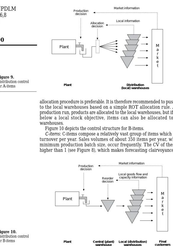
Product availability to the customer is the highest if the inventory is stored close to the customer in the local warehouses as much as possible. It is therefore preferred to use a supply driven (“push”) planning mechanism for the replenishment of the A-items. As soon as the batches are available from production, they are immediately shipped to the local warehouses. Under these circumstances, one handling activity can be avoided. Items are put directly on a truck after production instead of being taken into central storage, and they are immediately shipped to a local warehouse. As production takes place frequently, distribution schedules from plant to local warehouses are also stabilized. To avoid handling inefficiencies, which is necessary owing to product characteristics (low value density, high product volume[17]) and the high volume of the goods flow, products need to be handled in stillage quantities as much as possible. The amount allocated to a local warehouse is determined based on a run out time (ROT) allocation rule. This rule equalizes the expected time until a stockout occurs in the local warehouses (see, for example, Brown[18]). Figure 9 graphically depicts the A-item control framework.
B-items: As opposed to A-items, B-items are characterized by medium sales
volumes with consequently less stable demand (see Figure 9). Products are mature and are produced less frequently than A-items. The production frequency is once a month or less and the size of the CV is larger than with A-items, leading to a relatively higher imbalance risk. Sales of B-items are between 15 and 200 units per week. As opposed to A-items, central stock keeping is thus necessary for B-items. Owing to the imbalance risk, a central and integral overview over stock is necessary. Production is planned based on aggregate forecasts of customer demand. Distribution capacity currently is sufficiently available. The potential savings from better capacity use are therefore small. The potential savings from lower stock are also small owing to the low value of the product. This reduces the need to plan the allocation of goods to the local DCs in a sophisticated way. As a result of this and due to the large number of items and the reduced reliability of local forecasts, a simple
IJPDLM
26,8
90
allocation procedure is preferable. It is therefore recommended to push the items to the local warehouses based on a simple ROT allocation rule. After each production run, products are allocated to the local warehouses, but if stock falls below a local stock objective, items can also be allocated to the local warehouses.
Figure 10 depicts the control structure for B-items.
C-items: C-items compose a relatively vast group of items which have a low
turnover per year. Sales volumes of about 350 items per year, which is the minimum production batch size, occur frequently. The CV of these items is higher than 1 (see Figure 8), which makes forecasting clairvoyance. Frequent
Figure 10. Distribution control for B-items M a r k e t Production decision Market information Reorder decision
Local goods flow and capacity information Plant Plant Final customers Local (distribution) warehouses Central (plant) warehouse Figure 9. Distribution control for A-items Production decision Market information Allocation decision Plant Plant Distribution (local) warehouses Local information M a r k e t
Distribution
control
91
transportation of the items in small batches is not preferable owing to the high transportation costs. As the product value is low, the increase in transportation costs will not outweigh the potential savings in inventory costs. Besides, total capital tied up in C-item inventory is not predominantly determined by the distribution frequency but by the production frequency. Every time a production batch comes available from production, the stock should therefore be pushed to local warehouses, just as with A-items. However, owing to the infrequent production and the high imbalance risk, pushing a complete production batch is not recommendable. Similar to A- and B-items, a ROT rule is proposed for the allocation.
Large batch size to avoid inefficiency in handling are recommendable due to product characteristics (high volume and low value density). To avoid imbalance, only a part of the production batch should be pushed down to the local warehouses. The rest should be retained in a central warehouse. This procedure is known in the literature as the α-policy[19]. In the α-policy, the first batch (100*αper cent of the production batch, with 100*αper cent for example equal to 70 per cent) is pushed through to the local warehouses without storage in the central warehouse. The rest, i.e. (1–α) part of the production batch, is retained in the central warehouse. As soon as one of the local warehouses is running out of inventory, the remaining inventory is allocated to all warehouses. This rest is allocated all at once to enable the use of large batch sizes. Large batch sizes are needed owing to the low value density of the product[15]. In this way, delaying the allocation decision leads to the ability to balance inventory in the distribution system. Figure 11 depicts the control technique.
New items: New items are introduced once a year when the new product
catalogue is published. As soon as the item is available in the catalogue,
Figure 11. Distribution control for C-items M a r k e t Production decision Market information First allocation decision
Local goods flow and capacity information Plant Plant Final customers Local (distribution) warehouses Central (plant) warehouse Second allocation decision 1 – 1 – α α α
IJPDLM
26,8
92
customers tend to request it in rather high quantities to fill up their own distribution system, but the precise moment and amount of this demand peak is unknown. It is therefore important to have stock available in the local warehouses in large quantities. As there is no direct historical demand information available, other sources of information need to be used, such as demand of predecessors and the number of cars for which the exhaust system will be used. Therefore, a co-ordination meeting for demand management is necessary to set up plans and to co-ordinate the allocation of items towards the local warehouses. For the rest, the allocation of goods is similar to that of C-items with both central and decentral stock. Central stock is necessary to be able to rebalance inventory as imbalance risk is high. An α-policy is proposed and distribution batch sizes are relatively large to avoid handling inefficiencies. As opposed to C-items, however, obsolescence risk is relatively small owing to the fact that items are new. The amount of inventory available at local warehouses must therefore be high, as it is important to be able to fill the first customer demand for these new items. Second and later allocations take place as soon as one or more local warehouses are running out of inventory. If enough demand information about an item is available (for example, after one year), the new items can be allocated to one of the other categories. Figure 12 depicts the control technique graphically.
Integration and implementation of control situations
Up to now, we have defined A-, B-, and C- items based on their European demand, implicitly assuming that if an item is a fast mover, it is a fast mover in every market it is sold. It is unrealistic to assume that an exhaust system can be
Figure 12. Distribution control for new items
M a r k e t Production decision Market information Plant Plant Final customers Local (distribution) warehouses Central (plant) warehouse 1 – 1 – α Additional information Co-ordination meeting Local goods flow and capacity information Later allocation decision First allocation decision α α
Distribution
control
93
defined as a fast mover or a slow mover in every market and for every local warehouse. An item may be a fast mover in one market and a medium-fast mover or even a slow mover in another. For example, as there are many French cars in France, exhaust systems for them will be sold in large quantities there. The number of French cars in the UK, on the other hand, is very small, and so, therefore, will be the demand for exhaust systems of French cars. As it is the policy of ESE to produce items as close to their largest market as possible, these items will be produced in France.
In many publications on ABC-analyses, the difference between overall (European) rank and local rank is omitted. It is the combination of the European and the local rank, however, that determines the control technique. As a result, the same item may be controlled differently in different markets. Below, we briefly discuss the combinations of European and local ranks. We omit the new item in this discussion, as new items are new at the same time for all markets.
A-item on European level
For items which are A-items on European level, solutions to resolve the problem of the difference in the European and the local rank are most straightforward. Products are produced every week, so central stock is not necessary. Owing to the relatively high production frequency, all items can be directly shipped from production to the local warehouses via a push system. If the A-item (European level) is a B-, or C-item locally, the shipments from plant to local warehouses need to take place less frequently to maintain relatively large distribution batch sizes for reasons of handling efficiency.
B-item on European level
For B-items, there is central stock. If a European B-item is an A-item in a country, production of this item is assigned to the plant located nearest to that country. In this case, stock is as close to the market as possible. If it is a B-item, stock is allocated each time a production batch is made based on the ROT rule. Between two production runs, the local warehouses can reorder from the central stock based on this ROT rule as well (i.e. reorder if the local stock is below a prespecified number of weeks of demand). The procedure used is therefore a combination of push and pull. For items which are C-items locally, it is first checked whether the C-countries have sufficient inventory until the next production run each time the products are produced. If this is not the case, stock needs to be allocated to these local warehouses. Between two production runs, the inventory retained in the central warehouse for allocating stock to the B-countries can also be used for C-items in case of too low stocks in C-B-countries. However, this needs to be determined centrally. The system used is a hybrid system. Products are pushed to local warehouses after each production run in such a way that it is attempted to cover at least the local demand during two production runs. If stock falls below a preset level between two production runs, stock may be pulled by the C-item countries based on the local stock position.
IJPDLM
26,8
94
C-item on European level
If an item is a C-item on European level, research indicated that it will never be an A-item locally[15]. If it is a B- or a C-item locally, the α-policy is still usable as total demand volumes are still small (it is still a C-item on European level).
Table II summarizes the potential combinations between the level of European demand and of local demand in a distribution control framework.
Conclusions
In this case study, the selection of distribution control techniques in physical distribution has been discussed. A method has been presented, which can be used by a company to select an appropriate distribution control technique. More details about this approach are discussed in the forthcoming dissertation[9].
The conclusions that can be drawn from the case study are summarized below.
ABC classifications are also useful for the selection of control techniques
ABC classifications are predominantly used in inventory control for determining which items should get managerial attention and for parameter setting[2]. This study has shown that this classification can also be a very useful tool for the selection of control techniques in physical distribution systems.
It is recommendable for the selection of appropriate distribution control techniques to define clusters of the products in the assortment
To be able to take account of the specific characteristics of the products distributed, the processes used and the markets served, it is generally not recommended to have only one distribution control technique for all products produced and distributed by a company. A differentiation in distribution control between clusters is therefore desirable. This clustering should be performed in such a way that the characteristics of the products distributed, the process used and markets served within such a cluster, are similar among the members of the cluster and differ between products from different clusters. In the case study discussed, two criteria have been used for the clustering, product sales volume and product life cycle phase, entailing in four different control situations. No process characteristics were used as a clustering criterion, as these characteristics were similar among the products.
Local rank European rank
A-item B-item C-item
A-item Push Push Not applicable
B-item Push Push/pull hybrid α-policy C-item Push Push/pull hybrid α-policy Table II.
Distribution control framework: combinations of European and local ranks
Distribution
control
95
The question whether central stock should be kept is to a large extentdependent on the production frequency
Items with a large demand are produced frequently (once per week). This, combined with the fact that the coefficient of variation of demand is relatively small, leads to the possibility to skip central stock for these items. The items produced are therefore immediately shipped to the local DCs, resulting in a reduction in handling activities. Especially for products with a low value density such as exhaust systems, handling activities are relatively expensive. As a result, the savings are significant for these items.
The ABC classification of an item on European level may differ from its classification on local level
When a classification is used that is based on sales volume, such as the ABC classification, it should be taken into account that the classification of an item on European level may differ from its classification on local level. As a result, an item which is a fast mover on a European level, may be a slow mover at one of the local levels. This difference should be taken into account in the selection of distribution control techniques.
The use of appropriate control techniques may reduce handling costs significantly
For products with a low value density, such as exhaust systems, it is desirable to reduce the handling costs. This can be achieved by minimizing the number of allocations to the local DCs. For A-items, a control technique has been selected in which each production batch is completely allocated to the local DCs without leaving any central stock. However, for items where the stock imbalance risk plays an important role, some central stock is needed. To resolve the problem of stock imbalance while still keeping handling costs relatively low, the production batch should be allocated only partly to the local DCs. Part of the batch should be kept in central stock. This central stock should be allocated to the local DCs completely at the moment there is a need for stock. In this way, only two allocations are needed which keeps handling costs low while stock imbalance is avoided.
Notes and references
1. De Leeuw, S.L.J.M., “A method for designing distribution control systems”, in Platts, K.W., Gregory, M.J. and Neely, A.D. (Eds), Operations Strategy and Performance, Proceedings of
the First European Operations Management Association Conference, University of
Cambridge, Cambridge, 1994, pp. 457-62.
2. Silver, E.A. and Peterson, R., Decision Systems for Inventory Management and Production
Planning, 2nd ed., John Wiley and Sons, New York, NY, 1985.
3. Van Donselaar, K.H., “Material co-ordination under uncertainty”, PhD thesis, Eindhoven University of Technology, The Netherlands, 1989.
4. Martin, A.J., Distribution Resources Planning: the Gateway to True Quick Response and
Continuous Replenishment, 2nd ed., Oliver Wight, Brattleboro, VT, 1993.
IJPDLM
26,8
96
6. Goldratt, E.M. and Cox, J., The Goal (revised ed.), North River Press, Croton-on-Hudson, ONT, 1986.
7. LaLonde, B.J., Masters, J.M., Allenby, G.M. and Maltz, A., “On the adoption of DRP”,
Journal of Business Logistics, Vol. 13 No. 1, 1992, pp. 47-67.
8. De Leeuw, S.L.J.M., “DRP is no castor oil!” (in Dutch: “DRP is geen paardemiddel!”),
Tijdschrift voor Inkoop en Logistiek, Vol. 10 No. 4, 1994, pp.14-18.
9. De Leeuw, S.L.J.M., “The selection of distribution control techniques in a contingency perspective”, PhD dissertation, Eindhoven University of Technology, The Netherlands, 1996 (forthcoming).
10. Van der Linden, P.M.J. and Grunwald, H., “On the choice of a production control system”,
International Journal of Production Research, Vol. 18 No. 2, 1980, pp. 273-9 .
11. Hoekstra, Sj. and Romme, J.H.J.M., Towards Integral Logistic Structures – Developing
Customer Oriented Goods Flows, McGraw-Hill, New York, NY, 1993.
12. Bertrand, J.W.M., Wijngaard, J. and Wortmann, J.C., Production Control: A Structural and
Design Oriented Approach, Elsevier, Amsterdam, The Netherlands, 1990.
13. Meal, H.C., “Putting production decisions where they belong”, Harvard Business Review, March-April, 1984, pp. 102-11.
14. The name of the company has been changed.
15. Van der Snel, K.,“ Distribution control project”, MSc thesis, Eindhoven University of Technology, The Netherlands, 1994.
16. The CV is defined as the standard deviation σdivided by the mean µ; a large value of the CV indicates relatively large variations.
17. Ploos van Amstel, M.J., “Physical distribution strategy and product characteristics”,
International Journal of Physical Distribution and Logistics Management, Vol. 16 No. 1,
1986, pp. 14-36.
18. Brown, R.G., Materials Management Systems, John Wiley & Sons, New York, NY, 1977. 19. Erkip, N.K., A Restricted Class of Allocation Policies in a Two Echelon System, Technical
Report No. 628, School of Operations Research and Industrial Engineering, Cornell University, Ithaca, New York, NY, 1984.