An Introduction to
Partial Least Squares Regression
Randall D. Tobias, SAS Institute Inc., Cary, NC
Abstract
Partial least squares is a popular method for soft modelling in industrial applications. This paper intro-duces the basic concepts and illustrates them with a chemometric example. An appendix describes the experimental PLS procedure of SAS/STATsoftware.
Introduction
Research in science and engineering often involves using controllable and/or easy-to-measure variables
(factors) to explain, regulate, or predict the behavior of
other variables (responses). When the factors are few in number, are not significantly redundant (collinear), and have a well-understood relationship to the re-sponses, then multiple linear regression (MLR) can be a good way to turn data into information. However, if any of these three conditions breaks down, MLR can be inefficient or inappropriate. In such so-called
soft scienceapplications, the researcher is faced with
many variables and ill-understood relationships, and the object is merely to construct a good predictive model. For example, spectrographs are often used
C o m p o n e n t 1 = 0 . 3 7 0 C o m p o n e n t 2 = 0 . 1 5 2 C o m p o n e n t 3 = 0 . 3 3 7 C o m p o n e n t 4 = 0 . 4 9 4 C o m p o n e n t 5 = 0 . 5 9 3
Figure 2: Spectrograph for a mixture
to estimate the amount of different compounds in a chemical sample. (See Figure 2.) In this case, the factors are the measurements that comprise the spec-trum; they can number in the hundreds but are likely to be highly collinear. The responses are component amounts that the researcher wants to predict in future samples.
Partial least squares(PLS) is a method for
construct-ing predictive models when the factors are many and highly collinear. Note that the emphasis is on pre-dicting the responses and not necessarily on trying to understand the underlying relationship between the variables. For example, PLS is not usually appropriate for screening out factors that have a negligible effect on the response. However, when prediction is the goal and there is no practical need to limit the number of measured factors, PLS can be a useful tool. PLS was developed in the 1960’s by Herman Wold as an econometric technique, but some of its most avid proponents (including Wold’s son Svante) are chemical engineers and chemometricians. In addi-tion to spectrometric calibraaddi-tion as discussed above, PLS has been applied to monitoring and controlling industrial processes; a large process can easily have hundreds of controllable variables and dozens of out-puts.
The next section gives a brief overview of how PLS works, relating it to other multivariate techniques such as principal components regression and maximum re-dundancy analysis. An extended chemometric exam-ple is presented that demonstrates how PLS models are evaluated and how their components are inter-preted. A final section discusses alternatives and extensions of PLS. The appendices introduce the ex-perimental PLS procedure for performing partial least squares and related modeling techniques.
How Does PLS Work?
In principle, MLR can be used with very many factors. However, if the number of factors gets too large (for example, greater than the number of observations), you are likely to get a model that fits the sampled data perfectly but that will fail to predict new data well. This phenomenon is calledover-fitting. In such cases, although there are many manifest factors, there may be only a few underlying or latent factors that account for most of the variation in the response. The general idea of PLS is to try to extract these latent factors, accounting for as much of the manifest factor variation
as possible while modeling the responses well. For this reason, the acronym PLS has also been taken to mean ‘‘projection to latent structure.’’ It should be noted, however, that the term ‘‘latent’’ does not have the same technical meaning in the context of PLS as it does for other multivariate techniques. In particular, PLS does not yield consistent estimates of what are called ‘‘latent variables’’ in formal structural equation modelling (Dykstra 1983, 1985).
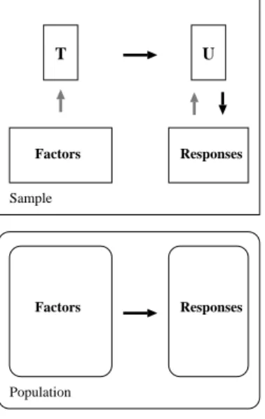
Figure 3 gives a schematic outline of the method. The overall goal (shown in the lower box) is to use
Factors Responses
Population Sample
Factors Responses
T U
Figure 3: Indirect modeling
the factors to predict the responses in the population. This is achieved indirectly by extracting latent vari-ablesT andU from sampled factors and responses,
respectively. The extracted factors T (also referred to as X-scores) are used to predict theY-scores U,
and then the predicted Y-scores are used to construct predictions for the responses. This procedure actu-ally covers various techniques, depending on which source of variation is considered most crucial.
Principal Components Regression (PCR):
The X-scores are chosen to explain as much of the factor variation as possible. This ap-proach yields informative directions in the factor space, but they may not be associated with the shape of the predicted surface.
Maximum Redundancy Analysis (MRA) (van
den Wollenberg 1977): The Y-scores are
cho-sen to explain as much of the predicted Y varia-tion as possible. This approach seeks direcvaria-tions in the factor space that are associated with the most variation in the responses, but the predic-tions may not be very accurate.
Partial Least Squares: The X- and Y-scores
are chosen so that the relationship between
successive pairs of scores is as strong as pos-sible. In principle, this is like a robust form of redundancy analysis, seeking directions in the factor space that are associated with high vari-ation in the responses but biasing them toward directions that are accurately predicted.
Another way to relate the three techniques is to note that PCR is based on the spectral decomposition of
X 0
X, whereX is the matrix of factor values; MRA is
based on the spectral decomposition of ^ Y 0
^
Y, where ^
Y is the matrix of (predicted) response values; and
PLS is based on the singular value decomposition of
X 0
Y. In SASsoftware, both the REG procedure and
SAS/INSIGHTsoftware implement forms of principal components regression; redundancy analysis can be performed using the TRANSREG procedure.
If the number of extracted factors is greater than or equal to the rank of the sample factor space, then PLS is equivalent to MLR. An important feature of the method is that usually a great deal fewer factors are required. The precise number of extracted factors is usually chosen by some heuristic technique based on the amount of residual variation. Another approach is to construct the PLS model for a given number of factors on one set of data and then to test it on another, choosing the number of extracted factors for which the total prediction error is minimized. Alternatively, van der Voet (1994) suggests choosing the least number of extracted factors whose residuals are not significantly greater than those of the model with minimum error. If no convenient test set is available, then each observation can be used in turn as a test set; this is known ascross-validation.
Example:
Spectrometric
Calibra-tion
Suppose you have a chemical process whose yield has five different components. You use an instrument to predict the amounts of these components based on a spectrum. In order to calibrate the instrument, you run 20 different known combinations of the five components through it and observe the spectra. The results are twenty spectra with their associated com-ponent amounts, as in Figure 2.
PLS can be used to construct a linear predictive model for the component amounts based on the spec-trum. Each spectrum is comprised of measurements at 1,000 different frequencies; these are the factor levels, and the responses are the five component amounts. The left-hand side of Table shows the individual and cumulative variation accounted for by
Table 2: PLS analysis of spectral calibration, with cross-validation Number of Percent Variation Accounted For Cross-validation
PLS Factors Responses Comparison
Factors Current Total Current Total PRESS P
0 1.067 0 1 39.35 39.35 28.70 28.70 0.929 0 2 29.93 69.28 25.57 54.27 0.851 0 3 7.94 77.22 21.87 76.14 0.728 0 4 6.40 83.62 6.45 82.59 0.600 0.002 5 2.07 85.69 16.95 99.54 0.312 0.261 6 1.20 86.89 0.38 99.92 0.305 0.428 7 1.15 88.04 0.04 99.96 0.305 0.478 8 1.12 89.16 0.02 99.98 0.306 0.023 9 1.06 90.22 0.01 99.99 0.304 * 10 1.02 91.24 0.01 100.00 0.306 0.091
the first ten PLS factors, for both the factors and the responses. Notice that the first five PLS factors ac-count for almost all of the variation in the responses, with the fifth factor accounting for a sizable proportion. This gives a strong indication that five PLS factors are appropriate for modeling the five component amounts. The cross-validation analysis confirms this: although the model with nine PLS factors achieves the absolute minimum predicted residual sum of squares (PRESS), it is insignificantly better than the model with only five factors.
The PLS factors are computed as certain linear combi-nations of the spectral amplitudes, and the responses are predicted linearly based on these extracted fac-tors. Thus, the final predictive function for each response is also a linear combination of the spectral amplitudes. The trace for the resulting predictor of the first response is plotted in Figure 4. Notice that
Figure 4: PLS predictor coefficients for one response a PLS prediction is not associated with a single fre-quency or even just a few, as would be the case if we tried to choose optimal frequencies for predicting each response (stepwise regression). Instead, PLS prediction is a function of all of the input factors. In
this case, the PLS predictions can be interpreted as contrasts between broad bands of frequencies.
Discussion
As discussed in the introductory section, soft science applications involve so many variables that it is not practical to seek a ‘‘hard’’ model explicitly relating them all. Partial least squares is one solution for such problems, but there are others, including
other factor extraction techniques, like principal
components regression and maximum redun-dancy analysis
ridge regression, a technique that originated
within the field of statistics (Hoerl and Kennard 1970) as a method for handling collinearity in regression
neural networks, which originated with attempts
in computer science and biology to simulate the way animal brains recognize patterns (Haykin 1994, Sarle 1994)
Ridge regression and neural nets are probably the strongest competitors for PLS in terms of flexibility and robustness of the predictive models, but neither of them explicitly incorporates dimension reduction---that is, linearly extracting a relatively few latent factors that are most useful in modeling the response. For more discussion of the pros and cons of soft modeling alternatives, see Frank and Friedman (1993).
There are also modifications and extensions of partial least squares. The SIMPLS algorithm of de Jong
(1993) is a closely related technique. It is exactly the same as PLS when there is only one response and invariably gives very similar results, but it can be dramatically more efficient to compute when there are many factors. Continuum regression(Stone and Brooks 1990) adds a continuous parameter, where
0 1, allowing the modeling method to vary
continuously between MLR ( =0), PLS (=0:5),
and PCR ( = 1). De Jong and Kiers (1992)
de-scribe a related technique calledprincipal covariates
regression.
In any case, PLS has become an established tool in chemometric modeling, primarily because it is often possible to interpret the extracted factors in terms of the underlying physical system---that is, to derive ‘‘hard’’ modeling information from the soft model. More work is needed on applying statistical methods to the selection of the model. The idea of van der Voet (1994) for randomization-based model comparison is a promising advance in this direction.
For Further Reading
PLS is still evolving as a statistical modeling tech-nique, and thus there is no standard text yet that gives it in-depth coverage. Geladi and Kowalski (1986) is a standard reference introducing PLS in chemomet-ric applications. For technical details, see Naes and Martens (1985) and de Jong (1993), as well as the references in the latter.
References
Dijkstra, T. (1983), ‘‘Some comments on maximum likelihood and partial least squares methods,’’ Journal of Econometrics, 22, 67-90.
Dijkstra, T. (1985).Latent variables in linear stochas-tic models: Reflections on maximum likelihood
and partial least squares methods.2nd ed.
Ams-terdam, The Netherlands: Sociometric Research Foundation.
Geladi, P, and Kowalski, B. (1986), ‘‘Partial least-squares regression: A tutorial,’’Analytica
Chim-ica Acta, 185, 1-17.
Frank, I. and Friedman, J. (1993), ‘‘A statistical view of some chemometrics regression tools,’’
Tech-nometrics, 35, 109-135.
Haykin, S. (1994). Neural Networks, a
Comprehen-sive Foundation.New York: Macmillan.
Helland, I. (1988), ‘‘On the structure of partial least squares regression,’’Communications in
Statis-tics, Simulation and Computation, 17(2),
581-607.
Hoerl, A. and Kennard, R. (1970), ‘‘Ridge regression: biased estimation for non-orthogonal problems,’’
Technometrics, 12, 55-67.
de Jong, S. and Kiers, H. (1992), ‘‘Principal covari-ates regression,’’ Chemometrics and Intelligent
Laboratory Systems, 14, 155-164.
de Jong, S. (1993), ‘‘SIMPLS: An alternative approach to partial least squares regression,’’
Chemomet-rics and Intelligent Laboratory Systems, 18,
251-263.
Naes, T. and Martens, H. (1985), ‘‘Comparison of pre-diction methods for multicollinear data,’’ munications in Statistics, Simulation and
Com-putation, 14(3), 545-576.
Ranner, Lindgren, Geladi, and Wold, ‘‘A PLS kernel algorithm for data sets with many variables and fewer objects,’’Journal of Chemometrics, 8, 111-125.
Sarle, W.S. (1994), ‘‘Neural Networks and Statis-tical Models,’’ Proceedings of the Nineteenth Annual SAS Users Group International Confer-ence, Cary, NC: SAS Institute, 1538-1550. Stone, M. and Brooks, R. (1990), ‘‘Continuum
regres-sion: Cross-validated sequentially constructed prediction embracing ordinary least squares, partial least squares, and principal components regression,’’Journal of the Royal Statistical
So-ciety, Series B, 52(2), 237-269.
van den Wollenberg, A.L. (1977), ‘‘Redundancy Analysis--An Alternative to Canonical Correla-tion Analysis,’’Psychometrika, 42, 207-219. van der Voet, H. (1994), ‘‘Comparing the predictive
ac-curacy of models using a simple randomization test,’’ Chemometrics and Intelligent Laboratory
Systems, 25, 313-323.
SAS, SAS/INSIGHT, and SAS/STAT are registered trademarks of SAS Institute Inc. in the USA and other countries.indicates USA registration.
Appendix 1: PROC PLS: An
Exper-imental SAS Procedure for Partial
Least Squares
An experimental SAS/STAT software procedure, PROC PLS, is available with Release 6.11 of the SAS System for performing various factor-extraction methods of modeling, including partial least squares. Other methods currently supported include alternative algorithms for PLS, such as the SIMPLS method of de Jong (1993) and the RLGW method of Rannar et al. (1994), as well as principal components regression. Maximum redundancy analysis will also be included in a future release. Factors can be specified using GLM-type modeling, allowing for polynomial, cross-product, and classification effects. The procedure offers a wide variety of methods for performing cross-validation on the number of factors, with an optional test for the appropriate number of factors. There are output data sets for cross-validation and model information as well as for predicted values and estimated factor scores. You can specify the following statements with the PLS procedure. Items within the brackets<>are optional.
PROC PLS<options>; CLASSclass-variables;
MODELresponses=effects</option>; OUTPUT OUT=SAS-data-set<options>;
PROC PLS Statement
PROC PLS<options>;
You use the PROC PLS statement to invoke the PLS procedure and optionally to indicate the analysis data and method. The following options are available:
DATA =SAS-data-set
specifies the input SAS data set that con-tains the factor and response values.
METHOD =factor-extraction-method
specifies the general factor extraction method to be used. You can specify any one of the following:
METHOD=PLS<(PLS-options)>
specifies partial least squares. This is the default factor extraction method.
METHOD=SIMPLS
specifies the SIMPLS method of de Jong (1993). This is a more effi-cient algorithm than standard PLS; it
is equivalent to standard PLS when there is only one response, and it invariably gives very similar results.
METHOD=PCR
specifies principal components re-gression.
You can specify the followingPLS-options
in parentheses after METHOD=PLS:
ALGORITHM=PLS-algorithm
gives the specific algorithm used to compute PLS factors. Available algo-rithms are
ITER the usual iterative NIPALS al-gorithm
SVD singular value decomposi-tion of X
0
Y, the most exact
but least efficient approach
EIG eigenvalue decomposition of
Y 0
XX
0 Y
RLGW an iterative approach that is efficient when there are many factors
MAXITER=number
gives the maximum number of itera-tions for the ITER and RLGW algo-rithms. The default is 200.
EPSILON=number
gives the convergence criterion for the ITER and RLGW algorithms. The default is 10 12.
CV =cross-validation-method
specifies the cross-validation method to be used. If you do not specify a cross-validation method, the default action is not to perform cross-validation. You can specify any one of the following:
CV = ONE
specifies one-at-a-time cross- valida-tion
CV = SPLIT<(n)>
specifies that every n
th observation
be excluded. You may optionally specify n; the default is 1, which is
the same as CV=ONE.
CV = BLOCK<(n)>
specifies that blocks of n
th
observa-tions be excluded. You may option-ally specifyn; the default is 1, which
CV = RANDOM<(cv-random-opts)>
specifies that random observations be excluded.
CV = TESTSET(SAS-data-set)
specifies a test set of observations to be used for cross-validation.
You also can specify the following
cv-random-opts in parentheses after CV =
RANDOM:
NITER =number
specifies the number of random sub-sets to exclude.
NTEST =number
specifies the number of observations in each random subset chosen for exclusion.
SEED =number
specifies the seed value for random number generation.
CVTEST<(cv-test-options)>
specifies that van der Voet’s (1994) randomization-based model comparison test be performed on each cross-validated model. You also can specify the
follow-ing cv-test-options in parentheses after
CVTEST:
PVAL =number
specifies the cut-off probability for declaring a significant difference. The default is 0.10.
STAT =test-statistic
specifies the test statistic for the model comparison. You can specify either T2, for Hotelling’s T
2 statistic,
or PRESS, for the predicted residual sum of squares. T2 is the default.
NSAMP =number
specifies the number of randomiza-tions to perform. The default is 1000.
LV =number
specifies the number of factors to extract. The default number of factors to extract is the number of input factors, in which case the analysis is equivalent to a regular least squares regression of the responses on the input factors.
OUTMODEL =SAS-data-set
specifies a name for a data set to contain information about the fit model.
OUTCV =SAS-data-set
specifies a name for a data set to contain information about the cross-validation.
CLASS Statement
CLASSclass-variables;
You use the CLASS statement to identify classifica-tion variables, which are factors that separate the observations into groups.
Class-variables can be either numeric or character.
The PLS procedure uses the formatted values of
class-variablesin forming model effects. Any variable
in the model that is not listed in the CLASS statement is assumed to be continuous. Continuous variables must be numeric.
MODEL Statement
MODELresponses=effects</ INTERCEPT>;
You use the MODEL statement to specify the re-sponse variables and the independent effects used to model them. Usually you will just list the names of the independent variables as the model effects, but you can also use the effects notation of PROC GLM to specify polynomial effects and interactions. By default the factors are centered and thus no inter-cept is required in the model, but you can specify the INTERCEPT option to override this behavior.
OUTPUT Statement
OUTPUT OUT=SAS-data-set keyword = names
<:::keyword=names>;
You use the OUTPUT statement to specify a data set to receive quantities that can be computed for every input observation, such as extracted factors and predicted values. The following keywords are available:
PREDICTED predicted values for responses YRESIDUAL residuals for responses XRESIDUAL residuals for factors
XSCORE extracted factors (X-scores, latent vectors,T)
YSCORE extracted responses (Y-scores,U)
STDY standard error for Y predictions STDX standard error for X predictions H approximate measure of influence PRESS predicted residual sum of squares T2 scaled sum of squares of scores
XQRES sum of squares of scaled residuals for factors
YQRES sum of squares of scaled residuals for responses
Appendix 2: Example Code
The data for the spectrometric calibration example is in the form of a SAS data set called SPECTRA with 20 observations, one for each test combination of the five components. The variables are
X1 :::X1000- the spectrum for this combination Y1 :::Y5- the component amounts
There is also a test data set of 20 more observations available for cross-validation. The following state-ments use PROC PLS to analyze the data, using the SIMPLS algorithm and selecting the number of factors with cross-validation.
proc pls data = spectra method = simpls lv = 9 cv = testset(test5) cvtest(stat=press); model y1-y5 = x1-x1000; run;
The listing has two parts (Figure 5), the first part summarizing the cross-validation and the second part showing how much variation is explained by each ex-tracted factor for both the factors and the responses. Note that the extracted factors are labeled ‘‘latent variables’’ in the listing.
The PLS Procedure
Cross Validation for the Number of Latent Variables Test for larger
residuals than minimum Number of Root
Latent Mean Prob > Variables PRESS PRESS ---0 1.0670 0 1 0.9286 0 2 0.8510 0 3 0.7282 0 4 0.6001 0.00500 5 0.3123 0.6140 6 0.3051 0.6140 7 0.3047 0.3530 8 0.3055 0.4270 9 0.3045 1.0000 10 0.3061 0.0700
Minimum Root Mean PRESS = 0.304457 for 9 latent variables Smallest model with p-value > 0.1: 5 latent variables
The PLS Procedure
Percent Variation Accounted For Number of
Latent Model Effects Dependent Variables Variables Current Total Current Total ---1 39.3526 39.3526 28.7022 28.7022 2 29.9369 69.2895 25.5759 54.2780 3 7.9333 77.2228 21.8631 76.1411 4 6.4014 83.6242 6.4502 82.5913 5 2.0679 85.6920 16.9573 99.5486