Multi-Tenant Databases for Software as a Service:
Schema-Mapping Techniques
Stefan Aulbach
†Torsten Grust
†Dean Jacobs
$Alfons Kemper
†Jan Rittinger
††Technische Universität München, Germany $
SAP AG, Walldorf, Germany
{stefan.aulbach,torsten.grust, [email protected]
jan.rittinger,alfons.kemper}@in.tum.de
ABSTRACT
In the implementation of hosted business services, multi-ple tenants are often consolidated into the same database to reduce total cost of ownership. Common practice is to map multiple single-tenant logical schemas in the applica-tion to one multi-tenant physical schema in the database. Such mappings are challenging to create because enterprise applications allow tenants to extend the base schema, e.g., for vertical industries or geographic regions. Assuming the workload stays within bounds, the fundamental limitation on scalability for this approach is the number of tables the database can handle. To get good consolidation, certain ta-bles must be shared among tenants and certain tata-bles must be mapped into fixed generic structures such as Universal and Pivot Tables, which can degrade performance.
This paper describes a new schema-mapping technique for multi-tenancy called Chunk Folding, where the logical ta-bles are vertically partitioned into chunks that are folded to-gether into different physical multi-tenant tables and joined as needed. The database’s “meta-data budget” is divided between application-specific conventional tables and a large fixed set of generic structures called Chunk Tables. Good performance is obtained by mapping the most heavily-uti-lized parts of the logical schemas into the conventional ta-bles and the remaining parts into Chunk Tata-bles that match their structure as closely as possible. We present the re-sults of several experiments designed to measure the efficacy of Chunk Folding and describe the multi-tenant database testbed in which these experiments were performed.
Categories and Subject Descriptors
H.4 [Information Systems Applications]: Miscellaneous; H.2.1 [Information Systems]: Database Management— Logical Design
General Terms
Design, PerformancePermission to make digital or hard copies of all or part of this work for personal or classroom use is granted without fee provided that copies are not made or distributed for profit or commercial advantage and that copies bear this notice and the full citation on the first page. To copy otherwise, to republish, to post on servers or to redistribute to lists, requires prior specific permission and/or a fee.
SIGMOD’08,June 9–12, 2008, Vancouver, BC, Canada. Copyright 2008 ACM 978-1-60558-102-6/08/06 ...$5.00. Add Features Decrease Capital Expenditures Decrease Opera-tional Expenditures
On-Premises Software Software as a Service
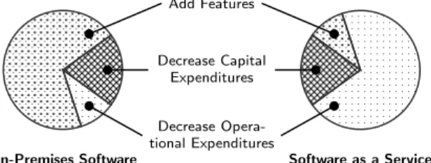
Figure 1: Software Development Priorities
1.
INTRODUCTION
In the traditional on-premises model for software, a busi-ness buys applications and deploys them in a data center that it owns and operates. The Internet has enabled an al-ternative model – Software as a Service (SaaS) – where own-ership and management of applications are outsourced to a service provider. Businesses subscribe to a hosted service and access it remotely using a Web browser and/or Web Service clients. Hosted services have appeared for a wide variety of business applications, including Customer Rela-tionship Management (CRM), Supplier RelaRela-tionship Man-agement (SRM), Human Capital ManMan-agement (HCM), and Business Intelligence (BI). IDC estimates that the worldwide revenue associated with SaaS reached $3.98 billion in 2006 and that it will reach $14.5 billion in 2011, representing a compound annual growth rate (CAGR) of 30% [24].
Design and development priorities for SaaS differ greatly from those for on-premises software, as illustrated in Fig-ure 1. The focus of on-premises software is generally on adding features, often at the expense of reducing total cost of ownership. In contrast, the focus of SaaS is generally on reducing total cost of ownership, often at the expense of adding features. The primary reason for this is, of course, that the service provider rather than the customer has to bear the cost of operating the system. In addition, the re-curring revenue model of SaaS makes it unnecessary to add features in order to drive purchases of upgrades.
A well-designed hosted service reduces total cost of owner-ship by leveraging economy of scale. The greatest improve-ments in this regard are provided by amulti-tenant archi-tecture, where multiple businesses are consolidated onto the same operational system. Multi-tenancy invariably occurs at the database layer of a service; indeed this may be the only place it occurs since application servers for highly-scalable Web applications are often stateless [14].
The amount of consolidation that can be achieved in a multi-tenant database depends on the complexity of the
ap-Email Collaboration CRM/SRM ERP HCM Complexity of Application 10,000 1,000 10,000 100 1,000 10,000 10 100 1,000 Blade Big Iron
Size of Host Machine
Figure 2: Number of Tenants per Database (Solid circles denote existing applications, dashed circles denote estimates)
plication and the size of the host machine, as illustrated in Figure 2. In this context, a tenant denotes an organiza-tion with multiple users, commonly around 10 for a small to mid-sized business. For simple Web applications like busi-ness email, a single blade server can support up to 10,000 tenants. For mid-sized enterprise applications like CRM, a blade server can support 100 tenants while a large cluster database can go up to 10,000. While the total cost of owner-ship of a database may vary greatly, consolidating hundreds of databases into one will save millions of dollars per year.
One downside of multi-tenancy is that it can introduce contention for shared resources [19], which is often alleviated by forbidding long-running operations. Another downside is that it can weaken security, since access control must be per-formed at the application level rather than the infrastructure level. Finally, multi-tenancy makes it harder to support ap-plication extensibility, since shared structures are harder to individually modify. Extensibility is required to build spe-cialized versions of enterprise applications, e.g., for partic-ular vertical industries or geographic regions. Many hosted business services offer platforms for building and sharing such extensions [21, 22, 26].
In general, multi-tenancy becomes less attractive as appli-cation complexity increases. More complex appliappli-cations like Enterprise Resource Planning (ERP) and Financials require more computational resources, as illustrated in Figure 2, have longer-running operations, require more sophisticated extensibility, and maintain more sensitive data. Moreover, businesses generally prefer to maintain more administrative control over such applications, e.g., determining when back-ups, restores, and upgrades occur. More complex applica-tions are of course suitable for single-tenant hosting.
1.1
Implementing Multi-Tenant Databases
In order to implement multi-tenancy, most hosted services use query transformation to map multiple single-tenant log-ical schemas in the application to one multi-tenant physi-cal schema in the database. Assuming the workload stays within bounds, the fundamental limitation on scalability for this approach is the number of tables the database can han-dle, which is itself dependent on the amount of available memory. As an example, IBM DB2 V9.1 [15] allocates 4 KB of memory for each table, so 100,000 tables consume 400 MB of memory up front. In addition, buffer pool pages are allo-cated on a per-table basis so there is great competition for the remaining cache space. As a result, the performance on a blade server begins to degrade beyond about 50,000 tables.
Account
AccountHealthCare
ChunkTable1
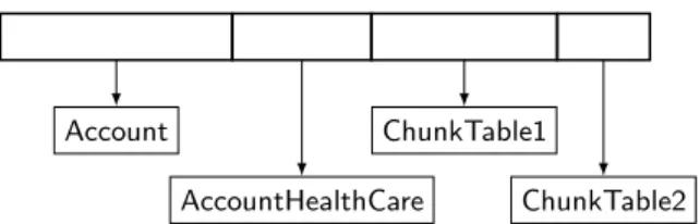
ChunkTable2 Figure 3: Chunk Folding
The natural way to ameliorate this problem is to share tables among tenants. However this technique can interfere with a tenant’s ability to extend the application, as discussed above. The most flexible solution is to map the logical tables into fixed generic structures, such as Universal and Pivot Tables [11]. Such structures allow the creation of an arbi-trary number of tables with arbiarbi-trary shapes and thus do not place limitations on consolidation or extensibility. In addi-tion, they allow the logical schemas to be modified without changing the physical schema, which is important because many databases cannot perform DDL operations while they are on-line. However generic structures can degrade perfor-mance and, if they are not hidden behind the query trans-formation layer, complicate application development.
Our experience is that the mapping techniques used by most hosted services today provide only limited support for extensibility and/or achieve only limited amounts of con-solidation. In particular, simpler services on the left side of Figure 2 tend to favor consolidation while more complex services on the right side tend to favor extensibility.
1.2
Contributions of this Paper
This paper describes a new schema-mapping technique for multi-tenancy called Chunk Folding, where the logical ta-bles are vertically partitioned into chunks that are folded to-gether into different physical multi-tenant tables and joined as needed. The database’s “meta-data budget” is divided between application-specific conventional tables and a large fixed set of generic structures called Chunk Tables. As an example, Figure 3 illustrates a case where the first chunk of a row is stored in a conventional table associated with the base entity Account, the second chunk is stored in a conventional table associated with an extension for health care, and the remaining chunks are stored in differently-shaped Chunk Tables. Because Chunk Folding has a generic component, it does not place limitations on consolidation or extensibility and it allows logical schema changes to occur while the database is on-line. At the same time, and in contrast to generic structures that use only a small, fixed number of tables, Chunk Folding attempts to exploit the database’s entire meta-data budget in as effective a way as possible. Good performance is obtained by mapping the most heavily-utilized parts of the logical schemas into the conventional tables and the remaining parts into Chunk Ta-bles that match their structure as closely as possible.
This paper presents the results of several experiments de-signed to measure the efficacy of Chunk Folding. First, we characterize the performance degradation that results as a standard relational database handles more and more tables. This experiment is based on a multi-tenant database testbed we have developed that simulates a simple hosted CRM ser-vice. The workload contains daily create, read, update, and delete (CRUD) operations, simple reporting tasks, and ad-ministrative operations such as modifying tenant schemas.
The experiment fixes the number of tenants, the amount of data per tenant, and the load on the system, and varies the number of tables into which tenants are consolidated.
Our second experiment studies the performance of stan-dard relational databases on OLTP queries formulated over Chunk Tables. These queries can be large but have a sim-ple, regular structure. We compare a commercial database with an open source database and conclude that, due to dif-ferences in the sophistication of their query optimizers, con-siderably more care has to be taken in generating queries for the latter. The less-sophisticated optimizer complicates the implementation of the query-transformation layer and forces developers to manually inspect plans for queries with new shapes. In any case, with enough care, query optimiz-ers can generate plans for these queries that are efficiently processed. A goal of our on-going work is to compare the penalty of reconstructing rows introduced by Chunk Folding with the penalty for additional paging introduced by man-aging lots of tables.
This paper is organized as follows. To underscore the im-portance of application extensibility, Section 2 presents a case study of a hosted service for project management. Sec-tion 3 outlines some common schema-mapping techniques for multi-tenancy, introduces Chunk Folding, and surveys related work. Section 4 outlines our multi-tenant database testbed. Section 5 describes our experiments with manag-ing many tables. Section 6 describes our experiments with queries over Chunk Tables. Section 7 summarizes the paper and discusses future work.
2.
THE CASE FOR EXTENSIBILITY
Extensibility is clearly essential for core enterprise appli-cations like CRM and ERP. But it can also add tremendous value to simpler business applications, like email and project management, particularly in the collaborative environment of the Web. To underscore this point, this section presents a case study of a hosted business service called Conject [6]. Conject is a collaborative project-management environ-ment designed for the construction and real estate indus-tries. Users of the system include architects, contractors, building owners, and building managers. Participants inter-act inproject workspaces, which contain the data and pro-cesses associated with building projects. Within a project workspace, participants can communicate using email, in-stant messaging, white boards, and desktop sharing. All discussions are archived for reference and to resolve any sub-sequent legal disputes. Documents such as drawings can be uploaded into a project workspace, sorted, selectively shared among participants, and referenced in discussions. Tasks may be defined and assigned to participants and the progress of the project is tracked as tasks are completed. Integrated reports can be issued for the control and documentation of a project. Requests for bids can be created and bids can be submitted, viewed, and accepted.At present, Conject has about 6000 projects shared by 15,000 registered participants across 400 organizations. The system maintains 2 TB of documents in a file-based store and 20 GB of structured data in a commercial database. Data is maintained in conventional, application-specific ta-bles that are shared across projects, participants, and their organizations. A single database instance on a 2.4 GHz dual-core AMD Opteron 250 machine with 8 GB of memory man-ages the full load of 50 million transactions per year.
In the future, Conject will support more sophisticated business processes such as claim management, defect man-agement, issue manman-agement, and decision tracking. Such processes can vary greatly across projects and must be specif-ically designed by the participants. Current plans are to allow participants to associate an object with additional at-tributes, a set of states, and allowable transitions between those states. Participants will be able to save, reuse, and share these configurations. To implement these features, the current fixed database schema will have to be enhanced to support extensibility using techniques such as the ones discussed in this paper.
3.
SCHEMA-MAPPING TECHNIQUES
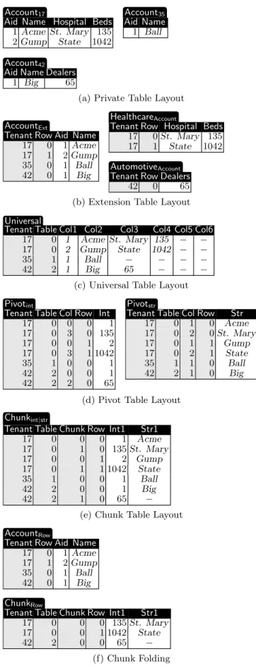
This section outlines some common schema-mapping tech-niques for multi-tenancy, introduces Chunk Folding, and surveys related work. Figure 4 illustrates a running example that shows various layouts for Accounttables of three ten-ants with IDs 17, 35, and 42. Tenant 17 has an extension for the health care industry while tenant 42 has an extension for the automotive industry.
Basic Layout. The most basic technique for implement-ing multi-tenancy is to add a tenant ID column (Tenant) to each table and share tables among tenants. This approach provides very good consolidation but no extensibility. As a result of the latter, it cannot represent the schema of our running example and is not shown in Figure 4. This ap-proach is taken by conventional Web applications, which view the data as being owned by the service provider rather than the individual tenants, and is used by many simpler services on the left side of Figure 2.
Private Table Layout– Figure 4(a). The most basic way to support extensibility is to give each tenant their own pri-vate tables. In this approach, the query-transformation layer needs only to rename tables and is very simple. Since the meta-data is entirely managed by the database, there is no overhead for meta-data in the data itself (the gray columns in Figure 4). However only moderate consolidation is pro-vided since many tables are required. This approach is used by some larger services on the right side of Figure 2 when a small number of tenants can produce sufficient load to fully utilize the host machine.
Extension Table Layout – Figure 4(b). The above two layouts can be combined by splitting off the extensions into separate tables. Because multiple tenants may use the same extensions, the extension tables as well as the base tables should be given aTenantcolumn. ARowcolumn must also be added so the logical source tables can be reconstructed. The two gray columns in Figure 4(b) represent the overhead for meta-data in the data itself.
At run-time, reconstructing the logical source tables car-ries the overhead of additional joins as well as additional I/O if the row fragments are not clustered together. On the other hand, if a query does not reference one of the tables, then there is no need to read it in, which can improve per-formance. This approach provides better consolidation than the Private Table Layout, however the number of tables will still grow in proportion to the number of tenants since more tenants will have a wider variety of basic requirements.
This approach has its origins in the Decomposed Stor-age Model [7], where an n-column table is broken up into n 2-column tables that are joined through surrogate val-ues. This model has then been adopted by column-oriented
Account17
Aid Name Hospital Beds
1Acme St. Mary 135 2Gump State 1042 Account35 Aid Name 1 Ball Account42 Aid Name Dealers
1 Big 65
(a) Private Table Layout
AccountExt
Tenant Row Aid Name
17 0 1Acme
17 1 2Gump
35 0 1 Ball
42 0 1 Big
HealthcareAccount
Tenant Row Hospital Beds
17 0St. Mary 135
17 1 State 1042
AutomotiveAccount Tenant Row Dealers
42 0 65
(b) Extension Table Layout
Universal
Tenant Table Col1 Col2 Col3 Col4 Col5 Col6
17 0 1 Acme St. Mary 135 − −
17 0 2 Gump State 1042 − −
35 1 1 Ball − − − −
42 2 1 Big 65 − − −
(c) Universal Table Layout
Pivotint
Tenant Table Col Row Int
17 0 0 0 1 17 0 3 0 135 17 0 0 1 2 17 0 3 1 1042 35 1 0 0 1 42 2 0 0 1 42 2 2 0 65 Pivotstr
Tenant Table Col Row Str
17 0 1 0 Acme 17 0 2 0St. Mary 17 0 1 1 Gump 17 0 2 1 State 35 1 1 0 Ball 42 2 1 0 Big
(d) Pivot Table Layout
Chunkint|str
Tenant Table Chunk Row Int1 Str1
17 0 0 0 1 Acme 17 0 1 0 135St. Mary 17 0 0 1 2 Gump 17 0 1 1 1042 State 35 1 0 0 1 Ball 42 2 0 0 1 Big 42 2 1 0 65 −
(e) Chunk Table Layout
AccountRow
Tenant Row Aid Name
17 0 1Acme
17 1 2Gump
35 0 1 Ball
42 0 1 Big ChunkRow
Tenant Table Chunk Row Int1 Str1
17 0 0 0 135St. Mary
17 0 0 1 1042 State
42 2 0 0 65 −
(f) Chunk Folding
Figure 4: Account table and its extensions in differ-ent layouts. (Gray columns represdiffer-ent meta-data.)
databases [4, 23], which leverage the ability to selectively read in columns to improve the performance of analytics [23] and RDF data [1]. The Extension Table Layout does not partition tables all the way down to individual columns, but rather leaves them in naturally-occurring groups. This ap-proach has been used to map object-oriented schemas with inheritance into the relational model [9].
Universal Table Layout– Figure 4(c). Generic structures allow the creation of an arbitrary number of tables with ar-bitrary shapes. A Universal Table is a generic structure with aTenantcolumn, aTablecolumn, and a large number of generic data columns. The data columns have a flexi-ble type, such as VARCHAR, into which other types can be converted. Then-th column of each logical source table for each tenant is mapped into then-th data column of the Universal Table. As a result, different tenants can extend the same table in different ways. By keeping all of the values for a row together, this approach obviates the need to recon-struct the logical source tables. However it has the obvious disadvantage that the rows need to be very wide, even for narrow source tables, and the database has to handle many null values. While commercial relational databases handle nullsfairly efficiently, they nevertheless use some additional memory. Perhaps more significantly, fine-grained support for indexing is not possible: either all tenants get an index on a column or none of them do. As a result of these is-sues, additional structures must be added to this approach to make it feasible.
This approach has its origins in the Universal Relation [18], which holds the data for all tables and has every column of every table. The Universal Relation was proposed as a conceptual tool for developing queries and was not intended to be directly implemented. The Universal Table described in this paper is narrower, and thus feasible to implement, because it circumvents typing and uses each physical column to represent multiple logical columns.
There have been extensive studies of the use of generic structures to represent semi-structured data. Florescu et al. [11] describe a variety of relational representations for XML data including Universal and Pivot Tables. Our work uses generic structures to represent irregularities between pieces of schema rather than pieces of data.
Pivot Table Layout – Figure 4(d). A Pivot Table is an alternative generic structure in which each field of each row in a logical source table is given its own row. In addition to Tenant,Table, andRowcolumns as described above, a Pivot Table has aColcolumn that specifies which source field a row represents and a single data-bearing column for the value of that field. The data column can be given a flexible type, such as VARCHAR, into which other types are converted, in which case the Pivot Table becomes a Universal Table for the Decomposed Storage Model. A better approach however, in that it does not circumvent typing, is to have multiple Pivot Tables with different types for the data column. To efficiently support indexing, two Pivot Tables can be created for each type: one with indexes and one without. Each value is placed in exactly one of these tables depending on whether it needs to be indexed.
This approach eliminates the need to handle many null values. However it has more columns of meta-data than actual data and reconstructing an n-column logical source
table requires (n−1) aligning joins along theRowcolumn.
interpret-ing the meta-data than the relatively small number of joins needed in the Extension Table Layout. Of course, like the Decomposed Storage Model, the performance can benefit from selectively reading in a small number of columns.
The Pathfinder query compiler maps XML into relations using Pivot-like Tables [13]. Closer to our work is the re-search on sparse relational data sets, which have thousands of attributes, only a few of which are used by any object. Agrawal et al. [2] compare the performance of Pivot Tables (called vertical tables) and conventional horizontal tables in this context and conclude that the former perform better because they allow columns to be selectively read in. Our use case differs in that the data is partitioned by tenant into well-known dense subsets, which provides both a more challenging baseline for comparison as well as more oppor-tunities for optimization. Beckman et al. [3] also present a technique for handling sparse data sets using a Pivot Table Layout. In comparison to our explicit storage of meta-data columns, they chose an “intrusive” approach which manages the additional runtime operations in the database kernel. Cunningham et al. [8] present an “intrusive” technique for supporting general-purpose pivot and unpivot operations. Chunk Table Layout– Figure 4(e). We propose a third generic structure, called aChunk Table, that is particularly effective when the base data can be partitioned into well-known dense subsets. A Chunk Table is like a Pivot Table except that it has a set of data columns of various types, with and without indexes, and theCol column is replaced by aChunkcolumn. A logical source table is partitioned into groups of columns, each of which is assigned a chunk ID and mapped into an appropriate Chunk Table. In comparison to Pivot Tables, this approach reduces the ratio of stored meta-data to actual meta-data as well as the overhead for reconstructing the logical source tables. In comparison to Universal Tables, this approach provides a well-defined way of adding indexes, breaking up overly-wide columns, and supporting typing. By varying the width of the Chunk Tables, it is possible to find a middle ground between these extremes. On the other hand, this flexibility comes at the price of a more complex query-transformation layer.
Chunk Folding – Figure 4(f). We propose a technique calledChunk Foldingwhere the logical source tables are ver-tically partitioned into chunks that are folded together into different physical multi-tenant tables and joined as needed. The database’s “meta-data budget” is divided between ap-plication-specific conventional tables and a large fixed set of Chunk Tables. For example, Figure 4(f) illustrates a case where base Accounts are stored in a conventional table and all extensions are placed in a single Chunk Table. In contrast to generic structures that use only a small, fixed number of tables, Chunk Folding attempts to exploit the database’s entire meta-data budget in as effective a way as possible. Good performance is obtained by mapping the most heavily-utilized parts of the logical schemas into the conventional ta-bles and the remaining parts into Chunk Tata-bles that match their structure as closely as possible.
A goal of our on-going work is to develop Chunk Fold-ing algorithms that take into account the logical schemas of tenants, the distribution of data within those schemas, and the associated application queries. Because these factors can vary over time, it should be possible to migrate data from one representation to another on-the-fly.
4.
THE MTD TESTBED
This section describes the configurable testbed we have developed for experimenting with multi-tenant database im-plementations. The testbed simulates the OLTP component of a hosted CRM service. Conceptually, users interact with the service through browser and Web Service clients. The testbed does not actually include the associated application servers, rather the testbed clients simulate the behavior of those servers. The application is itself of interest because it characterizes a standard multi-tenant workload and thus could be used as the basis for a multi-tenant database bench-mark.
The testbed is composed of several processes. The System Under Test is a multi-tenant database running on a private host. It can be configured for various schema-mapping lay-outs and usage scenarios. A Worker process engages in mul-tiple client sessions, each of which simulates the activities of a single connection from an application server’s database connection pool. Each session runs in its own thread and gets its own connection to the target database. Multiple Workers are distributed over multiple hosts.
The Controller task assigns actions and tenants to Work-ers. Following the TPC-C benchmark [25], the Controller creates a deck of “action cards” with a particular distribu-tion, shuffles it, and deals cards to the Workers. The Con-troller also randomly selects tenants, with an equal distri-bution, and assigns one to each card. Finally, the Controller collects response times and stores them in a Result Data-base. The timing of an action starts when a Worker sends the first request and ends when it receives the last response.
4.1
Database Layout
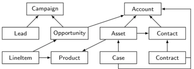
The base schema for the CRM application contains ten tables as depicted in Figure 5. It is a classic DAG-structured OLTP schema with one-to-many relationships from child to parent. Individual users within a business (a tenant) are not modeled, but the same tenant may engage in several simultaneous sessions so data may be concurrently accessed. Every table in the schema has a tenant-id column so that it can be shared by multiple tenants.
Each of the tables contains about 20 columns, one of which is the entity’s ID. Every table has a primary index on the entity ID and a unique compound index on the tenant ID and the entity ID. In addition, there are twelve indexes on selected columns for reporting queries and update tasks. All data for the testbed is synthetically generated.
In order to programmatically increase the overall number of tables without making them too synthetic, multiple copies of the 10-table CRM schema are created. Each copy should be viewed as representing a logically different set of entities. Thus, the more instances of the schema there are in the database, the more schema variability there is for a given amount of data.
In its present form, the testbed models the Extension Ta-ble Layout with many base taTa-bles but no extension taTa-bles. This is sufficient for the experiments on schema variability presented in the next section. The testbed will eventually offer a set of possible extensions for each base table.
4.2
Worker Actions
Worker actions include CRUD operations and reporting tasks that simulate the daily activities of individual users. The reporting tasks model fixed business activity
monitor-LineItem Product Case Contract
Lead Opportunity Asset Contact
Campaign Account
Figure 5: CRM Application Schema
Select Light (50%)Selects all attributes of a single entity or a small set of entities as if they were to be displayed on an entity detail page in the browser.
Select Heavy (15%)Runs one of five reporting queries that perform aggregation and/or parent-child-rollup.
Insert Light (9.59%)Inserts one new entity instance into the data-base as if it had been manually entered into the browser.
Insert Heavy (0.3%) Inserts several hundred entity instances into the database in a batch as if they had been imported via a Web Service interface.
Update Light (17.6%)Updates a single entity or a small set of entities as if they had been modified in an edit page in the browser. The set of entities is specified by a filter condition that relies on a database index.
Update Heavy (7.5%)Updates several hundred entity instances that are selected by the entity ID using the primary key index.
Administrative Tasks (0.01%)Creates a new instance of the 10-table CRM schema by issuing DDL statements.
Figure 6: Worker Action Classes
ing queries, rather than ad-hoc business intelligence queries, and are simple enough to run against an operational OLTP system. Worker actions also include administrative opera-tions for the business as a whole, in particular, adding and deleting tenants. Depending on the configuration, such op-erations may entail executing DDL statements while the sys-tem is on-line, which may result in decreased performance or even deadlocks for some databases. The testbed does not model long-running operations because they should not occur in an OLTP system, particularly one that is multi-tenant.
To facilitate the analysis of experimental results, Worker actions are grouped into classes with particular access char-acteristics and expected response times. Lightweight actions perform simple operations on a single entity or a small set of entities. Heavyweight actions perform more complex opera-tions, such as those involving grouping, sorting, or aggrega-tion, on larger sets of entities. The list of action classes (see Figure 6) specifies the distribution of actions in the Con-troller’s card deck.
The testbed adopts a strategy for transactions that is con-sistent with best practices for highly-scalable Web applica-tions [16, 17]. The testbed assumes that neither browser nor Web Service clients can demarcate transactions and that the maximum granularity for a transaction is therefore the duration of a single user request. Furthermore, since long-running operations are not permitted, large write requests such as cascading deletes are broken up into smaller indepen-dent operations. Any temporary inconsistencies that result from the visibility of intermediate states must be eliminated at the application level. Finally, read requests are always performed with a weak isolation level that permits unre-peatable reads. Schema Variability Number of instances Tenants per instance Total tables 0.0 1 10,000 10 0.5 5,000 2 50,000 0.65 6,500 1 – 2 65,000 0.8 8,000 1 – 2 80,000 1.0 10,000 1 100,000
Table 1: Schema Variability and Data Distribution
5.
HANDLING MANY TABLES
The following section describes an experiment with our multi-tenant database testbed which measures the perfor-mance of a standard relational database as it handles more and more tables. Conventional on-line benchmarks such as TPC-C [25] increase the load on the database until response time goals for various request classes are violated. In the same spirit, our experiment varies the number of tables in the database and measures the response time for various re-quest classes. The testbed is configured with a fixed number of tenants – 10,000 – a fixed amount of data per tenant – about 1.4 MB – and a fixed workload – 40 client sessions. The variable for the experiment is the number of instances of the CRM schema in the database, which we called the schema variability in Section 4.1.
The schema variability takes values from 0 (least variabil-ity) to 1 (most variabilvariabil-ity) as shown in Table 1. For the value 0, there is only one schema instance and it is shared by all tenants, resulting in 10 total tables. At the other ex-treme, the value 1 denotes a setup where all tenants have their own private instance of the schema, resulting in 100,000 tables. Between these two extremes, tenants are distributed as evenly as possible among the schema instances. For ex-ample, with schema variability 0.65, the first 3,500 schema instances have two tenants while the rest have only one.
The experiment was run on a DB2 database server with a 2.8 GHz Intel Xeon processor and 1 GB of memory. The database server was running a recent enterprise-grade Linux operating system. The data was stored on an NFS appli-ance that was connected with dedicated 2 GBit/s Ethernet trunks. The Workers were placed on 20 blade servers with a 1 GBit/s private interconnect.
The experiment was designed in a manner that increas-ing the schema variability beyond 0.5 taxes the ability of the database to keep the primary key index root nodes in memory. Schema variability 0.5 has 50,000 tables, which at 4 KB per table for DB2 consumes about 200 MB of mem-ory. The operating system consumes about 100 MB, leaving about 700 MB for the database buffer pool. The page size for all user data, including indexes, is 8 KB. The root nodes of the 50,000 primary key indexes therefore require 400 MB of buffer pool space. The buffer pool must also accommo-date the actual user data and any additional index pages, and the dataset for a tenant was chosen so that most of the tables need more than one index page.
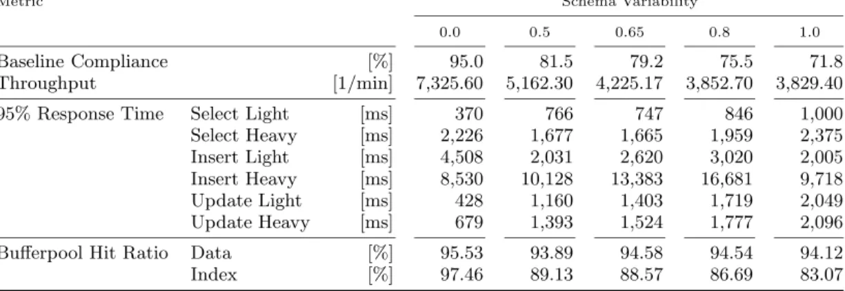
The raw data collected by the Controller was processed as follows. First, the ramp-up phase during which the system reached steady state was stripped off. Then rollups of the results were taken across 30 minute periods for an hour, producing two runs. This process was repeated three times, resulting in a total of six runs. The results of the runs were consistent and so only the first run is reported for each value of the schema variability; see Table 2.
Metric Schema Variability
0.0 0.5 0.65 0.8 1.0
Baseline Compliance [%] 95.0 81.5 79.2 75.5 71.8
Throughput [1/min] 7,325.60 5,162.30 4,225.17 3,852.70 3,829.40
95% Response Time Select Light [ms] 370 766 747 846 1,000
Select Heavy [ms] 2,226 1,677 1,665 1,959 2,375 Insert Light [ms] 4,508 2,031 2,620 3,020 2,005 Insert Heavy [ms] 8,530 10,128 13,383 16,681 9,718
Update Light [ms] 428 1,160 1,403 1,719 2,049
Update Heavy [ms] 679 1,393 1,524 1,777 2,096
Bufferpool Hit Ratio Data [%] 95.53 93.89 94.58 94.54 94.12
Index [%] 97.46 89.13 88.57 86.69 83.07
Table 2: Experimental Results
0 0.5 0.65 0.8 1 50 60 70 80 90 100 Schema Variability Query Percentage
(a) Baseline Compliance
0 0.5 0.65 0.8 1 0 2000 4000 6000 8000 Schema Variability Transactions/Minute (b) Database Throughput 0 0.5 0.65 0.8 1 80 85 90 95 100 Schema Variability Buffer Hit Ratio (%)
Data
Index
(c) Buffer Hit Ratios Figure 7: Results for Various Schema Variability
The first line of this table shows the Baseline Compli-ance, which was computed as follows. The 95% quantiles were computed for each query class of the schema variabil-ity 0.0 configuration: this is the baseline. Then for each configuration, the percentage of queries within the base-line were computed. The lower the basebase-line compliance, the higher the percentage of queries whose response time is above the baseline. Per definition, the baseline compliance of the schema variability 0.0 configuration is 95%. Starting around schema variability 0.65 the high response times are no longer tolerable. The baseline compliance is also depicted in Figure 7(a). The second line of Table 2 is the database throughput in actions per minute, computed as an average over the 30 minute period. The throughput is also depicted in Figure 7(b).
The middle part of Table 2 shows the 95% quantiles for each query class. For the most part, the response times grow with increasing schema variability. We hypothesize that the exceptions occur for the following reasons. First, for low schema variability, there is more sharing among tenants and therefore more contention for longer running queries and tu-ple inserts. Since the heavyweight select queries do aggrega-tion, sorting, or grouping, multiple parallel query instances have impact on each other. The query execution plans show that these queries do a partial table scan with some locking, so the performance for this class degrades. For insert op-erations, the database locks the pages where the tuples are inserted, so concurrently running insert operations have to wait for the release of these locks. This effect can be seen
es-pecially for the lightweight insert operations. Second, there is a visible performance improvement for the insert opera-tions at schema variability 1.0, where the database outper-forms all previous configurations. We hypothesize that this behavior is due to the fact that DB2 is switching between the two insert methods it provides. The first method finds the most suitable page for the new tuple, producing a com-pactly stored relation. The second method just appends the tuple to the end of the last page, producing a sparsely stored relation.
The last two lines of Table 2 show the buffer pool hit ra-tio for the data and the indexes. As the schema variability increases, the hit ratio for indexes decreases while the hit ra-tio for data remains fairly constant. Inspecra-tion of the query plans shows that the queries primarily use the indexes for processing. The hit ratios are also depicted in Figure 7(c).
These experimental results are consistent with anecdotal practical experience using MySQL and the InnoDB storage engine. The hosted email service Zimbra [27] initially exper-imented with a design in which each mailbox was given its own tables [5]. When thousands of mailboxes were loaded on a blade server, performance became unacceptably slow be-cause pages kept getting swapped out of the buffer pool. In addition, when a table is first accessed, InnoDB runs a set of random queries to determine the cardinality of each index, which resulted in a large amount of data flowing through the system. The performance problems disappeared when tables were shared among tenants.
6.
QUERYING CHUNK TABLES
This section describes the transformations needed to pro-duce queries over Chunk Tables by considering the simpler case of Pivot Tables. The generalization to Chunk Tables is straight-forward. This section also discusses the behavior of commercial and open-source databases on those queries.
6.1
Transforming Queries
In the running example of Figure 4, consider the following query from Tenant 17 over the Private Table Layout:
SELECT Beds FROM Account17
WHERE Hospital=‘State’.
(Q1)
The most generic approach to formulating this query over the Pivot Tables Pivotint and Pivotstr is to reconstruct the originalAccount17 table in theFROM clause and then patch it into the selection. Such table reconstruction queries gen-erally consists of multiple equi-joins on the columnRow. In the case ofAccount17, three aligning self-joins on the Pivot table are needed to construct the four-column wide relation. However in Query Q1, the columnsAidandNamedo not ap-pear and evaluation of two of the three mapping joins would be wasted effort.
We therefore devise the following systematic compilation scheme that proceeds in four steps.
1. All table names and their corresponding columns in the logical source query are collected.
2. For each table name, the Chunk Tables and the meta-data identifiers that represent the used columns are obtained.
3. For each table, a query is generated that filters the correct columns (based on the meta-data identifiers from the previous step) and aligns the different chunk relations on theirRowcolumns. The resulting queries are all flat and consist of conjunctive predicates only. 4. Each table reference in the logical source query is
ex-tended by its generatedtable definition query. Query Q1 uses the columns Hospital and Beds of table Account17. The two columns can be found in relationsPivotstr and Pivotint, respectively. For both columns, we know the values of theTenant,Table, andColcolumns. The query to reconstructAccount17checks all these constraints and aligns the two columns on their rows:
(SELECT s.Str as Hospital, i.Int as Beds FROM Pivotstr s, Pivotint i
WHERE s.Tenant = 17 AND i.Tenant = 17
AND s.Table = 0 AND s.Col = 2 AND i.Table = 0 AND i.Col = 3 AND s.Row = i.Row).
(Q1Account17)
To complete the transformation, Query Q1Account17 is then patched into theFROMclause of Query Q1 as a nested sub-query.
When using Chunk Tables instead of Pivot Tables, the re-construction of the logicalAccount17table is nearly identical to the Pivot Table case. In our example, the resultingFROM clause is particularly simple because both requested columns reside in the same chunk (Chunk = 1):
SELECT Beds
FROM (SELECT Str1 as Hospital, Int1 as Beds FROM Chunkint|str WHERE Tenant = 17
AND Table = 0
AND Chunk = 1) AS Account17 WHERE Hospital=‘State’.
(Q1Chunk)
The structural changes to the original query can be sum-marized as follows.
• An additional nesting due to the expansion of the table
definitions is introduced.
• All table references are expanded into join chains on
the base tables to construct the references.
• All base table accesses refer to the columns Tenant, Table,Chunk, and in case of aligning joins, to column Row.
We argue in the following that these changes do not nec-essarily need to affect the query response time.
Additional Nesting. Fegaras and Maier proved in [10] (Rule N8) that the nesting we introduced in theFROMclause – queries with only conjunctive predicates – can always be flattened by a query optimizer. If a query optimizer does not implement such a rewrite (as we will see in Section 6.2) it will first generate the full relation before applying any fil-tering predicates – a clear performance penalty. For such databases, we must directly generate the flattened queries. For more complex queries (with e.g.,GROUP BYclauses) the transformation is however not as clean as the technique de-scribed above.
Join Chains. Replacing the table references by chains of joins on base tables may be beneficial as long as the costs for loading the chunks and applying the index-supported (see below) join are cheaper than reading the wider conventional relations. The observation that different chunks are often stored in the same relation (as in Figure 4(e)) makes this scenario even more likely as the joins would then turn into self-joins and we may benefit from a higher buffer pool hit ratio.
Base Table Access.As all table accesses refer to the meta-data columnsTenant,Table,Chunk, andRowwe should con-struct indexes on these columns. This turns every data ac-cess into an index-supported one. Note that a B-tree index look up in a (Tenant,Table,Chunk,Row) index is basically a partitioned B-tree lookup [12]. The leading B-tree columns (hereTenantandTable) are highly redundant and only par-tition the B-tree into separate smaller B-trees (parpar-titions). Prefix compression makes sure that these indexes stay small despite the redundant values.
6.2
Evaluating Queries
To assess the query performance of standard databases on queries over Chunk Tables, we devised a simple experiment that compares a conventional layout with equivalent Chunk Table layouts of various widths. The first part of this section will describe the schema and the query we used, the second part outlines the experiments we conducted.
Test Schema.The schema for the conventional layout con-sists of two tablesParentandChild:
Parent
id col1 col2 . . . col90 Child
id parent col1 col2 . . . col90
(Conventional)
Both tables have anidcolumn and 90 data columns that are evenly distributed between the typesINTEGER,DATE, and VARCHAR(100). In addition, table Child has a foreign key reference toParentin columnparent.
The Chunk Table layouts each have two tables: ChunkData storing the grouped data columns andChunkIndexstoring the key id and foreign key parent columns of the conventional tables. In the different Chunk Table layouts, theChunkData table varied in width from 3 data columns (resulting in 30 groups) to 90 data columns (resulting in a single group) in 3 column increments. Each set of three columns had types INTEGER,DATE, andVARCHAR(100)allowing groups from the conventional table to be tightly packed into the Chunk Ta-ble. In general, the packing may not be this tight and a Chunk Table may have nulls, although not as many as a Universal Table. TheChunkIndex table always had a single INTEGERcolumn.
As an example, Chunk6 shows a Chunk Table instance of width 6 where each row of a conventional table is split into 15 rows inChunkData and 1 (for parents) or 2 (for children) rows inChunkIndex.
ChunkData
table chunk row int1 int2 date1 date2 str1 str2 ChunkIndex
table chunk row int1
(Chunk6)
For the conventional tables, we created indexes on the primary keys (id) and the foreign key (parent,id) in theChild table. For the chunked tables, we created (table,chunk,row) indexes on all tables (see previous section for the reasons) as well as an (int1,table,chunk,row) index onChunkIndexto mimic the foreign key index on theChildtable.
The tests used synthetically generated data for the in-dividual schema layouts. For the conventional layout, the Parent table was loaded with 10,000 tuples and the Child table was loaded with 100 tuples per parent (1,000,000 tu-ples in total). The Chunk Table Layouts were loaded with equivalent data in fragmented form.
Test Query. Our experiments used the following simple selection query.
SELECT p.id, ... FROM parent p, child c WHERE p.id = c.parent
AND p.id = ?.
(Q2)
Query Q2 has two parameters: (a) the ellipsis (...) rep-resenting a selection of data columns and (b) the question mark (?) representing a random parent id. Parameter (b) ensures that a test run touches different parts of the data. Parameter (a) – theQ2 scale factor – specifies the width of the result. As an example, Query Q23 is Query Q2 with a scale factor of 3: the ellipsis is replaced by 3 data columns
1 2 3 4 5 ChunkIndex ChunkIndex ChunkData
ChunkData ChunkData
ChunkData itcr itcr tcr tcr IXSCAN IXSCAN IXSCAN FETCH IXSCAN FETCH HSJOIN NLJOIN NLJOIN RETURN
Figure 8: Join plan for simple fragment query each for parent and child.
SELECT p.id, p.col1, p.col2, p.col3, c.col1, c.col2, c.col3 FROM parent p, child c WHERE p.id = c.parent
AND p.id = ?.
(Q23)
Higher Q2 scale factors (ranging up to 90) are more chal-lenging for the chunked representation because they require more aligning joins.
Test 1 (Transformation and Nesting). In our first test, we transformed Query Q2 using the methods described in Section 6.1 and fed the resulting queries into the open-source database MySQL [20] and the commercial database DB2. We then used the database debug/explain facilities to look at the compiled query plans. The MySQL optimizer was un-able to unnest the nesting introduced by our query transfor-mation. DB2 on the other hand presented a totally unnested plan where the selective predicate onp.idwas even pushed into the chunk representing the foreign key of the child re-lation. DB2’s evaluation plan is discussed in more detail in the next test.
We then flattened the queries in advance and studied whether the predicate order on the SQL level would influ-ence the query evaluation time. We produced an ordering where all predicates on the meta-data columns preceded the predicates of the original query and compared it with the ordering that mimics DB2’s evaluation plan. For MySQL, the latter ordering outperformed the former ordering by a factor of 5.
After adjusting the query transformation to produce flat-tened queries with predicates in the correct order, we reran the experiment on both databases. DB2 produced the same execution plan and MySQL was able to produce a plan that started with the most selective predicate (p.id = ?). As one would expect, the query evaluation times for MySQL showed an improvement.
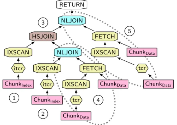
Test 2 (Transformation and Scaling). To understand how queries on Chunk Tables behave with an increasing number of columns (output columns as well as columns used in predicates) we analyzed the plans for a number of queries. The pattern is similar for most queries and we will discuss the characteristics based on Query Q23, which was designed for the Chunk Table Layout in Chunk6.
The query plan is shown in Figure 8. The leaf operators all access base tables. If the base tables are accessed via
Q2 scale factor ((# of data columns)/2 in Q2’sSELECTclause) (ms) 0 6 12 18 24 30 36 42 48 54 60 66 72 78 84 90 0 5 10 15 20 25 30 35 40 45 50 55 N◦ H △• 2 N◦ H △• 2 N ◦ H △• 2 N ◦ H △• 2 N ◦ H △• 2 N ◦ H △• 2 N ◦ H △• 2 N ◦ H △• 2 N ◦ H △• 2 N ◦ H △• 2 N ◦ H △• 2 N ◦ H △ • 2 N ◦ H △ • 2 N ◦ H △ • 2 N ◦ H △ • 2 N ◦ H △ • 2 N ◦ H △ • 2 N ◦ H △ • 2 N ◦ H △ • 2 N ◦ H △ • 2 N ◦ H △ • 2 N ◦ H △ • 2 N ◦ H △ • 2 N ◦ H △ • 2 N ◦ H △ • 2 N ◦ H △ • 2 N ◦ H △ • 2 N ◦ H △ • 2 N ◦ H △ • 2 N ◦ H △ • 2 N ◦ H △ • 2 Chunk Table width:N 3
(# columns) ◦ 6
H15 △30
•90
conventional table: 2
Figure 9: Response Times with Warm Cache an index, anIXSCANoperator sits on top of the base table with a node in between that refers to the used index. Here, the meta-data index is calledtcr(abbreviating the columns table,chunk, androw) and the value index is calleditcr. If a base table access cannot be completely answered by an index (e.g., if data columns are accessed) an additional FETCH operator (with a link to the base table) is added to the plan. Figure 8 contains two different join operators: a hash join (HSJOIN) and an index nested-loop join (NLJOIN).
The plan in Figure 8 can be grouped into 5 regions. In region 1, the foreign key for the child relation is looked up.
The index access furthermore applies the aforementioned selection on the ?parameter. In region 2, the id column of the parent relation is accessed and the same selection as for the foreign key is applied. The hash join in region
3 implements the foreign key join p.id = c.parent. But before this value-based join is applied in region 4, all data
columns for the parent table are looked up. Note that region
4 expands to a chain of aligning joins where the join column row is looked up using the meta-data index tcr if parent columns in different chunks are accessed in the query. A similar join chain is built for the columns of the child table in region 5.
Test 3 (Response Times with Warm Cache). Figure 9 shows the average execution timeswith warm cacheson DB2 V9, with the same database server setup described in Sec-tion 5. We conducted 10 runs; for all of them, we used the same values for parameter?so the data was in memory. In this setting, the overhead compared to conventional tables is entirely due to computing the aligning joins. The queries based on narrow chunks have to perform up to 60 more joins (layout Chunk3with Q2 scale factor 90) than the queries on the conventional tables which results in a 35 ms slower re-sponse time. Another important observation is that already for 15-column wide chunks, the response time is cut in half in comparison to 3-column wide chunks and is at most 10 ms slower than conventional tables.
Test 4 (Logical Page Reads). Figure 10 shows the num-ber of logical data and index page reads requested when executing Query Q2. For all chunked representations, 74% to 80% of the reads were issued by index accesses. Figure 10
Q2 scale factor ((# of data columns)/2 in Q2’sSELECTclause) # logical page reads
0 6 12 18 24 30 36 42 48 54 60 66 72 78 84 90 0 1.000 2.000 3.000 4.000 5.000 6.000 7.000 8.000 9.000 10.000 11.000 12.000 13.000 14.000 15.000 16.000 N◦ H △• 2 N◦ H △ • 2 N ◦ H △ • 2 N ◦ H △ • 2 N ◦ H △ • 2 N ◦ H △ • 2 N ◦ H △ • 2 N ◦ H △ • 2 N ◦ H △ • 2 N ◦ H △• 2 N ◦ H △ • 2 N ◦ H △ • 2 N ◦ H △ • 2 N ◦ H △ • 2 N ◦ H △ • 2 N ◦ H △ • 2 N ◦ H △ • 2 N ◦ H △ • 2 N ◦ H △ • 2 N ◦ H △ • 2 N ◦ H △ • 2 N ◦ H △ • 2 N ◦ H △ • 2 N ◦ H △ • 2 N ◦ H △ • 2 N ◦ H △ • 2 N ◦ H △ • 2 N ◦ H △ • 2 N ◦ H △ • 2 N ◦ H △ • 2 N ◦ H △ • 2 15.950 8.336 3.766 2.243 1.126 215 Chunk Table width:N 3
(# columns) ◦ 6
H15 △30
•90
conventional table: 2
Figure 10: Number of logical page reads.
Q2 scale factor ((# of data columns)/2 in Q2’sSELECTclause) (s) 0 6 12 18 24 30 36 42 48 54 60 66 72 78 84 90 0 1 2 3 4 5 6 7 8 9 10 11 12 13 14 15 N ◦ H △ • 2 N ◦ H △ • 2 N ◦ H △ • 2 N ◦ H △ • 2 N ◦ H △ • 2 N ◦ H △ • 2 N ◦ H △ • 2 N ◦ H △ • 2 N ◦ H △ • 2 N ◦ H △ • 2 N ◦ H △ • 2 N ◦ H △ • 2 N ◦ H △ • 2 N ◦ H △ • 2 N ◦ H △ • 2 N ◦ H △ • 2 N ◦ H △ • 2 N◦ H △ • 2 N◦ H △ • 2 N ◦ H △ • 2 N ◦ H △ • 2 N ◦ H △ • 2 N ◦ H △ • 2 N ◦ H △ • 2 N ◦ H △ • 2 N ◦ H △ • 2 N ◦ H △ • 2 N ◦ H △ • 2 N ◦ H △ • 2 N◦ H △ • 2 Chunk Table width:N 3
(# columns) ◦ 6
H15 △30
•90
conventional table: 2
Figure 11: Response Times with Cold Cache clearly shows that every join with an additional base table increases the number of logical page reads. Thus this graph shows the trade-off between conventional tables, where most meta-data is interpreted at compile time, and Chunk Tables, where the meta-data must be interpreted at runtime. Test 5 (Response Times with Cold Cache). Figure 11 shows the average execution times with cold caches. For this test, the database buffer pool and the disk cache were flushed between every run. For wider Chunk Tables, i.e. 15 to 90 colums, the response times look similar to the page read graph (Figure 10). For narrower Chunk Tables, cache locality starts to have an effect. For example, a single phys-ical page access reads in 2 90 column-wide tuples and 26 6 column-wide tuples. Thus the response times for the nar-rower Chunk Tables are lower than for some of the wider Chunk Tables. For a realistic application, the response times would fall between the cold cache case and the warm cache case.
Test 6 (Cache Locality Benefits). The effects of cache locality are further clarified in Figure 12, which shows the
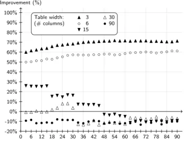
Q2 scale factor ((# of data columns)/2 in Q2’sSELECTclause) Improvement (%) 0 6 12 18 24 30 36 42 48 54 60 66 72 78 84 90 -20% -10% 0% 10% 20% 30% 40% 50% 60% 70% 80% 90% 100% N ◦ H △ • N ◦ H △ • N ◦ H △ • N ◦ H △ • N ◦ H △ • N ◦ H △ • N ◦ H △ • N ◦ H △ • N ◦ H △ • N ◦ H △ • N ◦ H △• N ◦ H △• N ◦ H △• N ◦ H △• N ◦ H △• N ◦ H △ • N ◦ H △• N ◦ H △• N ◦ H △ • N ◦ H △• N ◦ H △ • N ◦ H △ • N ◦ H △ • N ◦ H △ • N ◦ H △ • N ◦ H △ • N ◦ H △ • N ◦ H △ • N ◦ H △ • N ◦ H △ • Table width: N 3 △30 (# columns) ◦ 6 •90 H15
Figure 12: Response Time Improvements for Chunk Tables Compared to Vertical Partitioning
relative difference in response times between Chunk Fold-ing and more conventional vertical partitionFold-ing. In the lat-ter case, the source tables are partitioned as before, but the chunks are kept in separate tables rather than being folded into the same tables. For configurations with 3 and 6 columns, Chunk Folding exhibits a response time improve-ment of more than 50 percent. In the configuration with 90 columns, Chunk Folding and vertical partitioning have nearly identical physical layouts. The only difference is that Chunk Folding has an additional columnChunkto identify the chunk for realigning the rows, whereas in the vertical partitioning case, this identification is done via the physical table name. Since theChunkcolumn is part of the primary index in the Chunk Folding case, there is overhead for fetch-ing this column into the index buffer pools. This overhead produces up to 25% more physical data reads and a response time degradation of 10%.
Additional Tests. We also ran some initial experiments on more complex queries (such as grouping queries). In this case, queries on the narrowest chunks could be as much as an order of magnitude slower than queries on the conventional tables, with queries on the wider chunks filling the range in between.
The overall result of these experiments is that very nar-row Chunk Tables, such as Pivot Tables, carry considerable overhead for reconstruction of rows. As Chunk Tables get wider however, the performance improves considerably and becomes competitive with conventional tables well before the width of the Universal Table is reached.
6.3
Transforming Statements
Section 6.1 presented a systematic compilation scheme for generating queries over Chunk Tables. This section briefly describes how to cope with UPDATE, DELETE, and INSERT statements.
In SQL, data manipulation operations are restricted to single tables or updateable selections/views which the SQL query compiler can break into separate DML statements. For update and delete statements, predicates can filter the tuples affected by the manipulation. As insert and delete
operations also require the modification of meta-data val-ues, we devised a consistent DML query transformation logic based on single table manipulations.
Since multiple chunked tables are required for a single source table, a single source DML statement generally has to be mapped into multiple statements over Chunk Tables. Following common practice, we transform delete operations into updates that mark the tuples as invisible instead of physically deleting them, in order to provide mechanisms like a Trashcan. Such an update naturally has to mark all chunk tables as deleted in comparison to normal updates that only have to manipulate the chunks where at least one cell is affected.
Our DML transformation logic for updates (and thus also for deletes) divides the manipulation into two phases: (a) a query phase that collects all rows that are affected by an update and (b) an update phase that applies the update for each affected chunk with local conditions on the meta-data columns and especially column row only. Phase (a) transforms the incoming query with the query transforma-tion scheme from Sectransforma-tion 6.1 into a query that collects the set of affectedrowvalues. One possibility to implement the updates in Phase (b) is to nest the transformed query from Phase (a) into a nested sub-query using an INpredicate on column row. This approach lets the database execute all the work. For updates with multiple affected chunks (e.g., deletes) the database however has to evaluate the query from Phase (a) for each chunk relation. An alternative approach would be to first evaluate the transformed predicate query, let the application then buffer the result and issue an atomic update for each resulted row value and every affected Chunk Table.
We turn now to insert statements. For any insert, the application logic has to look up all related chunks, collect the meta-data for tables and chunks, and assign each inserted new row a unique row identifier. With the complete set of meta-data in hand, an insert statement for any chunk can be issued.
Other operations like DROP or ALTER statements can be evaluated on-line as well. They however require no access to the database. Instead only the application logic has to do the respective bookkeeping.
6.4
Chunk Tables vs. Chunk Folding
Chunk Folding mixes Extension and Chunk Tables. The inclusion of Extension Tables does not affect the query part of the previous section at all. The reason is that the only interface between the different tables is the meta-column Row, which is also available in the Extension Table Layout. The only important change necessary to make Chunk Fold-ing work is a refinement of the transformation logic in the second bullet of Section 6.1 that enables also the meta-data lookup for Extension Tables.
7.
CONCLUSION
This paper has presentedChunk Folding, a new schema-mapping technique for implementing multi-tenancy on top of a standard relational database. In this technique, the logical tables are vertically partitioned into chunks that are folded together into application-specific conventional tables and a fixed set of generic Chunk Tables. Chunk Tables can vary in width, from very narrow Pivot-like Tables to very wide Universal Tables.
This paper presented the results of several experiments de-signed to measure the efficacy of Chunk Folding. We studied the performance of standard relational databases on OLTP queries formulated over Chunk Tables. Very narrow Chunk Tables can carry considerable overhead for reconstruction of rows, but wider Chunk Tables become competitive in per-formance with conventional tables well before the width of the Universal Table is reached.
Finally, this paper described a multi-tenant database test-bed that simulates a simple hosted CRM service. We used this testbed to characterize the performance degradation that results as a standard relational database handles more and more tables. A goal of our on-going work is to com-pare the penalty of reconstructing rows introduced by Chunk Folding with the penalty for additional paging introduced by managing lots of tables.
More generally, our on-going work entails enhancing the testbed to include extension tables as well as base tables. This framework will allow us to study Chunk Folding in a more complete setting. In particular, our goal is to develop algorithms that take into account the logical schemas of ten-ants, the distribution of data within those schemas, and the associated application queries, and then create a suitable Chunk Table Layout. Because these factors can vary over time, it should be possible to migrate data from one repre-sentation to another on-the-fly.
8.
REFERENCES
[1] D. J. Abadi, A. Marcus, S. Madden, and K. J. Hollenbach. Scalable Semantic Web Data Management Using Vertical Partitioning. InProceedings of the 33rd International Conference on Very Large Data Bases, University of Vienna, Austria, September 23-27, 2007, pages 411–422, 2007.
[2] R. Agrawal, A. Somani, and Y. Xu. Storage and Querying of E-Commerce Data. InVLDB ’01: Proceedings of the 27th International Conference on Very Large Data Bases, pages 149–158, San Francisco, CA, USA, 2001. Morgan Kaufmann Publishers Inc. [3] J. L. Beckmann, A. Halverson, R. Krishnamurthy, and
J. F. Naughton. Extending RDBMSs To Support Sparse Datasets Using An Interpreted Attribute Storage Format. InICDE ’06: Proceedings of the 22nd International Conference on Data Engineering (ICDE’06), page 58, Washington, DC, USA, 2006. IEEE Computer Society.
[4] P. A. Boncz.Monet: A Next-Generation DBMS Kernel For Query-Intensive Applications. Ph.D. Thesis, Universiteit van Amsterdam, Amsterdam, The Netherlands, May 2002.
[5] B. Burtin and S. Dietzen (Zimbra Inc., Sunnyvale, CA, USA). Personal communication, 2007. [6] conject.com.http://www.conject.com/. [7] G. P. Copeland and S. N. Khoshafian. A
decomposition storage model. InSIGMOD ’85: Proceedings of the 1985 ACM SIGMOD international conference on Management of data, pages 268–279, New York, NY, USA, 1985. ACM.
[8] C. Cunningham, G. Graefe, and C. A. Galindo-Legaria. PIVOT and UNPIVOT:
Optimization and Execution Strategies in an RDBMS. In(e)Proceedings of the Thirtieth International
Conference on Very Large Data Bases, Toronto, Canada, August 31 - September 3 2004, pages 998–1009, 2004.
[9] R. Elmasri and S. B. Navathe.Fundamentals of Database Systems, 5th Edition. Addison-Wesley, 2007. [10] L. Fegaras and D. Maier. Optimizing object queries
using an effective calculus.ACM Transactions on Database Systems (TODS), 25(4), 2000.
[11] D. Florescu and D. Kossmann. A Performance Evaluation of Alternative Mapping Schemes for Storing XML Data in a Relational Database. Technical report, Inria, France, 1999.
[12] G. Graefe. Sorting and Indexing with Partitioned B-Trees. InProc. of the 1st Int’l Conference on Innovative Data Systems Research (CIDR), Asilomar, CA, USA, Jan. 2003.
[13] T. Grust, M. V. Keulen, and J. Teubner. Accelerating XPath evaluation in any RDBMS.ACM Trans. Database Syst., 29(1):91–131, 2004.
[14] J. R. Hamilton. On designing and deploying internet-scale services. InProceedings of the 21th Large Installation System Administration Conference, LISA 2007, Dallas, Texas, USA, November 11-16, 2007, pages 231–242. USENIX, 2007.
[15] ibm.com.http://www.ibm.com/.
[16] D. Jacobs. Data management in application servers. In Readings in Database Systems, 4th edition. The MIT Press, 2005.
[17] A. Kemper, D. Kossmann, and F. Matthes. SAP R/3: a database application system (Tutorial). InSIGMOD 1998, Proceedings ACM SIGMOD International Conference on Management of Data, June 2-4, 1998, Seattle, Washington, USA., page 499, 1998.
[18] D. Maier and J. D. Ullman. Maximal objects and the semantics of universal relation databases. ACM Trans. Database Syst., 8(1):1–14, 1983.
[19] Anatomy of MySQL on the GRID.
http://blog.mediatemple.net/weblog/2007/01/19/ anatomy-of-mysql-on-the-grid/.
[20] mysql.com.http://www.mysql.com/.
[21] NetSuite NetFlex.http://www.netsuite.com/ portal/products/netflex/main.shtml. [22] Salesforce AppExchange.
http://www.salesforce.com/appexchange/about. [23] M. Stonebraker, D. J. Abadi, A. Batkin, X. Chen,
M. Cherniack, M. Ferreira, E. Lau, A. Lin, S. Madden, E. J. O’Neil, P. E. O’Neil, A. Rasin, N. Tran, and S. B. Zdonik. C-Store: A Column-oriented DBMS. In Proceedings of the 31st International Conference on Very Large Data Bases, Trondheim, Norway, August 30 - September 2, 2005, pages 553–564, 2005. [24] E. TenWolde. Worldwide Software on Demand
2007-2011 Forecast: A Preliminary Look at Delivery Model Performance, IDC No. 206240, 2007. IDC Report.
[25] TPC-C on-line transaction processing benchmark. http://www.tpc.org/tpcc/.
[26] WebEx.http://www.webex.com/. [27] Zimbra.http://www.zimbra.com/.