Virginia Commonwealth University
VCU Scholars Compass
Theses and Dissertations Graduate School
2014
Spatial Scheduling Algorithms for Production
Planning Problems
Sudharshana Srinivasan
Virginia Commonwealth UniversityFollow this and additional works at:http://scholarscompass.vcu.edu/etd Part of theApplied Mathematics Commons
© The Author
This Dissertation is brought to you for free and open access by the Graduate School at VCU Scholars Compass. It has been accepted for inclusion in Theses and Dissertations by an authorized administrator of VCU Scholars Compass. For more information, please [email protected]. Downloaded from
c
Sudharshana Srinivasan, May 2014
SPATIAL SCHEDULING ALGORITHMS FOR PRODUCTION PLANNING PROBLEMS
A Dissertation submitted in partial fulfillment of the requirements for the degree of Doctor of Philosophy at Virginia Commonwealth University.
by
SUDHARSHANA SRINIVASAN Master of Science in Applied Mathematics Virginia Commonwealth University, May 2011
Director: Dr. J. Paul Brooks,
Associate Professor, Department of Statistics and Operations Research
Virginia Commonwewalth University Richmond, Virginia
In loving memory of Amma. You are, and will always remain, my hero.
Acknowledgements
I embarked upon an educational journey five years ago, without the faintest idea on how to arrive at my destination. I was fortunate to meet the right people at the right time in the right places, who gave me the right direction. This work would not have been possible without the support and assistance provided by these wonderful individuals and I would like to take this opportunity to express my sincerest gratitude to them. Listing every person that showed me the way would fill volumes. Hence I will mention a chosen few and leave the rest in a special place in my heart.
First and foremost, I want to thank my advisors, who have been instrumental in the successful completion of my defense and dissertation. Dr. Jill Wilson, has been a role model for me ever since I started graduate school. She got me interested in operations research and specifically in the exciting area of scheduling. She has always been supportive not only academically, but also emotionally through the rough road to finish this thesis. Dr. Paul Brooks helped me find my dissertation topic and guided me as I inched toward the finish line. I consider myself extremely lucky to have been counseled by these two very remarkable professors. Their expert and valuable insights have made me pursue approaches that I might not have otherwise considered and their careful reading of this document helped me refine my work and its presentation. I would like to thank the members of my doctoral committee, Dr. David Edwards, Dr. Jose Dula, and Dr. Yongjia Song, for taking an interest in evaluating my work and for their time and contribution in helping me finish this last part of my dissertation. I also want to extend my gratitude to Dr. Jason Merrick for having faith in my ability to undertake and complete the doctoral program and for being a constant source of encouragement throughout these years in graduate school. I wish to express my appreciation to Dr. D’Arcy Mays for being the most approachable and cheerful
administrator I have known.
The support and advice from peers and friends made taking classes and tests less of an ordeal. I owe my gratitude to my fellow students, Toni, Ben, Phil, and Derrick, for making this ride memorable. To my ‘lab mates’, Shaun, Robert, Jacob, Eric, and Chris, thank you guys, you officially made friday mornings more enjoyable and productive.
Words are insufficient to convey the emotions I experience when I think of my families. I am forever obliged to the Sorrels, Toni, Calvin, and little Ben, for adopting me and for being my home away from home. I cannot imagine having survived thus far without them. My heartfelt thanks to Aai and Baba, your unconditional love and support provided much needed motivation. I am truly blessed to have become a part of such a lovely family. Finally, a great big hug and thank you to the two most important men in my life - Appa and Advait. Appa you have always believed in me and have given me the freedom to write my own story. Thank you for tolerating my teenage years, for teaching me to be independent, and for being the coolest dad on the planet. Advait, thanks for being amazing, for being there for me when it matters, and for your infinite patience. Your love and encouragement has helped me sail through all the good times and the bouts of frustration, for that I will be eternally indebted.
TABLE OF CONTENTS
Chapter Page
Acknowledgements . . . ii
Table of Contents . . . iv
List of Tables . . . v
List of Figures . . . vii
Abstract . . . ix 1 Introduction . . . 1 1.1 Motivation . . . 1 1.2 Problem Description . . . 4 1.3 Fundamental Concepts . . . 5 1.3.1 Integer programming . . . 5 1.3.2 Computational Complexity . . . 7 1.3.3 Approximation Algorithms . . . 7
2 Spatial Scheduling Problem . . . 9
2.1 Introduction . . . 9
2.2 Background . . . 10
2.3 Formulation . . . 13
2.3.1 Time-indexed Formulation . . . 14
2.3.2 General Mixed-Integer Programming Formulation . . . 15
2.4 Special Cases . . . 16
2.5 Methodology . . . 17
3 Batch-scheduling . . . 19
3.1 Introduction . . . 19
3.1.1 Forming the Batches . . . 23
3.1.1.1 Iterative model . . . 24
3.1.1.2 Efficient Area model . . . 26
3.1.2 Scheduling the batches . . . 28
3.2 Performance Analysis . . . 30
3.3 Computational Analysis . . . 34
3.3.1 Instance Generation . . . 34
3.3.2 Valid Values for T . . . 35
3.3.3 Initial feasible solution heuristic . . . 36
3.3.4 Computational Results . . . 38
4 List-scheduling approach . . . 42
4.1 Introduction . . . 43
4.2 Generating the schedule . . . 44
4.3 Performance Analysis . . . 46
4.4 Upper bounds . . . 49
4.5 Computational Results . . . 49
5 Conclusions . . . 53
Appendix A Batch-scheduling heuristic performance . . . 56
Appendix B List-scheduling heuristic performance . . . 60
References . . . 62
LIST OF TABLES
Table Page
1 Sample instance of the spatial scheduling problem . . . 9
2 Example instance with three jobs such that only jobs 1 and 3
simul-taneously fit the space. . . 20
3 SSP instance with N=6 jobs to depict that grouping more jobs in a
batch does not guarantee lower objective value . . . 33
4 Problem size comparisons between M1, M2, and original SSP MIP
models for N job instances . . . 36
5 Comparison of objectives obtained from M1, M2, and OPT for small
instances of batch-scheduling . . . 39
6 Comparison of M1, M2, and OPT runtimes for small instances of
batch-scheduling . . . 39
7 Comparison of objectives obtained from M1, M2, and ZIP for large
instances of batch-scheduling . . . 40
8 Comparison of M1, M2, andZIP runtimes for large instances of
batch-scheduling . . . 40
9 An example to motivate the need for list-scheduling by area and
pro-cessing time . . . 42
10 Comparing the objective values obtained from greedy heuristic,
list-scheduling product version, and ZIP for instances of SSP . . . 50
11 Comparing runtimes for greedy heuristic, list-scheduling algorithm,
and ZIP while solving instances of SSP . . . 51
12 Comparison of objective values obtained using M1 and M2 with ZIP
13 Comparison of objective values obtained using M1 and M2 with ZIP
for SSP instances with 5 jobs . . . 57
14 Runtimes in seconds for M1, M2, andZIP when solving SSP instances
with 5 jobs . . . 58
15 Runtimes in seconds for M1, M2, andZIP when solving SSP instances
with 10 jobs . . . 59
16 Comparison of objective values obtained using greedy heuristic and
product version of list-scheduling algorithm withZIP for SSP instances
with 5 jobs . . . 60
17 Comparison of objective values obtained using greedy heuristic and
product version of list-scheduling algorithm withZIP for SSP instances
LIST OF FIGURES
Figure Page
1 Depicting the motivation for spatial scheduling with jobs each
requir-ing two time units scheduled over a two-day horizon . . . 11
2 Batching sequence for example with three jobs . . . 20
3 Sequence in which batches are scheduled for Proposition1 . . . 21
4 Comparing strategies for sequencing batches . . . 22
5 Example schedule with two and three jobs in a batch . . . 33
6 List-scheduling algorithm attempts to find the same four contiguous width and three contiguous height units for two consecutive time slots . . 44
Abstract
SPATIAL SCHEDULING ALGORITHMS FOR PRODUCTION PLANNING PROBLEMS
By Sudharshana Srinivasan
A Dissertation submitted in partial fulfillment of the requirements for the degree of Doctor of Philosophy at Virginia Commonwealth University.
Virginia Commonwealth University, 2014.
Director: Dr. J. Paul Brooks,
Associate Professor, Department of Statistics and Operations Research
Spatial resource allocation is an important consideration in shipbuilding and large-scale manufacturing industries. Spatial scheduling problems (SSP) involve the non-overlapping arrangement of jobs within a limited physical workspace such that some scheduling objective is optimized. Since jobs are heavy and occupy large areas, they cannot be moved once set up, requiring that the same contiguous units of space be assigned throughout the duration of their processing time. This adds an addi-tional level of complexity to the general scheduling problem, due to which solving large instances of the problem becomes computationally intractable. The aim of this study is to gain a deeper understanding of the relationship between the spatial and temporal components of the problem. We exploit these acquired insights on problem characteristics to aid in devising solution procedures that perform well in practice. Much of the literature on SSP focuses on the objective of minimizing the makespan of the schedule. We concentrate our efforts towards the minimum sum of comple-tion times objective and state several interesting results encountered in the pursuit
of developing fast and reliable solution methods for this problem. Specifically, we de-velop mixed-integer programming models that identify groups of jobs (batches) that can be scheduled simultaneously. We identify scenarios where batching is useful and ones where batching jobs provides a solution with a worse objective function value. We present computational analysis on large instances and prove an approximation factor on the performance of this method, under certain conditions. We also provide greedy and list-scheduling heuristics for the problem and compare their objectives with the optimal solution. Based on the instances we tested for both batching and list-scheduling approaches, our assessment is that scheduling jobs similar in processing times within the same space yields good solutions. If processing times are sufficiently different, then grouping jobs together, although seemingly makes a more effective use of the space, does not necessarily result in a lower sum of completion times.
CHAPTER 1
INTRODUCTION
1.1 Motivation
Everyday we are confronted by the logistical challenges in planning and alloca-tion of resources (human, material, or a physical quantity) to tasks; examples include the scheduling of processors to jobs in a computing environment, effectively allocating personnel to a project, generating timetables for a school, creating airline schedules, and reserving operating rooms for surgeries. Traditional scheduling problems create schedules that efficiently utilize resources to complete tasks while minimizing some objective criterion. The objective functions encountered in scheduling literature can be broadly classified into min-sum or min-max objectives. For example, minimizing the makespan and minimizing maximum lateness are min-max objectives, while mini-mizing the (weighted) sum of completion or start times of jobs is a min-sum objective. The problems are classified using the three-field classification scheme introduced by Graham et al. 1979, which specifies the machine environment, job characteristics, and optimality criterion for the problem. Further variations to the problems are created by including or excluding, one or more, of the following characteristics:
1. Online scheduling: Job characteristics are known as and when jobs become available.
2. Precedence of jobs: A job cannot be processed until certain other jobs have completed.
4. Due-dates and release-dates: Jobs can be processed only after they are released and have to be processed prior to their due dates. Sometimes tardy jobs are permitted, but penalized.
5. Additional resources: Renewable resources are limited within each time period and replenished at the end of the time period. Equipment and labor are some of the classic examples for renewable resources. Nonrenewable resources, such as capital budget, are limited over the overall planning horizon, but not restricted within each time period.
There are many results on the complexity of these problems under different conditions (Garey, Johnson, and Sethi 1976; Lenstra, Rinnooy Kan, and Brucker 1977). The com-plexity in solving these problems and diversity in their applications have given rise to varied solution methodologies (Baker 1974; Coffman Jr 1976; Pinedo 2008; Lawler et al. 1993; Brucker 2001). While some approaches are exact, others are designed to provide fast, cheap, and reliable solutions. Various general integer programming formulations have been proposed for discrete scheduling problems (Queyranne and Schulz 1994; Dyer and Wolsey 1990). One of the notable exact methods used to solve these mathematical models is the branch and bound method (Land and Doig 1960). Essentially, branch and bound algorithms use lower and upper bounds on the optimal objective value to control the enumeration of its solutions. Often such procedures be-come computationally intractable with an increase in problem size. Hence, there is a need to develop alternative methods that produce near-optimal solutions in poly-nomial time. Approximation algorithms (AA) deliver solutions with provable quality that are bounded in runtime. Heuristics, in contrast, generate quick solutions without any provable performance guarantees.
In the past 50 years, there has been a great deal of work on developing AA for NP hard optimization problems, specifically scheduling problems (Hochbaum 1997; Vazirani 2001). Encouraged by this successful application of AA to scheduling prob-lems (Lee and Chen 2009; Savelsbergh, Uma, and Wein 1998; Hall et al. 1997), this thesis aims to construct approximation algorithms for the spatial scheduling problem with the objective to minimize the sum of completion times. Spatial scheduling prob-lems involve the assignment of a spatial resource along with conventional temporal attributes. Therefore, the solutions should not only specify starting times for each job, but also locations for the placement of jobs on a physical workspace. The mo-tivation for the choice of our objective is two-fold. First, within the realm of spatial scheduling problems, much energy is devoted to studying methods for minimizing the ‘makespan’ or total project duration (Perng, Lai, and Ho 2009; Zheng et al. 2011; Koh et al. 2011; Zhang and Chen 2012; Caprace et al. 2013). Results for other ob-jectives are scarce (Garcia and Rabadi 2011; Kolisch 2000) and to the best of our knowledge this is the first study to consider the sum of completion times objective. Second, when jobs are independent and competing for the same resource, the cost associated with individual completion times becomes more relevant and natural (Le-ung, Kelly, and Anderson 2004). For example, inventory systems may require that certain products with higher overheads per time be processed ahead of others.
The process of designing AA is similar to that of exact algorithms. In order to design reliable algorithms with good performance guarantees, we need to gain an understanding of the structure of the problem. Therefore we concentrate our efforts in examining the simplest form of the problem by considering a workspace area of fixed dimensions. We disallow precedence constraints, due-dates, rotation of jobs, and set-up times. By doing so, we are able to focus on the relationship between the spatial and
temporal components in the problem and gain a better understanding of the problem characteristics. The insights acquired by studying the simple problem can enable us to devise algorithms that perform well in practice. The remainder of this section briefly describes the spatial scheduling problem, provides relevant background, and reviews the fundamental concepts used in subsequent chapters of this dissertation. 1.2 Problem Description
In large-scale production and manufacturing industries, the assembly line in-volves scheduling jobs that each require a certain amount of two-dimensional space within a limited physical workspace. This requires that the schedule not only assign starting times to each job, but also locations and orientations. It is also important to ensure that jobs are assigned the same contiguous units of space throughout the duration of their processing. Thus, any solution to this problem attempts to answers the following questions:
(a) When to schedule the jobs? (Temporal component) (b) Where to schedule the jobs? (Spatial component)
Mathematically, the spatial scheduling problem is described as follows: Given a
setJ of jobs with fixed processing times pj, height hj, and width wj for each j ∈ J
and a workspace B of height H and width W; does there exist a schedule of the
jobs that minimizes the given objective criterion such that the spatial and temporal restrictions in each time period are satisfied? While the spatial restrictions ensure that jobs collectively fit within the physical workspace, the temporal constraints in-volve conditions (if present) on the starting times of the jobs. Common objectives include minimizing total project duration (min-max objective) or minimizing the av-erage time to complete individual jobs (min-sum objective). The number of tasks,
nature of the resources (renewable or non-renewable), and constraints (precedence of tasks, due-dates, or limitations on availability) add to the complexity of the schedul-ing problem.
Throughout the remainder of this thesis we study the spatial scheduling problem
for the objective of minimizing the sum of completion times (denoted by Z). We
disallow precedence constraints, due-dates, rotation of jobs, and set-up times. We will hereafter refer to this variation of the problem as SSP.
1.3 Fundamental Concepts
In this section we present relevant background information on the concepts used in the subsequent chapters of this dissertation. The information presented here can be found in Garey and Johnson 1979, Nemhauser and Wolsey 1988, Vazirani 2001, and Williamson and Shmoys 2010. In what follows, we denote linear programming or linear program as LP, integer programming or integer program as IP, and mixed-integer programming or mixed-mixed-integer program as MIP.
1.3.1 Integer programming
Mathematical programming is a modeling technique that assists in making deci-sions to address real-world problems. The decideci-sions are modeled as unknown variables and the objective, a function of the decision variables, represents the best possible so-lution for the model. The restrictions on decisions being made express the constraints
or mathematical inequalities of the problem. Given a vector c∈Rn andb ∈
Rm, and
a matrix A∈Rmxn, we want to find a vectorx∈
Zn that solves the following integer
mincTx
s.t.Ax≥b
x∈Zn
Relaxing the integrality constraints produces an LP. MIPs use a combination of integer and real-valued variables. The integrality constraints help capture the discrete nature of certain decisions. Both linear and integer programs seek to find an optimal assignment of values to the variables that satisfy the constraints while minimizing or maximizing a linear objective function. LPs are solved using the simplex method (Dantzig 1965) or barrier methods (Karmarkar 1984) and the approach to solving (mixed) integer programs is with the use of branch and bound algorithms, first intro-duced by Land and Doig 1960. The algorithm performs controlled enumeration of the solution space with the use of lower and upper bounds on the optimal solution. The first step is to remove the integrality constraints in the original problem, resulting in an LP relaxation of the problem. Upon solving the relaxation, if we obtain integral solutions, without explicitly imposing them, we have obtained an optimal solution. If not, as is usually the case, we partition the set of integer solutions into two disjoint sets. This is referred to as a variable dichotomy branching strategy. For example, if
an integer variable, say x, has a value of 5.6 in the relaxation, we partition the set of
variables into two sets: one with x ≥ 6 and x ≤ 5. The two new problems created
by branching on variablex are solved and the optimal solution for the problem is the
better solution among the two subproblems. We continue the process of enumeration as we build a search tree by selecting different branching variables. The algorithm terminates when all the subproblems are solved or fathomed. Although the
subprob-lems we are attempting to solve are LPs, using the branch and bound algorithm can take long due to the sheer number of subproblems being solved. One of the ways to optimize the procedure and speed up the process is by using upper bounding (for minimization problems) heuristics or approximation algorithms.
1.3.2 Computational Complexity
Computational complexity theory classifies decision problems based on the in-herent difficulty in solving them computationally. Class P contains problems with instances that can be solved and verified in polynomial time. In other words, the worst-case running-time for these algorithms is polynomial in size of the input. Some-times we may not have an efficient (polynomial time) algorithm for a problem, however if given a solution we may be able to verify its accuracy in polynomial time. These problems are defined as non-deterministic polynomial-time (NP) problems. A
prob-lem p is said to be NP-complete if is it in NP and if every other problem in NP is
reducible to p. Many combinatorial optimization problems have been shown to be
NP-complete by reductions from known NP-complete problems (Garey and Johnson 1979). Approximation and parameterization techniques are commonly used to find reasonable solutions for such problems.
1.3.3 Approximation Algorithms
Although Johnson 1974 coined the term “approximation algorithm”, earlier
papers had proved the performance guarantees of heuristics (Graham 1966). Ap-proximation algorithms deliver solutions with provable quality that are bounded in runtime. Suppose we wish to solve an NP-hard minimization problem consisting of
instances in I. Let z(I)=min{cIx : x ∈ SI} ∀I ∈ I. Let A be an algorithm that
application ofA to I. Let ρ≥1.
Definition 1 A is a ρ-approximation algorithm for I if for each I ∈ I, A runs in time polynomial in the size ofI, and A(I) ≤ρz(I). A is said to have a factorρ, also referred to as the performance guarantee of A.
Observe that we compare the objective value obtained by the application of the
algorithm to instance I with the optimal objective value z(I) for that instance. In
practice, however, this is not possible, because if z(I) is known then there would be
no need to approximate it. To overcome this issue and calculateρ, we compare A(I)
with a lower bound for z(I), say L(I). Lower bounds can be obtained using LP or
combinatorial relaxations. SinceL(I)≤z(I) we have, A(I)≤ρL(I) =⇒ A(I)≤ρz(I).
CHAPTER 2
SPATIAL SCHEDULING PROBLEM
In this chapter we describe the spatial scheduling problem and present mathematical formulations for SSP. We also survey the literature and present our approaches in developing solution methodologies for the problem.
2.1 Introduction
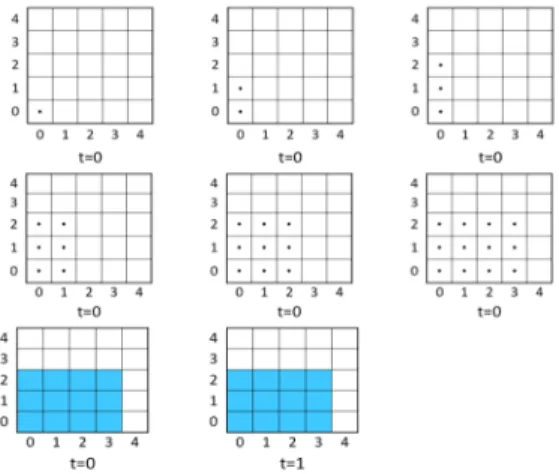
Spatial scheduling is often an important consideration in large-scale manufactur-ing and production industries. Assembly units are often heavy, occupy large areas, and cannot be relocated easily. Therefore they require a fixed quantity of physical space throughout the duration of processing time. Since workspace area available at such facilities is limited, assembly lines need to consider efficient utilization of spa-tial resources along with temporal considerations common to traditional scheduling problems. For example, if we have a workspace of 25 square units, and three jobs with characteristics as specified in Table 1, we would like to find starting times and a layout of the jobs within the given space that minimizes the sum of the completion times objective.
Table 1. Sample instance of the spatial scheduling problem
Job Width Height Processing Time 1 2 1 2
2 2 2 2 3 4 3 2
2.2 Background
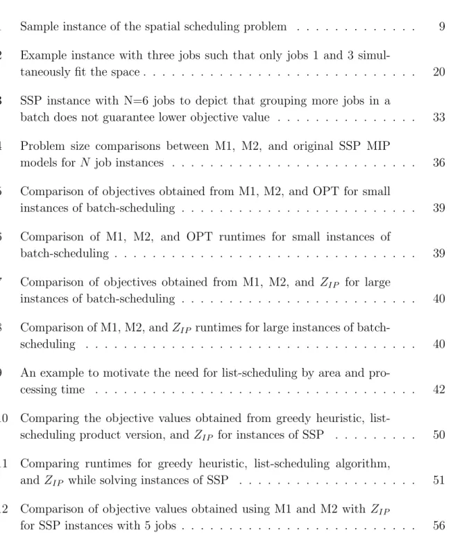
Spatial scheduling problems have been studied in recent years, mostly in the context of shipbuilding (Lee et al. 1997; Park et al. 1996; Cho et al. 2001; Raj and Srivastava 2007). Modern day ship building practices use prefabricated sections or ‘blocks’. These super-structures that occupy large spaces are built elsewhere in the yard and then transported to the building dock for assembly. This is known as ‘block construction’. The shipbuilding facilities usually have a limitation of the space they can provide. Hence they require an optimal method of spacing the assemblies and the equipment required. There are also temporal restrictions such as deadlines and due-dates. Thus, this problem is ideal for spatial scheduling. Figure 1 shows the layout of jobs before and after applying spatial scheduling solution procedures. We can see that initially the space is not utilized effectively and some jobs are waiting to be processed. On applying some spatial scheduling method, we get a better utilization of the space and no delays in processing of jobs.
Pioneering work in this area began between 1991 and 1993, when the Daewoo Shipbuilding Company and Korea Advanced Institute of Science and Technology jointly initiated the DAewoo Shipbuilding Scheduling (DAS) project to develop
in-novative scheduling systems that improve productivity and efficiency. Lee et al.
1997 applied the two-dimensional arrangement of convex polygons at the Daewoo
shipyard. Park et al. 1996 extended this work and applied it at the block painting
shop in the Hyundai shipyard. Cho et al. 2001 included failure blocks, the blocks
that are scheduled but are not worked upon and workload balancing constraints that guaranteed an even distribution of workload on the equipment available. The solu-tion system for the block painting process includes an operasolu-tion strategy algorithm, a block-scheduling algorithm, a block arrangement algorithm, and a block assignment
Fig. 1. Depicting the motivation for spatial scheduling with jobs each requiring two time units scheduled over a two-day horizon
algorithm. Garcia 2010 considers a class of spatial scheduling problems that involve scheduling each job into one of several possible processing areas in parallel to mini-mize total tardiness. The authors suggest an integer programming formulation and a
strip-packing based heuristic to solve the problem. Raj and Srivastava 2007 give a
mixed-integer programming model to describe the spatial scheduling problem. They make assumptions about the orientations of the blocks and use three-dimensional bin-packing approaches to analyze data collected from an Indian shipyard. They also discuss applications of stacking goods in shelves in large retail stores.
Mullen and Butler 2000 present the design of a spatially constrained harvest-scheduling model that uses a genetic algorithm as the optimization technique. A single unit of a forest area containing relatively uniform species composition is re-ferred to as a stand. The genetic algorithm specifies the order by which to place
stands in the schedule by evaluating the population of permutations of the stand identification numbers. Spatial goals are becoming more frequent aspects of forest management plans with changes in regulatory and organizational policies. Enhanc-ing these operations will benefit a variety of economic and conservation objectives. Boston and Bettinger 2001 discuss the addition of green-up constraints, that is, har-vesting restrictions that prevent the cutting of adjacent units for a specified period of time, suggesting the application of spatial schedules to forest plans. The authors discuss a two-stage method that in one stage uses linear programming to assign vol-ume goals, and in a second stage uses a tabu search genetic algorithm technique to minimize the deviations from the volume goals while maximizing the present net
rev-enue. BoWang and Gadow 2002 present a multi-objective function consisting of a
timber component and a spatial component. The model is solved using the method of simulated annealing. It is shown that adjusting the adjacency matrix for the stands generates a variety of spatial harvesting patterns.
Much of the literature focuses on approaches with the objective of minimizing
the makespan or maxj∈JCj, whereCj denotes the completion time of job j in a given
schedule (Perng, Lai, and Ho 2009; Zheng et al. 2011; Koh et al. 2011; Zhang and Chen 2012; Caprace et al. 2013). Garcia and Rabadi 2011 provide a meta heuristic algorithm to minimize the total tardiness for instances with release dates and multiple processing areas. Kolisch 2000 develops a MIP-formulation and list-scheduling algo-rithm that minimizes the weighted sum of tardiness for assembly scheduling problems in the presence of part availability constraints and a spatial resource. While the ap-plications listed above are by no means comprehensive, they demonstrate the value in investigating this problem. The remainder of this document discusses the approaches taken in the pursuit of finding reliable and efficient solution methods for SSP.
2.3 Formulation
In this study, we consider SSP which involves scheduling a setJ of jobs to
mini-mize the sum of completion times (Z) such that the jobs fit within the limited physical
workspaceB of height H and widthW. Each job j ∈J requires a space of heighthj
and widthwj over its processing time pj. Without loss of generality we assume that
the problem data is integer-valued.
In the presentation that follows, we describe two mathematical formulations of SSP; a time-indexed formulation and a general MIP formulation. Time-indexed for-mulations are known to serve as good guides for developing approximation algorithms as they provide strong lower bounds for LP relaxations of scheduling problems (Akker, Van Hoesel, and Savelsbergh 1999; Phillips, Stein, and Wein 1998; Savelsbergh, Uma, and Wein 1998; Goemans 1997; Hall et al. 1997; Sousa and Wolsey 1992). The disad-vantage of using these formulations are their size; even small instances have a large number of variables and constraints (Akker, Hurkens, and Savelsbergh 2000). Al-though decomposition techniques and other cut generation schemes may be used to alleviate some of the computational difficulties encountered (Akker, Hurkens, and Savelsbergh 2000; Lee and Sherali 1994) while implementing these formulations, since our goal is to find solutions quickly we chose the alternate formulation. Note that both formulations presented here minimize the sum of starting times. The sum of
completion times objective used in our analysis ZOP T is then obtained by adding
P
2.3.1 Time-indexed Formulation
The following time-indexed formulation is based on the one provided in Hardin, Nemhauser, and Savelsbergh 2008. Our motivation in creating this formulation is to analyze the polyhedral structure of the problem and potentially identify valid inequalities for the problem.
minX j∈J X t∈T X x∈X X y∈Y rxytj (2.1) subject to: X j∈J qxytj≤1 ∀x∈X, y∈Y, t∈T (2.2) X t∈T X x∈X X yinY rxytj= 1 ∀j∈J (2.3) x+wj−1 X x0=x qx0ytj ≥wjrxytj ∀x∈X, y∈Y, t∈T, j∈J (2.4) y+hj−1 X y0=y qxy0tj ≥hjrxytj ∀x∈X, y∈Y, t∈T, j∈J (2.5) t+pj−1 X t0=t qxyt0j ≥pjrxytj ∀x∈X, y∈Y, t∈T, j∈J (2.6) rxytj, qxytj∈ {0,1} ∀x∈X, y∈Y, t∈T, j ∈J (2.7) where,
J is the set of all jobs
T is the set of all the discretized units of time when a job can be scheduled
X is the set of all possible x-coordinate points that discretize the width of the
workspace
Y is the set of all possible y-coordinate points that discretize the height of the
rxytj =
1 if job j starts at time t at location (x,y) 0 otherwise qxytj=
1 if job j is processing at time t at location (x,y) 0 otherwise
Forx∈X, y∈Y, t∈T, and j ∈J
ZOP T is obtained by adding
P
j∈Jpj to the objective in (2.1). Constraint (2.2)
en-sures that there is only be one job that is processing at any given time and location and constraint (2.3) guarantees that each job starts exactly once. The constraints (2.4-2.6) relate the starting time of the jobs with the time periods that the job is
processing. If a job j starts at time t at location (x, y), then it must be processing
until time period t+pj −1 at locations x tox+wj −1 andy to y+hj−1.
2.3.2 General Mixed-Integer Programming Formulation
The following mixed-integer programming formulation based on two dimensional bin packing problem has been adapted from Garcia 2010.
minX j∈J zj (2.8) subject to: −xi+xj−W αij ≥ −W +wi ∀i, j∈J, i6=j (2.9) −yi+yj −Hβij ≥ −H+hi ∀i, j∈J, i6=j (2.10) −zi+zj−T γij ≥ −T+pi ∀i, j∈J, i6=j (2.11) αij+αji+βij +βji+γij+γji ≥1 ∀i, j∈J, i6=j (2.12) −xi−wi≥ −W ∀i∈J (2.13) −yi−hi ≥ −H ∀i∈J (2.14) xi, yi, zi ≥0 ∀i∈J (2.15) αij, βij, γij ∈ {0,1} ∀i, j∈J (2.16) where,
J is the set of all jobs
xj is the x-coordinate of job j ∈J
yj is the y-coordinate of job j ∈J
zj is the z-coordinate (start time) for job j ∈J
αij =
1 if no overlap occurs between jobs i and j in the x direction 0 otherwise βij =
1 if no overlap occurs between jobs i and j in y direction 0 otherwise γij =
1 if no overlap occurs between jobs i and j in z direction 0 otherwise
For i, j ∈J
Here, T is an upper bound on the makespan of the schedule. ZOP T is obtained by
addingP
j∈Jpj to the objective in (2.8). Constraints (2.9)-(2.12) prevent overlap from
occurring in the x (width), y (height), and z (time) dimensions. We use constraints (2.13) and (2.14) to ensure that the jobs are confined to the physical dimensions of the workspace.
2.4 Special Cases
The original motivation for studying SSP was to better understand the relation-ships between the spatial and temporal components of the problem. The following special cases of SSP have interesting applications and we anticipate that some of our results can aid in developing solution methods for these problems or vice-versa.
1. Bin Packing
Given a set J of items, the bin packing problem attempts to find the minimum
contained in exactly one bin. In an instance of SSP if we normalize processing
times and widths of jobs such that pj = 1 andwj = 1, ∀j ∈J and W = 1, then
solutions to SSP can be viewed as solutions to the bin packing problem, where
bins of size H correspond to the the time periods in the schedule and items of
size hj,∀j ∈J correspond to the jobs.
2. Single Machine Scheduling
Instances of SSP with wj = W and hj = H, ∀ jobs j ∈ J reduce to instances
of single machine scheduling problems, where jobs consume all of the available spatial resource during each time period that its processing.
3. Uniform Resource-Constrained Scheduling
Let us consider the set of instances of SSP with hj = H, ∀ jobs j ∈ J.This
is the sequential processor task-scheduling problem or the uniform
resource-constrained scheduling problem (URCSP). Each job j ∈ J requires a set of
sequential processors wj over their processing time pj. There is a constant
amount W of the resource (processors) available at every time period. We
are interested in finding a schedule of the jobs that adheres to the resource constraints for the minimum sum of completion times objective.
2.5 Methodology
Allocating adjacent resources (spatial or otherwise) is a difficult problem. Such problems arise in resource allocation applications such as berth allocation for ships
(Lee and Chen 2009). Duin and Sluis 2006 study the adjacency requirement for
check-in counters at airports. For each flight in a given planning horizon, a feasible assignment of adjacent desks to flights is required where the objective is to mini-mize the total number of desks involved. They show that minimizing the number of
counters, given the number of counters needed at each time slot for each flight, is NP-hard. Further in SSP, the two-dimensional resource is actually a single spatial re-source, i.e. the length and width of jobs are not independent of each other and have to be assigned simultaneously in contiguous units. Unlike some other resources, physical space is neither divisible nor distributable making the design of solution procedures for the spatial scheduling problem harder. Therefore, solving large instances of the problem using exact methods becomes computationally intractable. This presents a need for developing methods that yield quick and provably good solutions. Heuristic procedures and approximation algorithms have long been used to provide reasonable solutions for real-world problems, which is the direction we pursue in finding solution methods for SSP.
SSP can be imagined as a combination of a scheduling and a packing prob-lem. We require that jobs be packed within a two-dimensional space such that some scheduling objective is minimized. Although packing and scheduling problems have diverse applications, the similarities in their mathematical structures and integrating classifications have been studied in the past (Monaci 2003; Hartmann 2000; Coffman, Garey, and Johnson 1978). As discussed earlier, approaches for the minimum sum of
completion times (Z) objective are scarce. To this end, we consider approaches based
on packing (iterative and efficient area models) and list-scheduling (product and ratio
methods) to construct approximation algorithms for SSP that minimizeZ. Detailed
descriptions of these methods and analysis of their results are found in Chapters 3 and 4.
CHAPTER 3
BATCH-SCHEDULING
3.1 Introduction
The spatial component of SSP makes understanding solution methods for multi-dimensional packing problems, particularly bin packing and strip-packing problems, both relevant and crucial. Lodi, Martello, and Monaci 2002 provide a survey of the the models and algorithms used to solve the two-dimensional bin packing (2DBP) problem. Batch-scheduling originated from the problem of scheduling ‘burn-in’ oper-ations at large-scale integrated circuit manufacturing (Lee, Uzsoy, and Martin-Vega 1992; Brucker et al. 1998). Mathirajan and Sivakumar 2006 survey the literature for scheduling of batching processors in the semi-conductor industry. The central idea in batch-scheduling is grouping similar jobs together to form a ‘batch’. All jobs in a batch start at the same time and the next batch starts upon completion of the longest job in the previous batch. The processing time of a batch is equal to the largest pro-cessing time of any job in the batch. Our goal is to utilize ideas from 2DBP to design batch-scheduling strategies that solve large instances of SSP. This approach let us reduce the complexity of the problem by relaxing the temporal constraints in the original problem.
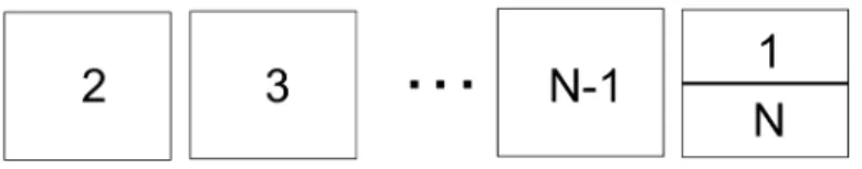
Assume we have a set J of N jobs such that p1 ≤ p2 ≤ · · · ≤pN. When all the
jobs fit in the space simultaneously, irrespective of the difference in their processing
times pj they are placed in the same batch. So Z =
P
j∈Jpj. If none of the jobs
each job is its own batch and Z =PN j=1
Pj
i=1pi. Smith 1956 proved that ordering
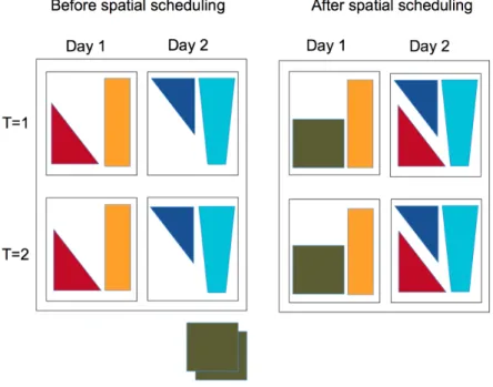
jobs in the nondecreasing sequence of their processing times is optimal for SMS. In general, while minimizing the sum of completion times, the more jobs we can fit earlier in our schedule the lower the objective. Therefore, it seems intuitive to always group jobs together rather than assign them to individual batches. Consider an instance of SSP with W=H=3 and job data as given in Table 2. We see that jobs 1 and 3 are the only jobs that fit the space simultaneously.
Table 2. Example instance with three jobs such that only jobs 1 and 3 simultaneously fit the space
Job Width Height 1 3 2 2 2 3 3 3 1
Let the processing times [p1, p2, p3] = [2, 3, 7] and let us assume we schedule
the batch with the lowest processing time first. We define batch processing time as the maximum processing time of jobs in a batch. Therefore, the batch sequence is
{2} and {1,3} as seen in Figure 2(a). Then the objective value for batched jobs is
calculated as Z = p1 + 3p2 +p3 =2 + 9 + 7 = 18. Alternately, if we schedule the
batches in their own batch, the sequence is {1},{2},{3} as seen in Figure 2(b) and
Z = 3p1+ 2p2+p3 = 6 + 6 + 7 = 19. This shows that grouping jobs can result in a
lower sum of completion times objective.
(a) Batching (b) No Batching
Now suppose, [p1, p2, p3] = [2, 5, 20]. When jobs 1 and 3 are batched, Z =
p1+ 3p2+p3 = 2 + 15 + 20 = 37. Without batching,Z = 3p1+ 2p2+p3 = 6 + 10 +
20 = 36. Thus in scenarios where jobs with large differences in processing times are grouped together, the batching approach does not necessarily lead to improvement in the objective.
Proposition 1 For N jobs, assume thatp1 < p2 <· · ·< pN−1 < pN. When jobs with both the largest and smallest processing times are assigned to the same batch, that is
{1, N}form a batch, and (N−1)p1−p2− · · · −pN−1 <0, the sum of completion times obtained by batching is greater than the objective value obtained without batching.
Fig. 3. Sequence in which batches are scheduled for Proposition1
Proof: Let P j∈J
Cjb be the sum of completion times obtained when batching and
P j∈J
Cn
j be the sum of completion times obtained without batching. Jobs {1, N} form
a batch, while the other jobs are each assigned individual batches. Since p1 < p2 <
· · ·< pN−1 < pN, batch{1, N} is processed at the end of the schedule (see Figure 3).
So P
j∈J Cb
j =p1+N p2+· · ·+ 3pN−1+pN. If each job is assigned its own batch, then P j∈J Cn j = N p1+ (N −1)p2+· · ·+ 2pN−1+pN. Therefore, P j∈J Cjb - P j∈J Cjn =[p1+N p2+· · ·+ 3pN−1+pN]−[N p1+ (N −1)p2+· · ·+ 2pN−1+pN] =(N −1)p1−p2− · · · −pN−1
(a) Batch Sequence (b) Alt. Sequence Fig. 4. Comparing strategies for sequencing batches
This contradicts the notion of scheduling as many jobs earlier in the schedule to minimize our objective. So, our intuitions about general scheduling problems do not always apply directly to problems with spatial resources. Batching seems to be beneficial only when processing times are similar.
Let us now look at the example with [p1, p2, p3] = [2, 3, 5]. If we schedule batches
in the sequence is{2}and{1,3}as seen in Figure 4(a), the objective Z=p1+ 3p2+p3
= 2 + 9 + 5 = 16. Instead, if we were to schedule the batches in the sequence{1,3}
then {2} as seen in Figure 4(b),Z= p1+p2+ 2p3 = 2 + 3 + 10 = 15. This suggests
that scheduling the jobs in the increasing order of batch processing times is not always effective.
Proposition 2 Consider a set J of N jobs such that p1 < p2 <· · ·< pN−1 < pN. If m of those jobs are in a batchB, including Job 1 and JobN, andpn> mpi,∀i∈J\B, then placing batch B at the end of a schedule provides a better objective than placing it at the beginning of the schedule.
Proof: Let P j∈J
Cb
j be the sum of completion times obtained when processing batchB
at the end of the schedule and P
j∈J
Cja be the sum of completion times obtained using
an alternate sequencing of batches (batch B is the first batch to be scheduled). Let
{1, u1, u2,· · · , um−2, N} be the m jobs in batchB such that p1 < p2 <· · ·< pu1−1 < pu1 < pu2 <· · ·< pum−2 < pum−1 <· · ·< pN.
{2},{3},· · · ,{u1−1},· · · ,{um−1},· · · ,{N−1},{B}.
So P
j∈J
Cjb = (p1+pu1+pu2+· · ·+pum−2+pN) + (N p2+ (N−1)p3+· · ·+ (m+ 1)pN−1).
Alternately, if we place batch B at the beginning of the schedule, P
j∈J Cja is given by (p1+pu1+pu2+· · ·+pum−2 + (N−m+1)pN + (N−m)p2+(N−m−1)p3+· · ·+pN−1). Therefore, P j∈J Ca j − P j∈J Cb j = [(p1+pu1 +pu2 +· · ·+pum−2 + (N−m+ 1)pN + (N −m)p2+ (N −m−1)p3+· · ·+pN−1)]− [(p1+pu1 +pu2 +· · ·+pum−2 +pN) + (N p2+ (N−1)p3+· · ·+ (m+ 1)pN−1)] =−mp2−mp3 − · · · −mpN−1+ (N −m)pN
Hence, when pN > mp2, pN > mp3,· · ·, pN > mpN−1, the result follows. 2
These results are useful in gaining an insight into the characteristics of spatial scheduling problems, thereby resulting in the development of more efficient algorithms and strategies to approximate its solutions.
3.1.1 Forming the Batches
When forming the batches, based on our previous analysis, we observe that plac-ing jobs with the smallest and largest processplac-ing times in the same batch does not necessarily result in a good batching scheme. So, we group jobs similar in processing time that also efficiently utilize the space to form a batch. We present two MIP mod-els, iterative and efficient area, that identify the assignment of jobs to batches. The objective for the iterative model is to minimize the maximum difference in processing times among jobs for each batch. The efficient area model extends this idea by also minimizing the total unused area in each batch. Both MlP formulations have been
adapted from the 2DBP model found in Pisinger and Sigurd 2005. Let J denote the
the number of batches equals the number of jobs (N).
3.1.1.1 Iterative model
In the iterative model (M1), we add a constraint to limit the number of batches
(S) being used by the model. The strategy is to iterate through possible values for
S, starting at S =N −1 and decreasing by 1 in each iteration. From the set of all
solutions, we can then chose the batching that results in the lowest sum of completion times objective value. The formulation for the iterative model is given by,
minX b∈B (Zmaxb−Zminb) (3.1) X b∈B rjb = 1 ∀j∈J (3.2) xj+wj ≤W ∀j∈J (3.3) yj+hj ≤H ∀j∈J (3.4) xi+wi−xj ≤W(1−lij) ∀i, j∈J, i < j, b∈B (3.5) yi+hi−yj ≤H(1−bij) ∀i, j∈J, i < j, b∈B (3.6) lij +lji+bij +bji+ (1−rib) + (1−rjb)≥1 ∀i, j∈J, b∈B (3.7) Zminb ≤(pj−M)rjb+M qb ∀j∈J, b∈B (3.8) Zmaxb ≥pjrjb ∀j∈J, b∈B (3.9) rjb≤qb ∀j∈J, b∈B (3.10) X j∈J rjb−qb ≥0 ∀b∈B (3.11) X b∈B qb =S (3.12) xj, yj ≥0 ∀j∈J (3.13) Zminb, Zmaxb ≥0 ∀b∈B (3.14) lij, bij ∈ {0,1} ∀i, j∈J (3.15) rjb ∈ {0,1} ∀j∈J, b∈B (3.16) qb ∈ {0,1} ∀b∈B (3.17) where,
B is the set of all batches
xj is the x-coordinate of job j ∈J
yj is the y-coordinate of job j ∈J
Zmaxb is the maximum processing time of jobs in batch b ∈B
Zminb is the minimum processing time of jobs in batchb ∈B
rjb = 1 if job j is in batch b 0 otherwise lij =
1 if job i is to the left of job j 0 otherwise bij =
1 if job i is below job j 0 otherwise qb = 1 if batch b is nonempty 0 otherwise For i, j ∈J and b ∈B.
Here, constraint (3.2) ensures that each job is assigned to only one batch. Constraints (3.3) and (3.4) ensure that jobs do not exceed the width and height of the space. We use constraints (3.5), (3.6), and (3.7) to prevent overlap of jobs within the space. Constraint (3.8) determines the minimum processing time within a batch, while (3.9)
identifies the maximum processing time for each batch. If job j is in batchb (rjb = 1)
then constraint (3.10) makes sure batch b is non-empty (qb = 1). When no jobs
are present in a batch, constraint (3.11) ensures that the batch is empty or qb = 0.
Constraint (3.12) sets the number of batches to be used by the model to some value
3.1.1.2 Efficient Area model
While solving N − 1 instances of M1 for different values of S finds the best
possible batch assignment, the second approach or efficient area model (M2) proposes to solve just one MIP to decide when and where to place jobs. The efficient area model includes an area utilization component to the existing objective. So, model 2 minimizes the maximum difference in processing times and the amount of workspace area that remains unused for each batch. The formulation for the efficient area model is given by, minX b∈B (Zmaxb−Zminb+U Ab) (3.18) X b∈B rjb = 1 ∀j∈J (3.19) xj+wj ≤W ∀j∈J (3.20) yj+hj ≤H ∀j∈J (3.21) xi+wi−xj ≤W(1−lij) ∀i, j∈J, i < j, b∈B (3.22) yi+hi−yj ≤H(1−bij) ∀i, j∈J, i < j, b∈B (3.23) lij +lji+bij +bji+ (1−rib) + (1−rjb)≥1 ∀i, j∈J, b∈B (3.24) Zminb ≤(pj−M)rjb+M qb ∀j∈J, b∈B (3.25) Zmaxb ≥pjrjb ∀j∈J, b∈B (3.26) rjb≤qb ∀j∈J, b∈B (3.27) X j∈J rjb−qb ≥0 ∀b∈B (3.28) W Hqb− X j∈J wjhjrjb=U Ab ∀b∈B (3.29) xj, yj ≥0 ∀j∈J (3.30) Zminb, Zmaxb, U Ab ≥0 ∀b∈B (3.31) lij, bij ∈ {0,1} ∀i, j∈J (3.32) rjb ∈ {0,1} ∀j∈J, b∈B (3.33) qb ∈ {0,1} ∀b∈B (3.34) where,
B is the set of all batches
xj is the x-coordinate of job j ∈J
yj is the y-coordinate of job j ∈J
Zmaxb is the maximum processing time of jobs in batch b ∈B
Zminb is the minimum processing time of jobs in batchb ∈B
U Ab is the unused area in batch b ∈B
rjb = 1 if job j is in batch b 0 otherwise lij =
1 if job i is to the left of job j 0 otherwise bij =
1 if job i is below job j 0 otherwise qb = 1 if batch b is nonempty 0 otherwise For i, j ∈J and b ∈B.
Here, constraint (3.19) ensures that each job is assigned to only one batch. Constraints (3.20) and (3.21) ensure that jobs do not exceed the width and height of the space. We use constraints (3.22), (3.23), and (3.24) to prevent overlap of jobs within the space. Constraint (3.25) determines the minimum processing time within a batch,
while (3.26) identifies the maximum processing time for each batch. If jobjis in batch
b (rjb = 1) then constraint (3.27) makes sure batch b is non-empty (qb = 1). When
no jobs are present in a batch, constraint (3.28) ensures that the batch is empty or
qb = 0. Constraint (3.29) calculates the unused area for each batch b. We set = 0.5
3.1.2 Scheduling the batches
Once the batches are identified using either M1 or M2, it is also important to
decide the sequence in which to schedule the batches. Smith 1956 proved that the
shortest processing time (SPT) rule, ordering jobs in the nondecreasing sequence of their job processing times, is optimal for the single machine scheduling problem. The idea is that by scheduling shorter jobs earlier in the schedule, more jobs can finish early resulting in a smaller sum. For SSP, the rule translates to scheduling the batches
in the nondecreasing sequence of their batch processing times. For example, if P1 is
the maximum processing time of all jobs in batch 1 andP2 is the maximum processing
time of all jobs in batch 2; then batch 1 is scheduled before batch 2 if and only if
P1 ≤ P2. However, as noted before, there are instances for which this rule does not
necessarily provide a better objective value. Therefore, we also consider scheduling jobs in the non-decreasing order of the average batch processing times, or the average processing time of all the jobs in a batch. We indicate the two scheduling rules as MAX and AVG respectively.
3.1.3 Post processing algorithm
By solving each instance of SSP using the iterative and efficient area models, we determine the assignments of jobs to batches that minimizes the maximum difference in processing times while efficiently utilizing the workspace. With this information, we then schedule the batches by applying either the MAX or AVG rules. Once a schedule
is created, we calculate the sum of completion times for the jobs asZH = Pj∈JC
H j ,
where CH
j is the completion time for job j. With this batching algorithm, each job
must wait until the previous batch has completed before it can start processing. In reality there may be jobs in the current batch that finish processing before the final
job in the batch. This means that jobs in later batches may be able to start earlier in the schedule. Since neither MIP model takes into account the temporal dimension, we use the algorithm schedule update to incorporate this observation and improve
ZH. For each batch the algorithm determines if jobs can start processing earlier in
the schedule. If jobj can be moved ahead in time by saytj units, then the completion
time is updated as, ˆCj = CjH −tj and ˆZ = P
j∈JCˆj is the new objective value.
Algorithm 1schedule update 1: Batch Sequence, b←1,2,· · · , m
2: Jb ←Set of jobs in batch b
3: Cj ←Completion time of job j
4: aheadj ←0,∀j∈J
5: for b= 2 to m do
6: forj∈Jb do
7: for t=Cj−pj−1 to 1do
8: if Space exists then
9: aheadj ←aheadj+ 1 10: f lag= 1 11: else 12: aheadj = 0 13: continue 14: end if 15: if aheadj >0then 16: if f lag = 1then 17: continue 18: else 19: break 20: end if 21: end if 22: end for 23: if f lag= 1 then 24: Cj ←Cj−aheadj 25: Update schedule 26: end if 27: end for 28: end for
3.2 Performance Analysis
In this section, we present solution guarantees on the objective valuesZH
gener-ated by the batch-scheduling algorithms. We refer toZOP T as the optimal objective
for the SSP formulation. We begin by analyzing instances with a set J of N jobs
such that at any given time k jobs can simultaneously fit the space (W ×H) and
p1 ≤p2 ≤ · · · ≤pN that define a special case of URCSP.
Theorem 1 When N=nk for anyn, k ∈Z∗
+, wj ≤W and hj =H ∀j ∈J, and p1 ≤ p2 ≤ · · · ≤ pN, if each batch has k jobs, then batch-scheduling is a k-approximation algorithm.
Proof: Let J denote the set of nk jobs and B the set of batches. Since p1 ≤ p2 ≤
· · · ≤ pN and we are minimizing the sum of completion times objective, we would
want to schedule jobs in the sequence 1,2,· · · , N. By design onlyk jobs can
simul-taneously fit the space. If the first k jobs are scheduled in a batch at the beginning
of the schedule, jobk+ 1 does not start until any of the jobs finish processing. The
first job to finish processing would be job 1. So completion time, Ck+1 = pk+1 +p1.
Applying this reasoning we note that a lower bound on the optimal objective for these instances is given by, ZOP T ≥Pnj=1(n−j+ 1)(pjk+pjk−1 +· · ·+pjk−k+1).
Since onlyk jobs can occupy the space at any given time, the number of batches
is nkk =n. If we use the MAX rule, Zb = maxj∈bpj ≥ pbk for each batch b ∈ B and
Z1 ≤ Z2 ≤ · · · ≤ Zn. Let us order the jobs in the sequence of the batches they are
assigned and in the increasing order of their processing times within each batch, so
that pbi now refers to the processing time of the ith job in batch b. It is important to
note here that pbi could be greater than thebi term in the sequencep1, p2, pbi,· · · , pN.
sum of its processing time and the completion times of the batches scheduled ahead ofj as:
CjH = pj, if job j≤k and
CjH =
pj+Zb−1+· · ·+Z1 if job j is in batch b and j>k
0 otherwise ZH = X j∈J CjH (3.35) = X j∈J pj+kZ1+k(Z1+Z2) +k(Z1+Z2+Z3) +· · ·+ +k(Z1+Z2+...+Zn−1) (3.36) = X j∈J pj+k[(n−1)Z1+ (n−2)Z2+· · ·+ 2Zn−2+Zn−1] (3.37) = X j∈J pj+k[(n−1)pk+ (n−2)p2k+· · ·+ +2p(n−2)k+p(n−1)k] (3.38) = n X j=1 (pjk−1+· · ·+pjk−k+1) + n X j=1 ((nk−jk+ 1)pjk) (3.39) = n X j=1 (pjk−1+· · ·+pjk−k+1) +k n X j=1 ((n−j+1 k)pjk) (3.40) = n X j=1 (pjk−1+· · ·+pjk−k+1) + n X j=1 ((n−j+ 1 k)pjk) +(k−1) n X j=1 ((n−j+ 1 k)pjk) (3.41) ≤ n X j=1 (pjk−1+· · ·+pjk−k+1) + n X j=1 ((n−j+ 1 k)pjk) +(k−1) n X j=1 ((n−j+ 1)pjk) (3.42) ≤ n X j=1 (pjk−1+· · ·+pjk−k+1) + n X j=1 ((n−j+ 1 k)pjk) +(k−1)ZOP T (3.43) ≤ ZOP T + (k−1)ZOP T (3.44) = kZOP T (3.45)
Equation (3.36) is obtained from the definition of completion times, CjH and we
get equation (3.38) per the definition of Zb. In each batch of k jobs, since the batch
processing time is pk, this is the only processing time included in the calculation
of completion times for the batches scheduled later. The processing times of the remaining (k-1) jobs are not repeated in this objective as seen in equation (3.39).
The bounds seen in (3.43) and (3.44) follow from the definition ofZOP T. 2
The bound shown helps us understand what makes instances of SSP hard. The real difficulty in solving instances of SSP lies in the spatial constraints as reflected
by the bound, which is dependent on k, the number of jobs you can simultaneously
fit within the given workspace. Notice that the bound is independent of the number of jobs. Also, recall that when minimizing the sum of completion times, we want to schedule more jobs earlier in the schedule. This is because the completion times of
a job includes the completion times of the jobs earlier in the schedule. When k = 1,
SSP reduces to SMS and our batching heuristic becomes SPT, which we know is
optimal (Smith 1956). Our bound depicts that ask increases, the solutions given by
the batch-scheduling algorithm may get larger than the optimal objective.
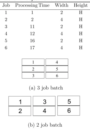
Consider the instance data with 6 jobs shown in Table 3 and a 10×10 workspace.
We can fit three jobs within the space, so the batches formed are {1,2,3} and
{4,5,6}as shown in Figure 5(a). The sum of completion times before post-processing,
ZH=p1+p2+4p3+p4+p5+p6 = 92. If we were to instead schedule the batches as seen
in Figure 5(b) in the sequence{1,2},{3,4}, and{5,6},ZH=p1+5p2+p3+3p4+p5+p6
= 91. Therefore, packing more jobs that are largely different in processing times be-cause they efficiently utilize the space does not result in a lower sum of completion times objective.
Table 3. SSP instance with N=6 jobs to depict that grouping more jobs in a batch does not guarantee lower objective value
Job Processing Time Width Height 1 1 2 H 2 2 4 H 3 11 2 H 4 12 4 H 5 16 2 H 6 17 4 H
(a) 3 job batch
(b) 2 job batch
Fig. 5. Example schedule with two and three jobs in a batch Proposition 3 For the instances defined by N=nk for any n, k ∈Z∗
+, wj = Wk and hj = H ∀j ∈ J, and p1 ≤ p2 ≤ · · · ≤ pN, after using the post-processing routine (schedule update), the sum of completion times objective Zˆ = ZOP T.
Proof: Considering the instances with N = nk jobs, let CjH, ˆCj, and CjOP T denote
the completion time for job j and ZH, ˆZ, and ZOP T denote the objective value for
the batch-scheduling algorithm, the post-processing routine, and the optimal solution
respectively. First, we observe that at any given time, k jobs can simultaneously fit
within the workspace, so there aren batches. So for all jobs j ≤k, ˆCj = CjOP T.
Let U ={u1, u2,· · · , uk}denote the k jobs in the next batch waiting to be scheduled,
time by saytj units, the new completion time is given by, ˆCj =CjH−tj. Since jobui
can be processed as soon asui−k completes and space becomes available, we get the
following recursive improvement on job completion times: ˆ Cui =C H ui −[(pui−1−pui−k) +· · ·+ (pk−p1)] ∀i∈ {1,· · · , k−1}and ˆ Cuk =C H uk So, ˆZ =ZH − Pn j=1 Pj i=1(pik−p(ik−k+1) = ZOP T 2 3.3 Computational Analysis
In this section we provide the computational results obtained by evaluating the two proposed procedures for solving the SSP and comparing it to the optimal solution. 3.3.1 Instance Generation
We tested both the iterative model (M1) and the efficient area model (M2) on
generated instances of SSP. The instance class denoted as N nP pRr < ABCD > i
hasn= 5 or 10 jobs, processing times generated in the uniform interval of (1, p) with
workspace area dimension W = H = r. The value for r is 10 or 20 units and i is
an instance indicator. A, B, C classifiers are used to indicate the distributions from which the width and height of jobs are sampled.
Class A wj ∈ Uniform Discrete [1,W2 ] andhj ∈ Uniform Discrete [1, H2]
Class B wj ∈ Uniform Discrete [1,W2 ] and hj ∈ Uniform Discrete [H2,H]
Class C wj ∈ Uniform Discrete [W2,W] and hj ∈ Uniform Discrete [H2,H]
Five instances of each class-type were generated, resulting in a total of 60 in-stances. All of the instances had jobs sorted in the increasing order of processing
times. Instances in Class C have jobs that occupy more than half the area. This results in each job getting its individual batch and SSP reduces to SMS which can be solved to optimality. So for the computational analysis we only consider instances in classes A and B. By design, instances in Class B should be relatively harder to solve than instances in class A. This is because all of the jobs in class A are small com-pared to the dimensions of the workspace, so we can fit more jobs together. Difficult instances of the problem occur, when some jobs are small and some are large (Class B).
Larger instances were obtained from Garcia 2010. The instances have 100, 500,
and 1000 jobs with a 10×7 workspace. For each job:
wj ∈U nif ormDiscrete[1,10]
hj ∈U nif ormDiscrete[1,7]
pj ∈U nif ormDiscrete[5,25]
Since we did not permit rotation of jobs, we had to interchange the widths and heights in certain cases to ensure that the jobs would fit within the space.
3.3.2 Valid Values for T
Recall that T represents the maximum completion time of a schedule, which is also seen in equation (4) of the SSP IP formulation found in Chapter 2. In order to guarantee that the model solves efficiently, it is important to make an appropriate choice for the value of T, especially for large instances.
For the instance classes A and B, the values for T were determined based on
bin packing. In Class A, the values for wj and hj in the worst-case are W2 and H2
Since jobs also have processing times, we need to stretch the bins to accommodate
the duration. Again, worst case the jobs in the bins are the last N4 jobs. Since
p1 < p2 <· · ·< pN, class A instances haveT ≤pd3N
4 e+· · ·+pN. A similar reasoning
is used for instance class B where T ≤pdN
2e
+· · ·+pN.
For larger instances, we make use of the previously discussed bound for bin
pack-ing to determine K, the maximum number of bins required to continuously pack the
jobs. Assuming, without loss of generality, that p1 < p2 < · · · < pN, we then have T ≤pn+1−2K+· · ·+pN, where K = min{ PN j=1hj H , PN j=1wj W
}. A valid value of T was determined as the
mini-mum of this bin packing based upper bound and sum of processing times. 3.3.3 Initial feasible solution heuristic
Table 4. Problem size comparisons between M1, M2, and original SSP MIP models
for N job instances
Model Number of Variables Number of Constraints M1 5N+ 2N2 N3+ 3N2+ 4N+ 1 M2 6N+ 3N2 N3+ 3N2+ 5N OPT 3N+ 3N2 4N2−2N
The motivation behind creating the batching models (M1 and M2) was to re-duce the size of the original SSP by looking only at the packing component of the problem. Nevertheless, we need to understand that M1 and M2 are still MIPs and as the instances grow larger, these models could take longer to solve to optimality. Table 4 shows a comparison of the number of variables and constraints between the SSP MIP formulation and the two batching models M1 and M2 for instances with
Algorithm 2simple pack 1: Batch←1 2: Job←1 3: while J ob≤N do 4: Begin: 5: x,y←0
6: if SpaceReqd[J ob]≤SpaceAvail[Batch]then
7: Loop X:
8: for i=x tox+wj do
9: Loop Y:
10: for j=y toy+hj do
11: if Height units are availablethen
12: x←x + 1
13: gotoLoop X
14: else
15: if Height units are unavailablethen
16: y←y + 1
17: gotoLoop Y
18: end if
19: end if
20: end for
21: if Width units are also available then
22: Assign space to job
23: Assign job to batch
24: else
25: if Width units are unavailable then
26: x←x + 1
27: gotoLoop X
28: end if
29: end if
30: end for
31: if Area is available but job cannot be fit in the given spacethen
32: Batch=Batch+ 1 33: gotoBegin 34: end if 35: else 36: Batch=Batch+ 1 37: gotoBegin 38: end if 39: Job←Job + 1 40: end while
guarantee an optimal solution to SSP. In order to improve the solution time for these MIP formulations, we provide the solver with an initial feasible solution obtained from a packing heuristic (simple pack). The pseudocode for simple pack is presented below. Basically, we start with an instance of SSP sorted in the increasing order of
job processing times, i.e. p1 ≤ p2 ≤ · · · ≤ pN. We sequentially begin grouping jobs
into a batch until they fit the space. Once the job can no longer fit the space, we create a new batch. This process is repeated until all jobs are assigned a batch.
3.3.4 Computational Results
In this section, we compare the solutions generated by the batch-scheduling ap-proaches (iterative and efficient area models) to the optimal solution (OPT) obtained by solving the mixed-integer program for SSP. The batching MIPs, M1 and M2, and the SSP MIP formulation were all implemented using the C programming language and solved using Gurobi 5.0 with a thread count of 1 and cuts parameter set to de-fault on a RedHat Enterprise 6.5 x86 64 server. The following tables compare the objective values and runtimes for the forty small instances with 5 jobs and 10 jobs and the large instances with 25 and 100 jobs (defined at the beginning of 3.3).
Table 5 lists the objective values obtained from solving instances with 5 and 10 jobs for M1 and M2 using the MAX rule and the optimal solution (OPT) for the original MIP formulation of SSP. Note that the objective reported for M1 is the best
possible value among theN−1 potential solutions it obtains and the run time is the
total time taken to iteratively solve all of the models. We observe that M2 seems to perform at least as well as M1, and both models return values close to the optimal solution. For these set of instances, the objective values returned by both models for
Table 5. Comparison of objectives obtained from M1, M2, and OPT for small instances of batch-scheduling
Instance M1 (Best) M2 OPT M1/OPTFactorsM2/OPT N5P10R10A 27 27 27 1.00 1.00 N5P19R10B 33 33 29 1.14 1.14 N5P10R20A 26 26 26 1.00 1.00 N5P10R20B 26 25 23 1.13 1.12 N10P10R10A 49 49 49 1.00 1.00 N10P10R10B 80 72 66 1.22 1.10 N10P10R20A 54 54 51 1.05 1.05 N10P10R20B 101 88 77 1.31 1.14
the MAX and AVG rules were identical for instances with five jobs and ten jobs.
Table 6. Comparison of M1, M2, and OPT runtimes for small instances of batch-scheduling Instance Runtime (seconds) M1 (Total) M2 OPT N5P10R10A 0.19 0.01 0.01 N5P19R10B 0.14 0.04 0.02 N5P10R20A 0.17 0.01 0.01 N5P10R20B 0.13 0.07 0.01 N10P10R10A 43.98 0.11 0.03 N10P10R10B 110.21 82.79 287.69 N10P10R20A 300.81 0.23 0.30 N10P10R20B 223.26 114.17 244.33
Table 6 presents the runtimes for solving the instances with 5 and 10 jobs using M1, M2, and the original MIP formulation. We observe that with smaller number of jobs, all three methods produce results quickly. The runtimes for M1 are larger
because it iteratively solvesN−1 models for each instance withN jobs. The solution
times that are in bold face for M2 indicate that certain instances of that class took over an hour to solve. In the few cases where that occurred, the incumbent solution at the end of twenty minutes was reported.
Table 7. Comparison of objectives obtained from M1, M2, andZIP for large instances of batch-scheduling Instance Objective Factor M1 (Best) M2 (Updated) ZIP M1/ZIP M2/ZIP N25P25E11 1697 1421 1215 1.40 1.17 N25P25E12 1518 1409 1022 1.49 1.38 N25P25E13 2204 2046 1540 1.43 1.33 N25P25E14 1555 1292 995 1.56 1.30 N25P25H11 1819 1762 1353 1.34 1.30 N25P25H12 1587 1332 965 1.64 1.38 N25P25H13 1929 1712 1169 1.65 1.46 N25P25H14 1625 1525 1066 1.52 1.43 N100P25E1 34372 24495 28205 1.22 0.87 N100P25H1 45571 24919 27672 1.65 0.90
Table 8. Comparison of M1, M2, andZIP runtimes for large instances of
batch-schedul-ing Instance Runtime (seconds) M1 (Total) M2 (Updated) ZIP N25P25E11 1920.00 1200.00 1200.00 N25P25E12 2280.00 1200.00 1200.00 N25P25E13 1920.00 1200.00 1200.00 N25P25E14 2040.00 1200.00 1200.00 N25P25H11 1800.00 1200.00 1200.00 N25P25H12 2160.00 1200.00 1200.00 N25P25H13 2040.00 1200.00 1200.00 N25P25H14 1800.00 1200.00 1200.00 N100P25E1 >3000.00 1200.00 1200.00 N100P25H1 >3000.00 1200.00 1200.00
Tables 7 and 8 list the objective values and runtimes obtained from solving larger instances (25 and 100 jobs) for M1 and M2 using the MAX rule and the objective
ZIP for the original MIP formulation of SSP. Note that the objective reported for
M1 is the best possible value among the N −1 potential solutions it obtains, with