Simulation for chaos game representation of genomes by recurrent iterated function systems

This is the author’s version of a work that was submitted/accepted for

pub-lication in the following source:

Yu, Zuguo

, Shi, Long, Xiao, QianJun, &

Anh, Vo V.

(2008) Simulation for

chaos game representation of genomes by recurrent iterated function

sys-tems.

Journal of Biomedical Science and Engineering,

1(1), pp. 44-51.

This file was downloaded from:

http://eprints.qut.edu.au/17206/

c

Copyright 2008 Scientific Research Publishing

Notice

:

Changes introduced as a result of publishing processes such as

copy-editing and formatting may not be reflected in this document. For a

definitive version of this work, please refer to the published source:

Simulation for chaos game representation of genomes

by recurrent iterated function systems

Zu-Guo Yu

1,2,*

, Long Shi

1

, Qian-Jun Xiao

1

and Vo Anh

2

1

School of Mathematics and Computational Science, Xiangtan University,

Hunan 411105, China.

2

School of Mathematical Sciences, Queensland University of Technology,

GPO Box 2434, Brisbane, Q 4001, Australia.

*

Corresponding author,E-mail: [email protected]

Abstract

Chaos game representation (CGR) of DNA sequences and linked protein sequences from genomes was proposed by Jeffrey (1990) and Yu et al. (2004), respectively. In this paper, we consider the CGR of three kinds of sequences from complete genomes: whole genome DNA sequences, linked coding DNA sequences and linked protein sequences. Some fractal patterns are found in these CGRs. A recurrent iterated function systems (RIFS) model is proposed to simulate the CGRs of these sequences from genomes and their induced measures. Numerical results on 50 genomes show that the RIFS model can simulate very well the CGRs and their induced measures. The parameters estimated in the RIFS model reflect information on species classification.

Keywords: Genomes; chaos game representation; recurrent iterated function systems.

1. Introduction

The hereditary information of organisms (except for RNA-viruses) is encoded in their DNA sequences which are one-dimensional unbranched polymers made up from four different kinds of monomers (nucleotides): adenine (a), cytosine (c), guanine (g), and thymine (t). Based on a technique from chaotic dynamics, Jeffrey (1990) proposed a chaos game representation (CGR) of DNA sequences by using the four vertices of a square in the plane to represent a,c,g and t. The method produces a plot of a DNA sequence which displays both local and global patterns. Self-similarity or fractal structures were found in these plots. Some open questions from the biological point of view based on the CGR were proposed (Jeffrey 1990).

If the DNA sequence were a random collection of bases, the CGR would be a uniformly filled square, conversely, any patterns visible in the CGR represent some pattern (information) in the DNA sequence (Goldman 1993). Goldman (1993) interpreted the CGRs in a biologically meaningful way. All points plotted within a quadrant must corresponding to subsequences of the DNA sequence that end with the base labelling the

corner of that quadrant. He also proposed a discrete time Markov Chain model to simulate the CGR of DNA sequences and use the sequence’s dinucleotide and trinucleotide frequencies to calculate the probabilities in these models. Goldman’s Markov model can be calculated directly and easily from the raw DNA sequences, without reference to the CGR.

Deschavanne et al. (1999) used CGR of genomes to discuss the classification of species. Almeida et al. (2001) showed the distribution of positions in the CGR plane is a generalization of Markov Chain probability tables that accommodates non-integer orders. Joseph and Sasikumar (2006) proposed a fast algorithm for identifying all local alignments between two genome sequences using the sequence information contained in their CGR.

Twenty different kinds of amino acids are found in proteins. The idea of CGR of DNA sequences proposed by Jeffrey (1990) was generalized and applied for visualizing and analyzing protein databases by Fiser et al. (1994). Generalization of CGR of DNA may take place in several ways. In the simplest case, the square in CGR of DNA is replaced by an n-sided regular polygon (n-gon), where n is the number of different elements in the sequence to be represented. As proteins consist of 20 kinds of amino acids, a 20-sided regular polygon (regular 20-gon) is the most adequate for protein sequence representation. A few thousand points result in an 'attractor' which gives a visualization of the rare or frequent residues and sequence motifs. Fiser et al. (1994) pointed out that the chaos game representation can also be used to study 3D structures of proteins.

Basu et al. (1998) proposed a new method for the chaos game representation of different families of proteins. Using concatenated amino acid sequences of proteins belonging to a particular family and a 12-sided regular polygon, each vertex of which represents a group of amino acid residues leading to conservative substitutions, the method generates the CGR of the family and allows pictorial representation of the pattern characterizing the family. Basu et al. (1998) found that the CGRs of different protein families exhibit distinct visually identifiable patterns. This implies that different functional classes of proteins produce specific statistical

biases in the distribution of different mono-, di-, tri-, or higher order peptides along their primary sequences. A well-known model of protein sequence analysis is the HP model proposed by Dill et al. (1985). In this model 20 kinds of amino acids are divided into two types, hydrophobic (H) (or non-polar) and polar (P) (or hydrophilic). But the HP model may be too simple and lacks sufficient information on the heterogeneity and the complexity of the natural set of residues (Wang and Wang 2000). According to Brown (1998), one can divide the polar class in the HP model into three classes: positive polar, uncharged polar and negative polar. So 20 different kinds of amino acids can be divided into four classes: non-polar, negative polar, uncharged polar and positive polar. In this model, one considers more details than in the HP model. We call this model a detailed HP model (Yu et al.2004a). Based on the detailed HP model, we proposed a CGR for the linked protein sequences from the genomes (Yu et al. 2004b).

The recurrent iterated function system in fractal theory (Barnsley and Demko, 1985; Falconer, 1997) has been applied successfully to fractal image construction (Barnsley and Demko, 1985; Vrscay, 1991), one dimensional measure representation of genomes (Anh et al. 2002; Yu et al. 2001, 2003) and magnetic field data (Wanliss et al. 2005; Anh et al. 2005) for example. Yu et al. (2007) proposed a CGR for the magnetic field data and used the RIFS model to simulate the CGR.

Although we proposed the CGR for linked protein sequences from genomes (Yu et al. 2004b), we did not consider how to simulate the CGRs. In this paper, we extend the CGR to the study of whole-genome DNA sequences and linked coding DNA sequences from genomes. Then we use the RIFS model to simulate the CGR of these 3 kinds of data from genomes and their induced measures. The probability matrix in our RIFS model is similar to the one in Markov model used by Goldman (1993), but the way to estimate this matrix is different.

2. Chaos game representation of genomes

Three kinds of sequences from complete genomes are considered, namely, whole-genome DNA sequences (including protein-coding and non-coding regions), linked sequences of all protein-coding DNA sequences and linked sequences of all protein sequences from complete genomes.

For DNA sequences, the CGR is obtained by using the four vertices of a square in the plane to represent a,c,g and t (Jeffrey 1990). The first point of the plot is placed half way between the center of the square and the vertex corresponding to the first letter, the ith point of the plot is placed half way between the (i-1)th point and the vertex corresponding to the ith letter in the DNA sequence.

For linked protein sequences, we outline here the way to get the CGR from Yu et al. (2004b). The protein

sequence is formed by twenty different kinds of amino acids, namely Alanine (A), Arginine (R), Asparagine (N), Aspartic acid (D), Cysteine (C), Glutamic acid (E), Glutamine (Q), Glycine (G), Histidine (H), Isoleucine (I), Leucine (L), Lysine (K), Methionine (M), Phenylalanine (F), Proline (P), Serine (S), Threonine (T), Tryptophan (W), Tyrosine (Y) and Valine (V) (Brown 1998, page 109). In the detailed HP model, they can be divided into four classes: non-polar, negative polar, uncharged polar and positive polar. The eight residues A, I, L, M, F, P, W, V designate the non-polar class; the two residues D, E designate the negative polar class; the seven residues N, C, Q, G, S, T, Y designate the uncharged polar class; and the remaining three residues R, H, K designate the positive polar class.

For a given protein sequence

s

=

s

1

...

s

_l with length l, where

s

_i is one of the twenty kinds of amino acids for

l

i

=

1

,...,

, we define        − − − − = , , 3 , arg , 2 , , 1 , , 0 polar positive is s if polar ed unch is s if polar negative is s if polar non is s if a i i i i i (1)

We then obtain a sequence

X

(

s

)

=

a

1

...

a

_l, where

a

i

is a letter of the alphabet {0,1,2,3}. We next define the CRG for a sequence X(s) in a square [0,1]

×

[ 0,1], where the four vertices correspond to the four letters 0,1,2,3: The first point of the plot is placed half way between the center of the square and the vertex corresponding to the first letter of the sequence X(s); the ith point of the plot is then placed half way between the (i-1)th point and the vertex corresponding to the ith letter. We then call the obtained plot the CGR of the protein sequence s based on the detailed HP model.

Figure 1. Chaos game representation of the linked protein sequence from genome of Mycobacterium tuberculosis CDC1551(MtubC) (with 1325681 amino acids)

0.2 0.4 0.6 0.8 1 0.2 0.4 0.6 0.8 1 0 0.5 1 1.5 2 2.5 3 3.5 4 x 10−3 x For MtubC−protein CGR y Measure µ

Figure 2. The measure

µ

based on a 128

×

128 mesh of the CGR in Figure 1.

Usually whole-genome DNA sequences and linked coding DNA sequences are relatively long, hence the resulting CGRs are too dense to visualize any pattern directly. The linked protein sequences are 3 times shorter than the linked coding DNA sequences, and their CGRs produce clearer self-similar patterns. For example, we show the CGR of the linked protein sequence of the bacterium Mycobacterium tuberculosis CDC1551 (MtubC) in Figure 1.

Considering the points in a CGR of an organism, we define a measure

µ

by

µ

(

B

)

=

#

(

B

)

/

N

_l , where

)

(

# B

is the number of points lying in a subset B of the CGR and

N

_lis the length of the sequence. We divide the square [0,1]

×

[0,1] into meshes of sizes 64

×

64, 128

×

128, 512

×

512 or 1024

×

1024. This results in a measure for each mesh. We then obtain a 64

×

64, 128

×

128, 512

×

512 or 1024

×

1024 matrix A

( )

kl J×J

=

µ

, where

J

=

64

,

128

,

512

or 1024, each element

µ

_klis the measure value on the corresponding mesh. We call A the measure matrix of the organism. The measure

µ

based on a 128

×

128 mesh on the CGRs are considered in this paper. For example, the measure

µ

based on a 128

×

128 mesh of the CGR in Figure 1 is shown in Figure 2.

3. Recurrent iterated function system for a

measure

Consider a system of contractive maps

}

,...,

,

{

S

1

S

2

S

N

S

=

and the associated matrix of probabilities P

=

(

p

_ij

)

such that

∑

=

1

j

p

ij ,

N

i

=

1

,

2

,...,

. We consider a random sequence generated by a dynamical system

x

n+1

=

S

σ_n

(

x

n

),

n

=

0

,

1

,

2

,...,

(2) where

x

₀ is any starting point and

σ

_nis chosen among the set

{

1

,

2

,...,

N

}

with a probability that depends on the previous index

σ

_n−1: _{n i}

i

p

i

P

_, 1

)

(

−

=

=

_σ

σ

. Then

(S, P) is called a recurrent iterated function system. Then there exist compact sets

A

,

A

_i,

i

=

1

,

2

,...,

N

such that

U

N i i

A

A

1 =

=

,

(

)

0 : j N p j i i

S

A

A

ji

U

>

=

where set

A

is called the attractor of the RIFS (S, P). A major result for RIFS is that there exists a unique invariant measure

µ

of the random walk (Eq. 2) whose support is

A

(Barnsley et al., 1989).

The coefficients in the contractive maps and the probabilities in the RIFS are the parameters to be estimated for the measure that we want to simulate. We now describe the method of moments to perform this task. In the two-dimensional case of our CGRs, we consider a system of N contractive maps

i

N

i

b

i

b

y

x

s

S

_{i i}

,

1

,

2

,...,

)

(

)

(

2 1

=













+













=

.

If

µ

is the invariant measure and

A

the attractor of the RIFS in R2, the moments of

µ

are

∫

∑∫

∑

= =

=

=

=

N i i mn i n N i A m n A m mn

x

y

d

x

y

d

g

g

i ₁ ) ( 1

µ

µ

.

Using the properties of the Markov operator defined by (S, P) (Vrscay, 1991), we get n _i A m i mn

x

y

d

g

i

µ

∫

=

) ( m _j n _j A j N j ji

s

x

b

j

s

y

b

j

d

p

j

µ

))

(

(

))

(

(

1 2 1

+

+

=

∑

∫

= j kl l n k m l k j m k n l N j ji

s

b

j

b

j

g

l

n

n

m

p

+ − − = = =

























=

∑

∑∑

₁

(

)

₂

(

)

0 0 1 . (3) When n=0, m=0, from

1

1 ) ( 00

=

∑

= N j j

g

we have ) ( 00 1 ) ( 00 j N j ji i

g

p

g

∑

=

=

⇒

(

)

₀₀( )

0

1

=

−

∑

= j ji N j ji

g

p

δ

(4) for

i

=

1

,

2

,...,

N

. Then we can get the values for

g

00(j)

,

j

=

1

,

2

,...,

N

by solving the above linear equations.

_{2 0}( ) 0 1 ) ( 0

(

)

j l l n l j n l N j ji i n

s

b

j

g

l

n

p

g

− = =

∑

∑













=

,

hence the moments are given by the solution of the linear equations ₀( ) 1

)

(

_{ji n}j N j ji n j

p

g

s

−

δ

∑

=

(

)

₀( )

,

1

,...

.

1 0 1 2

j

g

i

N

b

s

l

n

_j l n l N j l n l j

=













−

=

∑

−

∑

= = − (5) When n=0,

m

≥

1

₁ (₀) 0 1 ) ( 0

(

)

j k k m k j m k N j ji i m

s

b

j

g

k

m

p

g

− = =

∑

∑













=

,

hence the moments are given by the solution of the linear equations (₀) 1

)

(

_{ji m}j N j ji m j

p

g

s

−

δ

∑

=

(

)

(₀)

,

1

,...

.

1 0 1 1

j

g

i

N

b

s

k

m

_j k m k N j k m k j

=













−

=

∑

−

∑

= = − ₍₆₎ When

m

,

n

≥

1

g

_mn(i)

=

_{1 2} ( ) 1 0 0 1

)

(

)

(

klj l n k m l k j m k n l N j ji

s

b

j

b

j

g

l

n

n

m

p

+ − − − = = =

























∑∑

∑

,

)

(

( ) 1 ) ( 2 1 0 1 j mn N j n m j ji j ml l n l m j n l N j ji

s

b

j

g

p

s

g

l

n

p

∑

∑

∑

= + − + − = =

+













+

hence the moments are given by the solution of the linear equations

∑

−

=

= + ( ) 1

)

(

_{ji mn}j N j ji n m j

p

g

s

δ

_{1 2} ( ) 1 1 0 1 0

)

(

)

(

m k n l _klj l k j N j ji m k n l

g

j

b

j

b

s

p

l

n

n

m

_{+ − −} = − = − =

∑

∑∑

























₂ ( ) 1 1 0

)

(

n l _mlj l m j N j ji n l

g

j

b

s

p

l

n

_{+ −} − − =

∑

∑













−

) ( 1 1 1 0

)

(

m k _knj n k j N j ji m k

g

j

b

s

p

k

m

_{+ −} − − =

∑

∑













−

, (7) for

i

=

1

,

2

,...,

N

. If we denote by

G

_mn the moments obtained directly from a given measure, and

g

_mnthe formal expression of moments obtained from the above formulae, then solving the optimization problem

2 , ), ( ), ( , ₁

min

₂

(

mn

)

n m mn p i b i b s_{i ij}

∑

g

−

G

will provide the estimates of the parameters of the RIFS.

Once the RIFS (

S

_i

(

x

),

p

_ij

,

i

,

j

=

1

,

2

,...,

N

) has been estimated, its invariant measure can be simulated in the following way: Generate the attractor of the RIFS via the random walk (Eq. 2). Let

χ

_B be the indicator function of a subset B of the attractor

A

. From the ergodic theorem for RIFS (Barnsley et al., 1989), the invariant measure is then given by













+

=

∑

= ∞ → n k k B n

n

x

B

0

)

(

1

1

lim

)

(

χ

µ

.

By definition, an RIFS describes the scale invariance of a measure. Hence a comparison of the given measure with the invariant measure simulated from the RIFS will confirm whether the given measure has this scaling behaviour. This comparison can be undertaken by computing the cumulative walk of a measure visualized as intensity values on a J

×

J mesh; here J=128 in this paper.

If we convert the two-dimensional matrix A

( )

kl J×J

=

µ

to an one dimensional vector by concatenate every row in A at the end of previous row. We denote the one-dimensional vector as

f

=

(

f

₁

,

f

₂

,...,

f

_J×J

)

. The cumulative walk is defined as

(

),

1

f

f

F

j i i j

=

∑

−

=

J

J

j

=

1

,

2

,...,

×

,

where

f

is the average value of all element in vector

f

. Returning to the CGR, an RIFS with 4 contractive maps

{

S

1

,

S

2

,

S

3

,

S

4

}

is fitted to the measure obtained from the CGR using the method of moments. Here we can fix













=

y

x

S

2

1

1 ,













+













=

5

.

0

0

2

1

2

y

x

S

,













+













=

5

.

0

5

.

0

2

1

3

y

x

S

,













+













=

0

5

.

0

2

1

4

y

x

S

.

Hence the parameters needed to be estimated are the probabilities in the matrix P. Once we have estimated the probability matrix in the RIFS, we can start from the point (0.5, 0.5) and use the chaos game algorithm Eq. (2) to generate a random point sequence

{

x

i

}

with the same length

N

_l of the whole- genome DNA sequence, linked coding DNA sequence or the linked protein sequence. Then the plot of the random point sequences is the RIFS simulation of the original CGR of the data. For example the RIFS simulated CGR of the CGR in Figure 1 is shown in Figure 3. Comparing the RIFS simulation in Figure 3 with the original CGR in Figure 1, it is apparent that they are quite similar. We then obtain the 128

×

128 mesh measure

µ

'

based on the simulated CGR. The

Figure 3. The RIFS simulated CGR for the CGR in Figure 1. 0.2 0.4 0.6 0.8 1 0.2 0.4 0.6 0.8 1 0 0.5 1 1.5 2 2.5 3 3.5 4 x 10−3 x

For MtubC−protein RIFS CGR

y

Measure

µ

’

Figure 4. The measure

µ

'

based on a 128

×

128 mesh of the RIFS simulated CGR in Figure 3. measure

µ

'

can be regarded as a simulation of the measure

µ

induced from the original CGR. For example, we show the 128

×

128 mesh measure

µ

'

based on the simulated CGR of Figure 3 in Figure 4. The cumulative walks of these two measures can then be obtained to show the performance of the simulation.

We determine the goodness of fit of the measure simulated from the RIFS model relative to the original measure based on the following relative standard error (RSE) (Anh et al. 2002):

2 1

e

e

e

=

, where

∑

=

−

=

M j j j

F

F

M

e

1 2 1

(

)

1

)

, and

∑

=

−

=

M j ave j

F

F

M

e

1 2 2

(

)

1

.

Here

M

=

128

×

128

,

(

F

_j

)

M_j=1 and

(

F

)

_j

)

M_j=1are the walks of the original measure and the RIFS simulated measure respectively,

F

_aveis the mean value of

(

F

_j

)

M_j=1.

0 2000 4000 6000 8000 10000 12000 14000 16000 18000 0 0.005 0.01 0.015 0.02 0.025 0.03 0.035 0.04 0.045 0.05 Pixel position Walk representation Mtub−protein, e=0.0300

Walk for the original 128X128 measure Walk for the RIFS simulation

Figure 5. The walk representation of measures induced by the CGR in Figure 1 and its RIFS simulation in Figure 4.

The goodness

e

<

1

.

0

indicates the simulation is very well (Anh et al. 2002). For example, the cumulative walks for the measure induced by the CGR in Figure 1 and its RIFS simulation in Figure 4 are given in Figure 5. It is seen that the two walks are almost identical. This indicates that RIFS fits very well the measure induced by the original CGR. The RSE e=0.0300 is very small, which also indicates excellent fitting.

4. Data, discussion and conclusions

We downloaded whole-genome DNA sequences, coding DNA sequences and protein sequences from 50 complete genomes of Archaea and Eubacteria from the public database Genbank at the web site http://www.ncbi.nlm.nih.gov/Genbank/. We list the name of the 50 bacteria in Appendix.

We then produce the CGRs of the data from the 50 genomes as described in Section 2. For more examples, we plot the chaos game representation of the linked coding sequence from genome of Mycoplasma pulmonis UAB CTIP (Mpul) in Figure 6. Fractal (self-similarity) patterns can be seen in these CGRs. We only use the moments of 128

×

128 mesh measure

µ

based on the CGRs to estimate the parameters (probability matrix) in

the RIFS model. Then the RIFS simulation of the original CGRs is performed using the chaos game algorithm. We then get the 128

×

128 mesh measure

'

µ

based on the simulated CGR. To show the performance of the simulation, we compare the cumulative walks of the original measure and its simulation

µ

'

. For example, the RIFS simulated CGR of the linked coding sequence from genome of Mycoplasma pulmonis UAB CTIP (Mpul) based on the 128

×

128 mesh measure

µ

from Figure 6 is shown in Figure 7, while the the walk representation of measures induced by the CGR in Figure 6 and its RIFS simulation in Figure 7 are shown in Figure 8.

Figure 6. Chaos game representation of the linked coding sequence from genome of Mycoplasma pulmonis UAB CTIP (Mpul) (with 873,651 bps)

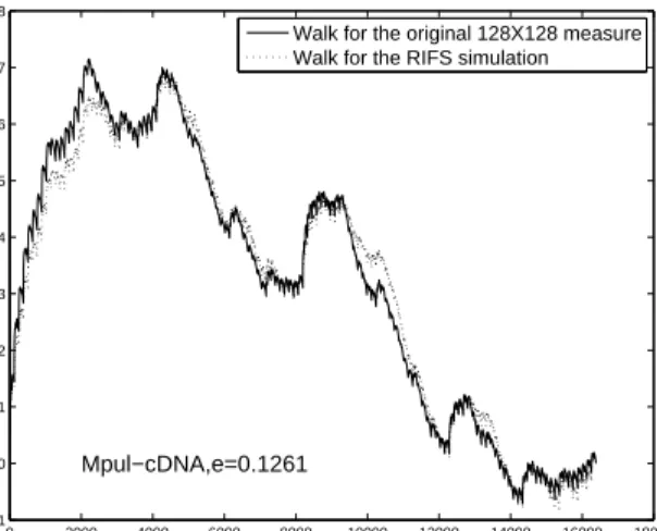
Figure 7. The RIFS simulated CGR for the CGR in Figure 6. 0 2000 4000 6000 8000 10000 12000 14000 16000 18000 −0.01 0 0.01 0.02 0.03 0.04 0.05 0.06 0.07 0.08 Pixel position Walk representation Mpul−cDNA,e=0.1261

Walk for the original 128X128 measure Walk for the RIFS simulation

Figure 8. The walk representation of measures induced by the CGR in Figure 6 and its RIFS simulation in Figure 7.

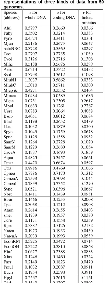
Goldman (1993) interpreted the patterns in CGRs of DNA sequences by the dinucleotide and trinucleotide frequencies in the original sequence. The probability matrix in our RIFS model characterizes the dinucleotide or di-amino acid frequencies (information) which is similar to the one in Markov model used by Goldman (1993), but the way to estimate this matrix is different. The values of the RSE of the simulation for 50 genomes are listed in Table 1.

It is seen that all the values of the RES except two are much less than 1.0, confirming that the RIFS model can simulate very well the measures of three kinds of data. The values of e for whole-genome DNA data are generally larger than those for linked coding DNA data, which in turn are larger than those for linked protein data. In other words, the RIFS model can simulate the measures for linked protein data better than the measures for linked coding DNA data, and can simulate measures for linked coding DNA data better than the measures for whole-genome DNA data. We notice that the linked protein sequence is shorter than the corresponding linked coding DNA sequence, while the linked coding DNA is shorter than the whole-genome sequence. We guess the length of the data reflects the information complexity of the data and the RIFS model is still simple model which simulates simpler data better. This result indicates that we can use the estimated parameters in the RIFS model for linked protein data from genomes to characterize the genomes. We find that the estimated probability matrices in the RIFS model for species from the same category are similar to each other. For example, the estimated probability matrices for the measures of linked protein sequences from the three Gram-positive Eubacteria (high G+C) Mycobacterium tuberculosis H37Rv (MtubH), Mycobacterium tuberculosis CDC1551 (MtubC) and Mycobacterium leprae TN (Mlep) are:

Table 1 The goodness of fit for the walk representations of three kinds of data from 50 genomes. Species (abbrev.) e for whole DNA e for coding DNA e for linked proteins Aful Paby Pyro Mjan haloNRC Taci Tvol Mthe 0.5797 0.3502 0.4324 0.2136 0.3728 0.2707 0.3126 0.5188 0.2669 0.3214 0.3411 0.2675 0.3569 0.2735 0.2716 0.5676 0.0366 0.0333 0.0361 0.0647 0.0297 0.1030 0.1308 0.0299 Aero Ssol 0.6213 0.3798 0.2222 0.3612 0.0452 0.1098 MtubH MtubC Mlep & 1.3037 1.3010 0.4271 0.5862 0.5711 0.3332 0.0333 0.0300 0.0404 Mpneu Mgen Mpul Uure Bsub Bhal Llac Spyo Spne SaurN SaurM CaceA 0.0484 0.0731 0.0639 0.0783 0.4051 0.1198 0.1032 0.1049 0.1125 0.1264 0.1229 0.1887 0.0589 0.2305 0.1261 0.2064 0.8012 0.2652 0.1879 0.1759 0.1358 0.2728 0.2680 0.1693 0.1686 0.2617 0.2267 0.4058 0.0684 0.0489 0.0500 0.0678 0.0932 0.1020 0.1054 0.1859 Aqua Tmar 0.4825 0.4470 0.3457 0.6674 0.0661 0.0597 Ctra Cpneu CpneuA CpneuJ 0.8986 0.7786 0.7593 0.7899 0.4769 0.7170 0.7093 0.7352 0.1066 0.1312 0.1044 0.1290 Syne Nost 0.0521 0.1411 0.0396 0.1439 0.0667 0.0931 Bbur Tpal 0.1466 0.3068 0.1255 0.1212 0.2008 0.0908 Atum smel Ccre Rpro 0.2614 0.1739 0.1171 0.3887 0.2655 0.1957 0.1558 0.7126 0.0403 0.0380 0.0259 0.2132 Nmen NmenA 0.1973 0.2039 0.1933 0.1993 0.0430 0.0559 EcoliKM EcoliOH Hinf Xfas Paer Pmul Buch 0.3225 0.3222 0.0677 0.1246 0.2149 0.1032 0.1954 0.3472 0.3810 0.2388 0.1460 0.1823 0.2087 0.2598 0.0714 0.0868 0.0883 0.0324 0.0470 0.0911 0.3911 Hpyl Cjej 0.2567 0.1540 0.2615 0.1797 0.1161 0.0802

























=

084086

.

0

127584

.

0

275576

.

0

139217

.

0

266087

.

0

354118

.

0

286638

.

0

215737

.

0

263546

.

0

096754

.

0

027692

.

0

149496

.

0

386300

.

0

421544

.

0

410094

.

0

495551

.

0

MtubH

P

























=

085164

.

0

135310

.

0

275647

.

0

138764

.

0

267148

.

0

344503

.

0

282788

.

0

218983

.

0

259119

.

0

101162

.

0

028024

.

0

146193

.

0

388569

.

0

419026

.

0

413542

.

0

496060

.

0

MtubC

P

























=

046717

.

0

156541

.

0

275709

.

0

140182

.

0

293543

.

0

313224

.

0

272109

.

0

226108

.

0

260004

.

0

123836

.

0

038055

.

0

143671

.

0

399737

.

0

406399

.

0

414127

.

0

490039

.

0

Mlep

P

Hence we can use the RIFS estimated probability matrices of the linked protein sequences from genomes to define a distance metric between two species for the purpose of construction of phylogenetic tree. This work is being undertaken.

We can now draw some conclusions. First, the chaos game representation of the three kinds of data from genomes can give a visualization of the genomes and produce some fractal patterns. Second, the RIFS model can be used to simulate CGRs of genomes and their induced measures. Third, the RIFS simulation of measures for linked protein data is better than that of measures for whole-genome DNA data and linked coding DNA data. Finally, the estimated parameters in the RIFS models for the linked protein data from genomes can be used to characterize the phylogenetic relationships of the genomes.

Acknowledgment

Financial support was provided by the Chinese National Natural Science Foundation (grant no. 30570426), Fok Ying Tung Education Foundation (grant no. 101004) and the Youth foundation of Educational Department of Hunan province in China (grant no. 05B007) (Z.-G. Yu), and the Australian Research Council (grant no. DP0559807) (V.V. Anh).

References

[1] J.S. Almeida, J.A. Carrico, A. Maretzek, P.A. Noble, M. Fletcher, “Analysis of genomic sequences by Chaos Game Representation”. Bioinformatics,17( 2001), pp 429-437. [2] V.V. Anh, K.S. Lau, and Z.G. Yu, “Recognition of an organism from fragments of its complete genome”, Phys. Rev.

[3] V.V. Anh, Z.G. Yu, J.A. Wanliss, and S.M. Watson, “Prediction of magnetic storm events using the Dst index”,

Nonlin. Processes Geophys., 12 (2005), pp. 799-806.

[4] M.F. Barnley, J.H. Elton, and D.P. Hardin, “Recurrent iterated function systems”, Constr. Approx. B, 5 (1989), pp. 3-31.

[5] M.F. Barnsley, and S. Demko, “Iterated function systems and the global construction of fractals”, Proc. R. Soc. London,

Ser. A, 399 (1985), pp. 243-275.

[6] S. Basu, A. Pan, C. Dutta and J. Das, “Chaos game representation of proteins”. J. Mol. Graphics and Modelling, 15 (1998), pp. 279-289.

[7] T.A. Brown, Genetics (3rd Edition). CHAPMAN & HALL, London, 1998.

[8] P.J. Deschavanne, A Giron, J. Vilain, G. Fagot and B. Fertil, “Genomics signature: Characterization and classification of species assessed by chaos game representation of sequences”. Mol. Biol. Evol. 16(1999),

pp 1391-1399.

[9] K.A.Dill, “Theory for the folding and stability of globular Proteins”, Biochemistry, 24 (1985), pp. 1501-1509.

[10] K. Falconer, Techniques in Fractal Geometry, Wiley, 1997.

[11] A. Fiser, GE Tusnady and I. Simon, “Chaos game representation of protein structures”. J. Mol. Graphics, 12 (1994), pp. 302-304.

[12] N. Goldman, “Nucleotide, dinucleotide and trinucleotide frequencies explain patterns observed in chaos game

representations of DNA sequences.” , Nucleic Acids Research, 1993, 21(10): (1993), pp. 2487-2491

[13] H.J. Jeffrey, “Chaos game representation of gene structure”. Nucleic Acids Research, 18(8): (1990), pp. 2163-2170.

[14] J.Joseph, R. Sasikumar, “Chaos game representation for comparision of whole genomes”. BMC Bioinformatics, 7(2006), pp 243: 1-10.

[15] E.R. Vrscay, “Iterated function systems: theory, applications and inverse problem”, in: Fractal Geometry and

Analysis, edited by: Belair, J. and Dubuc, S., Kluwer,

Dordrecht, pp. 405-468, 1991.

[16] J. Wang and W. Wang, “Modeling study on the validity of a possibly simplified representation of proteins”, Phys. Rev. E, 61 (2000), pp. 6981-6986.

[17] J.A. Wanliss, V.V. Anh, Z.G. Yu, and S. Watson, “Multifractal modelling of magnetic storms via symbolic dynamics analysis”, J. Geophys. Res., 110 (2005), art. no. A08214, pp. 1-11,.

[18] Z.G. Yu, V.V. Anh, and K.S. Lau, “Measure representation and multifractal analysis of complete genomes”, Phys. Rev. E, 64 (2001), art. no. 031903, pp. 1-9,.

[19] Z.G. Yu, V.V. Anh, and K.S. Lau, “Iterated function system and multifractal analysis of biological sequences”,

International J. Modern Physics B, 17: (2003), pp. 4367-4375.

[20] Z.G. Yu, V.V. Anh, and K.S. Lau, “Fractal analysis of large proteins based on the Detailed HP model”, Physica A, 337 (2004a), pp. 171-184.

[21] Z.G. Yu, V.V. Anh, and K.S. Lau, “Chaos game representation, and multifractal and correlation analysis of protein sequences from complete genome based on detailed HP model”, J. Theor. Biol., 226(3) (2004b), pp..341-348.

[22] Z.G. Yu, V.V. Anh, , J.A. Wanliss and S.M. Watson, “Chaos game representation of the Dst index and prediction of geomagnetic storm events”, Chaos, Solitons & Fractals, 31 (2007), pp. 736-746,

Appendix

These 50 bacteria include eight Archae Euryarchaeota: Archaeoglobus fulgidus DSM 4304 (Aful, NC000917), Pyrococcus abyssi GE5 (Paby, NC000868), Pyrococcus horikoshii OT3 (Pyro, NC000961), Methanococcus jannaschii DSM 2661 (Mjan, NC000909), Halobacterium sp. NRC-1 (haloNRC, NC002607), Thermoplasma acidophilum DSM 1728 (Taci, NC002578), Thermoplasma volcanium GSS1 (Tvol,NC002689), and Methanobacterium thermoautotrophicum deltaH (Mthe, NC000916); two Archae Crenarchaeota: Aeropyrum pernix K1 (Aero, NC000854) and Sulfolobus solfataricus P2 (Ssol, NC002754); three Gram-positive Eubacteria (high G+C): Mycobacterium tuberculosis H37Rv (MtubH, NC000962), Mycobacterium tuberculosis CDC1551 (MtubC, NC002755) and Mycobacterium leprae TN (Mlep, NC002677); twelve Gram-positive Eubacteria (low G+C): Mycoplasma pneumoniae M129 (Mpneu, NC000912), Mycoplasma genitalium G37 (Mgen, NC000908), Mycoplasma pulmonis UAB CTIP (Mpul, NC002771), Ureaplasma urealyticum serovar 3 str. ATCC 700970 (Uure, NC002162), Bacillus subtilis subsp. subtilis str. 168 (Bsub, NC000964), Bacillus halodurans C-125 (Bhal, NC002570), Lactococcus lactis subsp. lactis Il1403 (Llac, NC002662), Streptococcus pyogenes M1 GAS (Spyo, NC002737), Streptococcus pneumoniae TIGR4 (Spne, NC003028), Staphylococcus aureus subsp. aureus N315 (SaurN, NC002745), Staphylococcus aureus subsp. aureus Mu50 (SaurM, NC002758), and Clostridium acetobutylicum ATCC 824 (CaceA, NC003030). The others are Gram-negative Eubacteria, which consist of two hyperthermophilic bacteria: Aquifex aeolicus VF5 (Aqua, NC000918) and Thermotoga maritima MSB8 (Tmar, NC000853); four Chlamydia: Chlamydia

trachomatis D/UW-3/CX (Ctra, NC000117), Chlamydia pneumoniae CWL029 (Cpneu, NC000922), Chlamydia pneumoniae AR39 (CpneuA, NC002179) and Chlamydia pneumoniae J138 (CpneuJ, NC002491); two Cyanobacterium: Synechocystis sp. PCC6803 (Syne, NC000911) and Nostoc sp. PCC 7120 (Nost, NC003272); two Spirochaete: Borrelia burgdorferi B31 (Bbur, NC001318) and Treponema pallidum Nichols (Tpal, NC000919); and fifteen Proteobacteria. The fifteen Proteobacteria are divided into four subdivisions, namely alpha subdivision: Agrobacterium tumefaciens strain C58 (Atum, NC003062), Sinorhizobium meliloti 1021 (smel, NC003047), Caulobacter crescentus CB15 (Ccre, NC002696) and Rickettsia prowazekii Madrid (Rpro, NC000963); beta subdivision: Neisseria meningitidis MC58 (Nmen, NC003112) and Neisseria meningitidis Z2491 (NmenA, NC003116); gamma subdivision: Escherichia coli K-12 MG1655 (EcoliKM, NC000913), Escherichia coli O157:H7 EDL933 (EcoliOH, NC002695), Haemophilus influenzae Rd (Hinf, NC000907), Xylella fastidiosa 9a5c (Xfas, NC002488), Pseudomonas aeruginosa PA01 (Paer, NC002516), Pasteurella multocida subsp. multocida str. Pm70 (Pmul, NC002663) and Buchnera str. APS (Buch, NC002528); and epsilon subdivision: Helicobacter pylori 26695 (Hpyl, NC000915) and Campylobacter jejuni subsp. jejuni NCTC 11168 (Cjej, NC002163). The abbreviations in the brackets stand for the names of these species and their NCBI accession numbers.