Hold-up and sequential specific investments
Vladimir Smirnov and Andrew Wait
∗August 2001
Abstract
We explore the hold-up problem when trading parties can make specific investments simultaneously or sequentially. As previously emphasized in the literature, sequencing of investments can allow some projects to proceed that would not be feasible with a simultaneous regime. This is not always the case, however. A cost of sequencing investment is that it can disadvantage some parties, reducing their incentive to invest. The mere possibility of sequential investment can be detrimental to welfare; it can even prevent trade from occur-ring. This is a new result: it allows the choice about the timing of investment to be interpreted as a new form of hold-up. We also examine an investment game in which both parties would prefer to invest second (follow) rather than lead. This game displays some interesting dynamics. As the the number of potential investment periods is increased, the subgame perfect equilibrium can switch between a prisoners’ dilemma and a coordination game.
∗Economics Program, Research School of Social Sciences, Australian National University ACT
0200 AUSTRALIA and Department of Economics, University of Melbourne VIC 3010 AUSTRALIA. Email: vladimir.smirnov@anu.edu.au, await@coombs.anu.edu.au. The authors would like to thank Suren Basov, Steve Dowrick, Simon Grant, Martin Osborne, Rohan Pitchford, Matthew Ryan, Rhema Vaithianathan and participants at the Economic Theory Workshop, Australian National University and the Monday Workshop at the University of Melbourne. Any remaining errors are the authors.
1
Introduction
Many projects prior to their commencement are nebulous and difficult to describe.
For example, research and development projects often have vague objectives and
spec-ulative or uncertain outcomes; start-up firms are often based around intangible ideas.
With joint projects this makes it difficult to write a complete contract specifying the
tasks of each party and the desired outcome (see for example Hart 1995, pp. 1-5).
Grout (1984) and Hart (1995), amongst others, showed that parties may not make
efficient specific investments when contracts are incomplete.1 These models typically
have the following structure: trading parties make their investments that are sunk
and, at least partially, specific; after these investments are made contracting on some
relevant variable becomes possible; at this point the parties renegotiate and trade
oc-curs according to the renegotiated contract. If, because of renegotiation, a party does
not receive the full marginal return from their effort, investment will be inefficient.2
Other authors have examined how sequencing or staggering investment can help
alleviate the hold-up problem. For example, Neher (1999) considered staged financing
of a project when an entrepreneur is unable to commit not to renege on their contract
with the financier. When the project is financed in stages, as the project matures, the
alienable (contractible) element of the project, manifested in the accumulated physical
assets, provides a better bargaining position during renegotiation for the financier in
the event of default. As a consequence, the entrepreneur has less incentive to renege.
1Also see Grossman and Hart (1986) and Hart and Moore (1988).
2It has also been noted that the level of general investments can be effected in the presence of
incomplete contracts: Malcomson (1997) noted that hold-up of general investment can occur when there are turnover costs.
De Fraja (1999) considered the Stackelberg-type sequencing of investments in the
presence of hold-up. De Fraja’s solution to the hold-up problem required the first
party to make a general investment then make a take-it-or-leave-it offer to the other
party that included him paying for the specific investment.3 Given that this contract
makes the first party the residual claimant she will invest efficiently. Admati and
Perry (1991) showed two parties can overcome the free-rider problem by financing a
public good in stages.
The model presented here develops a simple framework to contrast the
simulta-neous and staged (sequential) investment regimes. The essence of the model is that
staging the project allows some investment to be made after the point in time when
a contract can be written. Here, the resolution of the incompleteness is facilitated by
the completion of some aspect of the project. For example, in Grossman and Hart
(1986) contracting became possible after the two parties made their initial investment.
Similarly, Neher (1999) made the point that contracting becomes progressively more
feasible as human capital invested in the project is converted into physical assets.
The basic structure of the model is as follows. Two parties are required to invest
in order to complete a project. Two distinct alternatives are possible. First, they
can invest simultaneously at the start of the game. If they do so, both invest prior
to complete contracting being possible. After both investments are sunk the parties
renegotiate and the payoffs are realised.4 Alternatively, one party can invest first
3Although the investment may be industry-specific, it is not relationship-specific in the traditional
sense. See Malcomson (1997).
4This regime is equivalent to the incomplete contract models of Grossman and Hart (1986), Hart
while the other party waits. This first investment allows the project to take shape:
as a result, contracting on the second investment becomes possible. At this stage, the
parties will renegotiate and write a contract specifying the second party’s investment.
The final stage of investment will then occur, completing the project and allowing
the parties to receive their payoffs.
Several important results arise from this simultaneous versus sequential investment
model. First, the sequential regime can create trading possibilities that may not be
feasible if the parties have to invest simultaneously. For example, the second player
will not be willing to invest simultaneously if it leaves them with a negative net return.
On the other hand, the sequential investment regime gives this player the opportunity
to delay their investment until when contracts are complete. This may be sufficient
incentive to encourage the seller to invest. This result is similar to the results of other
authors, for example Neher (1999) and Admati and Perry (1991), albeit in a different
context.
Second, we show that the possibility of investing sequentially does not always
improve welfare. As it turns out, flexibility in the timing of investment can act as
an additional form of hold-up. For want of a better expression we call this kind of
hold-up ‘follow-up’. This occurs when both parties should invest simultaneously at
the start of the project in order to maximise surplus but there is an incentive for one
party to wait until after the other player has sunk their effort before they follow-up
with their own investment.5 Consider the case when technology requires that one
particular party must invest at the commencement of a project but that the other
party can invest either at the same time or wait. The first party will anticipate that
the second party will delay their investment - opt for the sequential regime - if it suits
them.
Third, as discussed above, the second player acting in self-interest may have the
incentive to opt for the regime that does not maximise total welfare. The burden of
this opportunism is typically borne by the other player. However, if such opportunism
drives the first player’s return below his no-trade payoff, this additional form of
hold-up will prevent a potential surplus-enhancing project from proceeding. In this case,
the second player also bears some of the cost from the reduction in total surplus
-the second player is disadvantaged by her inability to commit to a particular timing
schedule of investment.
Fourth, the decision over the timing of investment can be seen as a choice over
the completeness of contracts: if parties opt for simultaneous investment they are
opting for a more incomplete contract than possible (with the sequential regime).
As a result, the choice concerning the completeness of contract is endogenous. The
advantage of a (more) complete contract with sequential investment is that hold-up
of the follower is avoided. The cost of a complete contract is that it diminishes the
first party’s incentive to invest and increase the costs of delay. The second party will
opt for simultaneous investment that is, they will opt for an incomplete contract
power they receive from avoiding hold-up.6
Finally, interesting dynamics can arise out of this investment game when both
parties want to be a follower rather than the leader. If there are just two potential
investment periods (and the opportunity to invest disappears after the second
pe-riod) the parties find themselves in a prisoners’ dilemma. If the potential investment
horizon is continually extended to three periods, four periods and so on, eventually
the benefit from not investing (waiting) will diminish sufficiently so that the players
will find themselves in a coordination game. (The players will mix between investing
immediately and waiting.) If the horizon is extended further from this point, with
certain parameter values it is possible that the players will again return to a
prison-ers’ dilemma game. This arises because the payoff in the coordination game (say in
periodK) alters the expected return from waiting in the game with the longer
hori-zon (say a game of K+ 1 periods). It is possible that the optimal strategies switch
between a prisoners’ dilemma game and a coordination game as the potential horizon
is extended. The equilibria in the potential infinite horizon game are also examined.
6In a similar context, Pitchford and Snyder (1999) developed a model that generated endogenous
incomplete contracts. They studied the Coase theorem when one party can choose to invest in a particular location aware that in the next period another party will physically locate next to them, and that this party will incur an external cost related to its investment. The first party can opt to invest prior to the arrival of the second party (with incomplete contracts) or to delay their investment so as to renegotiate (with complete contracts) with the newcomer when they arrive in the second period. Their model differs from ours in several respects. First, they consider only negative externalities between the two parties, rather than a joint project or partnership. Second, in their model it is the first party with the decision regarding timing. Here, the second party has the right to decide on the timing of investment.
2
The model
There is a potentially profitable relationship between two parties that, for
conve-nience, we label as a buyer and a seller. Specifically, if the buyer and seller invest I1
and I2 respectively the two parties share surplus R. The exact relationship between
the investments and surplus is discussed below.
The timing of investment is the focus of this paper. Two alternatives are
consid-ered. First, both players invest simultaneously at timet= 1, as shown in Figure 1. At
this stage, contracting on either investment is not possible; consequently renegotiation
(or contracting) will occur after both investments are sunk.7
6 6 6 t = 1 I1, I2 invested Renegotiation t= 2 R realised and payoffs made
Figure 1: Simultaneous investment
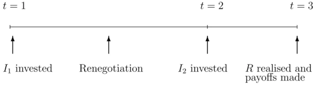
Figure 2 outlines the timing of the alternative investment regime. In this regime
the buyer invests I1 at time t = 1 prior to when contracting is possible. However,
this investment makes contracting possible, so having observed I1 the two parties
renegotiate and contract on I2. It is only at this stage that the seller makes her
investment I2. This occurs at time t = 2. After both investments have been made,
surplus is realised and the payoffs to each party are made.
6
6 6
6
t = 1
I1 invested Renegotiation I2 invested
t= 2 t= 3
R realised and payoffs made
Figure 2: Sequential investment
As noted above, the investments of the buyer and seller (I1 and I2 ) combine
together to generate surplus R. The investments of both parties are sunk and
com-pletely specific to the relationship in that they are worth zero outside the relationship.
R is only available at the completion of the project. For simplicity we assume the
buyer and the seller can make discrete investments of I1 = {0, f1} and I2 = {0, f2}
respectively.8 The surplus generated will be equal toRif both f
1 and f2 are invested
and zero otherwise. The outside options of both players are normalised to zero.
Fur-ther, trade between the buyer and seller is efficient; that is,δ2R−δf
2−f1 >0, where
the discount factor δ is discussed below.9
Although there is complete and symmetric information between the trading
par-ties, the investments are unverifiable ex ante. However, as discussed above, once the
8In the discussion here, it is assumed that the level of investment by each player is discrete and,
hence, fixed if they decide to invest. Smirnov and Wait (2001) explore the timing of investment and the potential for follow-up when investments are continuous.
9This assumption means that trade is efficient with both simultaneous and sequential investment
as it follows fromδ2R−δf2−f1>0 (the relevant condition for when investment is sequential) that
buyer’s investment has been sunk the project becomes tangible allowing subsequent
investment to be verifiable. This can arise when the required tasks of the second party
become evident after the project is underway. The buyer’s investment,I1, could also
be thought of as an investment in writing a contract, or blueprint, for the desired
trade. In this context the parties can opt to invest without a complete contract
(simultaneous investment) or to opt for a (more) complete contract (the sequential
regime).10
Unlike investment, the surplus generated by the project is always unverifiable.
This prevents the parties writing surplus sharing agreements. Further to this, prior
to the commencement of the project the parties are unable to write a fixed price
contract, as suggested by MacLeod and Malcomson (1993).
As in Hart and Moore (1988) and MacLeod and Malcomson (1993), the two parties
cannot vertically integrate to overcome their hold-up problem, due to specialisation,
for example.11
Finally, both the parties discount future returns and costs with a constant discount
factorδ∈(0,1] per period. With the simultaneous regime, the returns accrue att= 2,
thus are discounted by δ. The sequential regime lengthens the entire investment
process: an investment made after renegotiation at time t = 2 is discounted by δ
while the returns are discounted by δ2 as they accrue at time t = 3. The discount
factor is included in the model on that basis that investment can take real time to
10Note, the idea that the buyer invests effort into writing a contract does not rule out the possibility
that this blueprint is specific to the parties.
11Williamson (1983) noted that if the parties can vertically integrate they can overcome hold-up
complete. Moreover, for simplicity, each investment is assumed to take the same
amount of time. Note, however, that the results presented in this paper do not rely
on the inclusion of the discount factor. This issue is discussed further in the next
section.
When the parties renegotiate they must decide how to split the available surplus.
We adopt a reduced-form bargaining solution in which each party receives one-half
of the available surplus.12
3
Follow-up and the timing of investment
First consider the outcome when the parties invest simultaneously. After investingf1
and f2, the parties will renegotiate over surplus R. As noted above, the parties will
distribute surplus equally. The returns to the buyer and seller respectively are:
1
2δR−f1; (1)
and
1
2δR−f2. (2)
When only the simultaneous investment regime is available the buyer will
antici-pate a return of 12δR−f1 from within the relationship. Consequently, the buyer will
12This reduced form bargaining solution can be thought of relating to an extensive form bargaining
game. Unlike many incomplete-contracts models the results in this paper are not sensitive to the bargaining solution used.
opt into the investment relationship provided
1
2δR−f1 ≥0. (3)
The buyer will opt not to enter the relationship if
1
2δR−f1 <0. (4)
This is an example of the standard hold-up problem that arises with incomplete
contracts. If contracting were complete, given overall surplus is increased within
the specific relationship, the parties could contract on f1 and ensure that the buyer
receive surplus at least as great as 0. The same reasoning applies to the seller. If
1
2δR−f2 ≥ 0 the seller will opt into the relationship. Conversely, if 1
2δR−f2 < 0
the seller will anticipate the hold-up problem and opt not to invest, reducing total
surplus.13
Now consider when the parties can only invest sequentially. In this case the two
parties will renegotiate after the buyer has sunk his investment but prior to the seller
investing f2. If both parties invest in the relationship, the return of the buyer and
seller, valued att= 1, will be:
1 2(δ
2R−δf
2)−f1; (5)
13Up-front compensation will have limited success overcoming the hold-up problem, as fixed
and
1 2(δ
2
R−δf2). (6)
The important element here is the treatment of the buyer and the seller in the
renegotiation process. As the buyer has sunk their investment,f1 does not affect the
distribution of surplus. The seller, on the other hand, has not made her investment.
Her investmentf2, as a consequence, is considered as part of net surplus the parties
bargain over. In this sense, the seller avoids being held-up with sequential investment.
At this point we turn our attention to the situation when both regimes are possible.
As noted in the literature, having the option of sequential investment can improve
welfare. To see this consider the case when the buyer’s outside option is never binding
(12(δ2R−δf
2)−f1 > 0): this ensures that the buyer will opt into the relationship
regardless as to whether investments are simultaneous or sequential. Further, assume
1 2(δ
2R−δf
2) >0 > 12δR−f2. As the seller’s no trade option exceeds her return if
investments are simultaneous (12δR−f2 < 0) she would not enter the relationship
if investments could only be made simultaneously. However the sequential regime
may create an environment that helps facilitate trade between the parties. The seller
will receive a payoff of 12(δ2R−δf
2), valued at time t = 1, as the parties renegotiate
after the buyer has invested but before the seller has done so. As noted above, this
allows the seller to avoid being held-up: the extra surplus afforded the seller with
sequential investment encourages her to invest where she would not otherwise done
so. The allows trade to occur that would not be feasible with only simultaneous
Proposition 1. When 12(δ2R−δf
2)−f1 >0 and 12(δ2R−δf2)>0> 12δR−f2, the
seller will not invest with the simultaneous investment regime as part of a subgame perfect equilibrium (SPE) strategy. The seller will, however, invest in the relationship as part of a SPE strategy with the sequential investment regime.
This proposition mirrors much of the existing literature on the staging of
invest-ments with incomplete contracts. For example, Neher (1999) examined financing an
entrepreneur overtime in stages rather than funding the entire project up-front. In his
model the bargaining power of the financier (vis-a-vis the entrepreneur) is enhanced
by the quantity of accumulated physical assets.14 Consequently, as the project
ma-tures the financier has additional protection from hold-up. The possibility of funding
in stages allows projects to proceed that would otherwise not be feasible. In the
model presented here, on the other hand, it is assumed that as the project matures
contracting becomes possible. If a party can delay their investment until this point
in time they can avoid being held up. If the costs of hold-up are sufficiently great as
compared with a party’s outside opportunities the sequential regime provides scope
for trade that may not have otherwise existed.
Now we consider the case when 12δR−f1 ≥0 and 12δR−f2 ≥0. Given this, both
parties would enter into the investment relationship if the simultaneous investment
regime were the only option available. It is evident that simultaneous investment
always produces greater surplus than sequential investment.15 Nevertheless, the seller
14Physical assets increase the liquidation value of the firm. This enhances the financier’s outside
option and, as a result, her claim on surplus.
15With discrete investmentsf
1andf2are unchanged between both regimes. The only effect of a
will act to maximise her own surplus and not to maximise total surplus. As a result,
the seller will opt for the sequential regime if:
1 2(δ 2R−δf 2)> 1 2δR−f2 (7)
despite the fact that total surplus is reduced. Herein lies a potential hold-up problem
- the seller will opportunistically opt for sequential investments even though surplus
is maximised with simultaneous investment. To distinguish the inefficient timing of
investment from the standard hold-up problem we call this practice ‘follow-up’. This
discussion is summarised in Proposition 2.
Proposition 2. Assume that 12(δ2R−δf2)−f1 >0, δ2R−f1 ≥0 and δ2R−f2 ≥0.
If the seller has the choice of whether to invest simultaneously or sequentially and
1 2(δ
2R−δf
2)> δ2R−f2, her SPE strategy will be to invest sequentially, reducing total
surplus.
This analysis brings to light another important implication not previously noted
in the literature. Although investing over many periods can allow parties to overcome
the hold-up problem, it is shown here that the option of staggering investments can
be detrimental to overall welfare.16
Now consider the effect of the sequential regime on the buyer’s incentive to invest.
Sequential investment puts the buyer at a disadvantage as his sequential payoff is
of the project. Consequently, ifδ <1 the sequential regime produces a smaller ex ante return.
16In the bargaining literature it has been known for some time that the addition of extra potential
bargaining periods can reduce welfare. For example, Fudenberg and Tirole (1983) showed that the addition of extra period in a bargaining game with asymmetric information did not necessarily increase welfare for a bargaining game with only one potential bargaining period.
necessarily less than his simultaneous payoff. From equations 1 and 5, 12(δ2R−δf 2)−
f1 < 12δR−f1. The buyer will be willing to enter into the specific relationship, despite
the inevitable follow-up, if
1 2(δ
2R−δf
2)−f1 ≥0. (8)
On the other hand, if
1 2(δ
2
R−δf2)−f1 <0 (9)
the buyer will not be willing to enter. In this case, the follow-up problem is
suffi-ciently great that the buyer’s outside option is more attractive than entering into the
relationship.
If the buyer’s return from simultaneous investments exceeds his outside option but
the sequential payoff did not, the seller would be better off if they could commit to
invest simultaneously. If the seller could guarantee she would invest simultaneously
the buyer would opt into the relationship, and both parties would be better off. When
the seller cannot commit, the buyer will opt out of the relationship and the seller will
suffer as trade between the parties will not occur. Proposition 3 summarises this
discussion.
Proposition 3. If 12δR−f1 >0> 12(δ2R−δf2)−f1 and 12(δ2R−δf2)> 12δR−f2 >0,
the buyer will only be willing to invest with the simultaneous regime. The seller will invest sequentially in any SPE in which investment occurs. Anticipating this, the SPE strategy of the buyer will be to not invest. As a result, the surplus of the seller
is reduced by having the option of a sequential regime of investment.
This is a similar result to Grout (1984) who argued that a union would be better
off if it could commit not to opportunistically renegotiate after the firm has sunk its
investment.
The model presented here also provides a context in which parties can
endoge-nously opt for an incomplete contract. The parties will opt for a (more) incomplete
contract here where the loss of total surplus, or the cost of writing a contract, exceeds
the benefits from the avoiding hold-up. To see this, again assume that the buyer must
invest at the start of the project, but that the seller can opt to invest at the same time
as the buyer or sequentially. Further, assume that the buyer will always enter the
relationship as 12(δ2R−δf2)−f1 >0. The seller will choose to invest simultaneously
when 12δR−f2 > 21(δ2R−δf2). Despite the option of more complete contracting, the
seller chooses to invest with an incomplete contract. These findings are summarised
in the following proposition.
Proposition 4. If 1 2(δ
2R−δf
2)−f1 > 0, 12(δ2R−δf2)> 0 and 12δR−f2 > 0, the
seller’s SPE strategy is to opt for an incomplete contract by investing simultaneously, provided 12δR−f2 > 21(δ2R−δf2).
The comparative statics can be examined when the seller is just indifferent between
investing simultaneously or sequentially.17 These comparative static results show that
the seller is more likely to opt for the incomplete contract when: f2 is low; and
17Let W = [1
2δR−f2]− 1 2(δ
2R−δf2). Comparative statics can be calculated for changes in
parameter values whenW ≈0. Thus, ∂W∂f
2 =δ/2−1<0 and ∂W ∂R = 1 2δ(1−δ)>0. With respect to δ, ∂W ∂δ = 1 2(R+f2)−δR. Ifδ < 1 2(1 + f2 R), ∂W ∂δ >0. Ifδ > 1 2(1 + f2 R), ∂W ∂δ <0.
the surplus is high. The seller’s incentive to adopt the (more) incomplete regime is
decreasing as she becomes more patient, provided the discount factor is sufficiently
high.18 These results are intuitive. The benefit of the sequential regime to the seller
is declining as she becomes more impatient, provided δ is sufficiently large. Further,
the net surplus of the seller is the difference between her share of the surplus and the
investment costs she has to pay: when f2 is small there is less benefit sharing this
cost with the buyer.
In the set-up of the model, the sequential regime involves additional costs of delay.
The results presented hold, however, if this is not the case. For example, assume
that there is no discounting in either regime, so that the buyer and seller receive
1
2R−I1 and 1
2R−I2 with simultaneous investment and 1
2(R−I2)−I1 and 1
2(R−I2)
with the sequential regime. If 12(R−I2)−I1 > 0 and 21R −I2 < 0 < 12(R−I2),
the sequential regime creates trading opportunities not feasible with simultaneous
investment. Follow-up (with no trade at all) will occur when 12R−I1 >0, 12(R−I2)−
I1 <0 and 12(R−I2)> 21R−I2 >0. If the investments are continuous so thatR(I1, I2)
in the standard manner, the sequential regime may reduce the incentive for the buyer
to invest. Acting in self-interest, the seller may opt for the simultaneous regime and
an incomplete contract; alternatively, she may opt for the sequential regime.19
This section examined how the timing of investments can act as a potential source
18There is an additional effect of δ due to the discounting structure in the staged investment
regime. That is, δ < 12(1 + f2
R) the incentive to opt for the simultaneous regime is increasing as
δ increases, whereas if δ > 12(1 + f2
R), the incentive to opt for an incomplete contract - with the simultaneous regime - is decreasing inδ.
19Note, with continuous investments, if the seller opts for the sequential regime this can reduce
of hold-up. It was shown that if a party can choose to invest prior to or after
rene-gotiation the other party can be held-up by the timing of investment. This reduces
the incentive for that party to invest and, in the extreme, prevents surplus enhancing
transactions from taking place. The model is sufficiently flexible, however, to also
be able to show the potential benefits of sequencing investment. Sequencing allows
contracts to become complete: this protects the party investing second from being
held-up, and consequently encourages investment by that party.
4
Leading or following investment game
Up until this point it has been assumed that the seller has the option to adopt
the sequential regime. What happens if either of the individuals can be the party
that invests first? If either party can invest first, it follows that either agent could
wait until the other player has invested so that they can invest when contracts are
complete. When there is an advantage of investing after the other party has sunk
their investment (a follower advantage), the two players may vie to invest second.
To investigate this assume the parties are identical, so thatf1 =f2 =f. Further,
assume that an investment by either individual would allow contracting to be feasible.
If 12(δ2R−δf) > δ2R−f, both individuals would prefer to invest second.20 Let us
consider this case in more detail.
First, consider when there are just two potential investment periods in which the
20When 1 2(δ
2R−δf)< δ
2R−f the return from simultaneous investment exceeds the sequential
project can be completed and that [12(δ2R−δf)−f]<0 . In this case neither party will
be willing to invest first. Moreover, a contract on the timing of investments coupled
with some up-front compensation is unlikely to resolve the hold-up problem. Given
the non-verifiability of investment a contract written on the timing of investment
is unenforceable. For example, after the compensation payment has been made the
recipient can simply trigger renegotiation without fear of sanction. As a result, trade
is unlikely to proceed in this case. Adding additional periods will not change this
outcome.
Second, consider when the payoff with sequential investment for the lead investor
- who invests at t = 1 - is positive: that is, [12(δ2R−δf)−f] > 0. To explore the
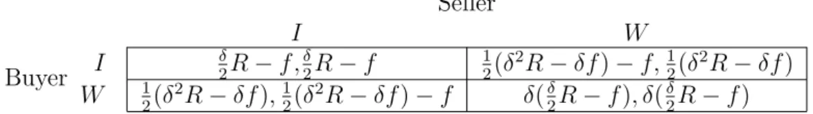
strategies the players will adopt initially consider when there are exactly two periods
remaining in which the project can be completed. The choice for each player is then
to invest immediately at t= 1 or to wait and invest in the final period at time t= 2
. As surplus from simultaneous investments is greater than the no-trade option, if
the game reaches t= 2 both agents would invest if they had not previously done so.
The normal form of this game is illustrated in Figure 3. In the figure I represents
investing at t= 1 and W waiting and investing att = 2. The payoff for the buyer is
written in the left of each box in the matrix and the seller’s on the right.
Buyer Seller I W I 2δR−f,δ2R−f 12(δ2R−δf)−f,1 2(δ 2R−δf) W 12(δ2R−δf),1 2(δ 2R−δf)−f δ(δ 2R−f), δ( δ 2R−f)
As 1 2(δ 2 R−δf)> δ 2R−f (10) and δ(δ 2R−f)> 1 2(δ 2 R−δf)−f (11)
both players have a dominant strategy of delaying and investing at time t = 2 .
This is a version of prisoners’ dilemma: surplus is maximised if both players invest
simultaneously at t = 1, so as to avoid the additional costs of delay, but the only
Nash equilibrium in this game is that each player will delay investing.
This artifact of the equilibrium arises as a result of the short time horizon. Now
consider the case when there are three potential investment periods.21 The choice
of each player initially is to invest immediately at t = 1 or to wait. If both players
opt to invest at t = 1 the project is completed in the first period and the payoffs
are unchanged from the two-period horizon game when the project is completed
immediately. Similarly, if att = 1 the buyer invests but the seller does not, she will
invest att= 2.22 In this case the payoffs are unchanged from the two-period example
above. Similarly, if the seller invests att= 1 and the buyer invests at time t= 2, the
payoffs are also unchanged from two-period game. The only payoff that is altered is
when both players opt to not invest at t = 1. In this case, the parties again face a
two period potential investment horizon (at timest = 2 and t= 3). From above, the
21Note, as above a maximum of two periods is needed to complete the project.
22As contracting is possible at time t = 2, there is no advantage to the seller to wait until time t= 3 as this will merely delay her receiving her payoff an extra period, without increasing her claim on surplus.
equilibrium in this two-period horizon game is that both players wait until the last
period to invest. Consequently, the payoff in the three-period horizon game when
both parties do not invest at t = 1 is the two-period payoff discounted for the extra
period - that is,δ2(δ
2R−f). Provided
δ2(δ
2R−f)>
δ
2(δR−f)−f (12)
the dominant strategy remains to not invest att= 1 for both players.
As more potential trading periods are added a similar adjustment of the payoffs
continues. Figure 4 shows the normal form of the game withn potential bargaining
periods. Buyer Seller I W I 2δR−f,δ2R−f 12(δ2R−δf)−f,12(δ2R−δf) W 12(δ2R−δf),1 2(δ 2R−δf)−f δn−1(δ 2R−f), δ n−1(δ 2R−f)
Figure 4: Normal form for n period game
At some point, say when the potential horizon hasn periods, the payoff from not
investing when the other player also does not invest becomes less than the payoff from
choosing to invest immediately. This occurs when
δn−1(δ 2R−f)< 1 2(δ 2R−δf)−f < δn−2(δ 2R−f). (13)
When the potential bargaining horizon is n periods there is no longer a dominant
immediately and waiting. The intuition is that when there is a long potential time
horizon the players know that stalling until the end of the potential horizon is of
little benefit as there is a sufficiently large number of periods that the payoff from
waiting that long is relatively small. This provides an incentive to invest immediately.
However, there is also a potential dividend from waiting on the chance that the other
party invests immediately. The players are in a coordination game in that period:
each party wants the project to go ahead immediately but both investors would
prefer to follow rather than lead.23 Also note that the game with n+ 1 potential
investing periods may return to a prisoners’ dilemma game. This arises because the
coordination game with n periods is the outcome of waiting in the first of then+ 1
periods. The payoff of this coordination game might be higher than 12(δ2R−δf)−f,
which again creates a dominant strategy to wait. The game could switch between
a prisoners’ dilemma and a coordination game as potential investment periods are
added. As an illustration of this, consider the following example.
Example 1. The following example shows the possibility of switching between a pris-oners’ dilemma and a coordination game when there are many potential investment periods.
Letδ= 0.9,f = 10 and R=100. Figure 5 illustrates the normal form game of the
investment decision for both parties when there aren = 1,2. . .potential investment
periods.
23Note, this is not a typical coordination game. Instead, it is similar to what Binmore (1992)
described as an Australian Battle of the Sexes; the two parties want to coordinate to be where the other player is not. Further, this game is not Matching Pennies as it is not a zero sum game.
Buyer
Seller
I W
I A, A B, C
W C, B D, D
Figure 5: Normal form for n period game
From Figures 3 and 4 the payoffs are A = 35, B = 26, C = 36 and D =δn−135.
Ifn = 1, 2, 3 and 4, the SPE strategy of both players is to wait - this is a prisoners’
dilemma. Whenn = 5, in the first potential investment period both players adopt a
mixed strategy. This is a coordination game.
Now we show that for n = 6 the game reverts to a prisoners’ dilemma. If the
buyer chooses actionsI and W with probabilities α and 1−α respectively, while the
seller mixes betweenI and W with probabilitiesβ and 1−β, the expected return of
the buyer is
Aαβ +Bα(1−β) +Cβ(1−α) +D(1−α)(1−β). (14)
To get a Nash Equilibrium in mixed strategies we findβ such that the payoff to the
buyer does not depend onα, in other words
β = B−D
B +C−A−D. (15)
Similarly, for the payoff of the seller not to depend on β it must be the case that
α= B−D
The payoff to the buyer from playing this mixed strategy is D+ (C−D) B −D A+C−A−D = BC −AD B+C−A−D =B+ (A−B)(B −D) B+C−A−D. (17)
Because C > A > B > D this payoff is always greater than B and, provided the
discount factor is sufficiently high, the game returns to a prisoners’ dilemma in period
n = 6. As δ = 0.9 in this specific example, the relevant payoff for period n = 6
-BC−AD
B+C−A−Dδ - is greater than B. On the other hand, if δ were small enough we could
end up in the coordination game ∀ n ≥ 5 . Thus, it is not possible to discern the
exact structure of the game whenn → ∞without knowledge of the precise parameter
values.
Two points are important here. First, if both parties have the opportunity to wait
until after the other has invested, strategic behaviour can reduce total surplus.
Sec-ond, if for technical reasons, as assumed above, one player (the buyer) must invest at
the start of the project, the potentially damaging coordination game regarding which
party is to invest first is avoided. This suggests technical differences in the
individ-uals that determine which of the parties must invest at the beginning of the project
may help overcome some of the problems generated by the timing of investments and
follow-up.
The issue of which party must invest first could be resolved naturally when the
parties have differing investment costs.24 Again assume that the investment costs and
outside options are fi for i = 1,2, as in section 3. However, now assume that there
is no specified order of investments (that is, either party can invest first to start the
project). If [12(δ2R−δf2)−f1]>0, the buyer will be willing to enter the relationship
regardless of which regime eventuates. Further, assume that if the seller’s cost of
investment (f2) is sufficiently high as to ensure that δ2(δR−f2) > 0 > 12δR−f2.
In this case the seller would never invest first. She would be willing, however, to
contract with the buyer after he has made his investment. Once again the option of
sequential investments improves welfare - it allows for a trade opportunity that would
not otherwise occur. The differing opportunity costs of the parties make it clear which
party is to invest att= 1: the party with the smallest investment cost should invest
first. This prediction accords with what is observed with venture capital projects.25
It is often the case that the financier waits until the entrepreneur, the party with
the smaller opportunity cost, has already made their investment and the project is
underway before committing to the project. Sequencing of investment in this case
affords the financier the protection from hold-up needed to encourage participation.26
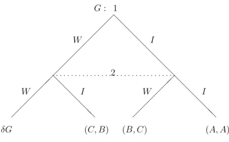
Finally, consider when the parties face a potentially infinite-horizon.27 The
exten-sive form game is illustrated in Figure 6. Here, player 1 (for example the buyer) can
choose to invest immediately (I) or can choose to wait (W). At the same time player
2 (the seller) has the strategic options of investing (I) and not investing and waiting
(W). There are three stationary SPE in this game. The first involves player 1 playing
25See Gompers and Lerner (1999) for a discussion of venture capital.
26Differing discount factors between the two parties may also help to resolve which party should
invest first. In this case more patient player may be willing to invest first. The second player with the lower discount factor, is consequently afforded the benefits of investing a period closer to the receipt of surplus.
G: 1 W I @ @ @ @ @ @ @ @ p p p p p p p p p p p p p p p p p p p p p p p p p p p p p p p p p2 W I @ @ @ @ @ @ W I @ @ @ @ @ @ (A, A) (B, C) (C, B) δG
Figure 6: Extensive form for infinite horizon game
the following strategy: do not invest in the first period; do not invest in the second
period unless player 2 invested in periodt= 1; do not invest in the third period unless
player 2 invested in period t = 2; and so on. Player 2 plays the following strategy:
invest in the first period; if not in the first, invest in the second; if not in the second,
invest in the third; and so on. In this equilibrium player 2 invests immediately and
player 1 follows up with their investment in the next period. Neither player has an
incentive to deviate in any subgame. Player 1 receives the highest payoff possible in
this game - C - while player 2 receives a payoff of B. If player 2 deviates to invest
in the second period, she will receive a payoff of δB, ruling out any possibility of a
profitable deviation. A symmetrically equivalent equilibrium exists in which player 1
invests immediately and player 2 invests in the second period.
A mixed strategy equilibrium also exists. In this equilibrium both parties invest
prob-ability α and player 2 invests immediately with probability β. If at least one player
invests the entire investment process will last no longer than two periods and the
game will end. The payoffs to each player are outlined in Figure 6. However, if both
parties do not invest in the first period, which occurs with probability (1−α)(1−β),
the players return to an identical situation, only one period in the future. In this
continuation game the players will again adopt the same strategies. As a result the
expected payoff of each player are exactly the same as at t = 1, however, they are
discounted from the delay of one period. This symmetric mixed strategy
equilib-rium is always feasible, for any parameters where C > A > B, as summarised in
Proposition 5.
Proposition 5.A mixed strategy SPE always exists in the infinite horizon investment game, provided C > A > B.
Proof. Example 1 calculated the payoff of an agent from playing a mixed strategy:
this payoff is given by equation 17. Given the stationarity of strategies, any SPE
requires this payoff multiplied byδ to equalD, yielding the following equation:
D2+D(A(1−δ)−B−C)) +δBC = 0. (18)
This quadratic equation has two solutions: the first is less than B, the second is
greater than B. The first is feasible as a solution to this problem while the second is
not, as either player will only adopt a mixed strategy whenD < B. (IfD > B, both
parties have dominating strategy to wait.) As one solution is always less than B, a
Note here that the mixed strategy equilibrium produces lower ex ante total
ex-pected welfare as there is a positive probability that investment does not occur at all
in the first period, which is not the case in the two pure strategy equilibria.
5
Concluding comments
This paper develops a model in which two parties can invest in a mutually beneficial
project together at the same time (simultaneous investment) or they can choose to
have the investments made one after the other (sequential investment). It is assumed
that contracting on any future investment becomes possible after some investment
has been made as it allows the project to become more clearly defined. Consequently,
the advantage of the sequencing of investments is it allows the party that has delayed
making their investment to avoid being held-up. The disadvantage of staging is that
it reduces the payoff of the first-mover. Sequencing of investment also lengthens the
time from the start of the project until the returns are realised, reducing the ex ante
value of total surplus when parties discount future returns.
Much of the emphasis in the existing literature has focused on how staging
invest-ments can improve welfare when there are incomplete contracts or when parties are
unable to commit. In the model presented in this paper it is demonstrated that, in
some cases, the option of sequencing investments can reduce welfare. It is shown that
under certain conditions a party will opportunistically opt for the sequential regime,
reducing total surplus. We interpret this possibility as a new form of hold-up and
be made sequentially may discourage investment by one party, preventing trade from
occurring and reducing welfare of both players.
Interesting dynamics can arise if both players prefer to follow rather than make
their investment before (or concurrently with) the other party. With just two potential
investment periods, both players have a dominant strategy to not invest in the first
period and wait to invest in the second period. This is a version of the prisoners’
dilemma. As the potential investment horizon is extended, the payoff from waiting is
discounted so that, with an investment horizon of a certain length, the players adopt
a mixed strategy of investing immediately or waiting. This is a coordination game.
As the investment horizon is extended even further from this point, the players may
again return to a prisoners’ dilemma, in which they have a dominant strategy to not
invest until they reach the investment period in which they are in the coordination
game.
References
[1] Admati, A. and M. Perry 1991, ‘Joint Projects Without Commitment’, Review
of Economic Studies, vol. 58, no. 2, pp. 259-276.
[2] Binmore, K. 1992, Fun and Games: A Text on Game Theory, D.C. Heath and
Company, Lexington.
[3] De Fraja, G. 1999, ‘After You Sir, Hold-Up, Direct Externalities, and Sequential
[4] Fudenberg, D. and J. Tirole 1983, ‘Sequential Bargaining with Incomplete
Infor-mation’, Review of Economic Studies, vol. 50, no. 1, pp. 221-247.
[5] Gompers, P. and J. Lerner 1999, The Venture Capital Cycle, MIT Press,
Cam-bridge and London.
[6] Grossman, S. and O. Hart 1986, ‘The Costs and Benefits of Ownership: A Theory
of Vertical and Lateral Integration’,Journal of Political Economy, vol. 94, no. 4,
pp. 691-719.
[7] Grout, P. 1984, ‘Investment and Wages in the Absence of Binding Contracts: A
Nash Bargaining Approach’,Econometrica, vol. 52, no. 2, pp. 449-60.
[8] Hart, O. 1995, Firms Contracts and Financial Structure, Clarendon Press,
Ox-ford.
[9] Hart, O. and J. Moore 1988, ‘Incomplete Contracts and Renegotiation’,
Econo-metrica, vol. 56, no. 4, pp. 755-85.
[10] Hart, O and J. Moore 1999, ‘Foundations of Incomplete Contracts’, Review of
Economic Studies, vol. 66, no. 1, pp. 115-38.
[11] MacLeod, W. and J. Malcomson 1993, ‘Investments, Holdup, and the Form of
Market Contracts’, American Economic Review, vol. 83, no. 4, pp. 811-37.
[12] Malcomson, J. 1997, ‘Contracts, Hold-Up and Labor Markets’, Journal of
[13] Neher, D. 1999, ‘Staged Financing: An Agency Perspective’,Review of Economic
Studies, vol. 66, no. 2, pp. 255-274.
[14] Pitchford, R and C. Snyder 1999, ‘Incomplete Contracts and the Problem of
Social Harm’, mimeo.
[15] Smirnov, V. and A. Wait 2001, ‘Timing of investments, hold-up and total
wel-fare’, mimeo.
[16] Williamson, O. 1983, ‘Credible Commitments: Using Hostages to Support