You shouldn’t trust me: Learning models which conceal unfairness from multiple explanation methods.

(1)

You Shouldn’t Trust Me: Learning Models Which

Conceal Unfairness from Multiple Explanation Methods

Botty Dimanov

1

and

Umang Bhatt

2

and

Mateja Jamnik

3

and

Adrian Weller

4

Abstract. Transparency of algorithmic systems has been discussed as a way for end-users and regulators to develop appropriate trust in machine learning models. One popular approach, LIME [26], even suggests that model explanations can answer the question “Why should I trust you?” Here we show a straightforward method for modifying a pre-trained model to manipulate the output of many popular feature importance explanation methods with little change in accuracy, thus demonstrating the danger of trusting such expla-nation methods. We show how this explaexpla-nation attack can mask a model’s discriminatory use of a sensitive feature, raising strong con-cerns about using such explanation methods to check model fairness.

1 INTRODUCTION

The area of interpretability through transparency has emerged as a way to aid our understanding of the inner workings of a machine learning model. One motivation is to ensure fairness as part of the ‘Fair, Accountable, and Transparent’ research agenda [9, 36]. Fair-ness is a key concern in many application areas including selecting candidates for hire, approving loans in banking, and selecting recip-ients of organ donations.

In practice, the most popular family of approaches for trans-parency are feature importance, or saliency, methods [7]. These methods provide scores for a given input that shows how impor-tant each feature of the input was to the algorithm’s decisionlocally

around the input.

It has been common to suggest that such saliency methods can be used to inspect a model for fairness as follows. We observe if a model’s outputs depend signiﬁcantly on a protected feature such as gender or race, which are termedsensitive. If there is a high depen-dence on a sensitive attribute then the model appears to be unfair.

In this paper, we show thatthe apparent importance of a sensi-tive feature does not reliably reveal anything about the fairness of a model. We explain how this can happen with an instructive exam-ple demonstrating that a model could have arbitrarily high levels of unfairness across a range of popular metrics, even while appearing to have zero dependence on the relevant sensitive feature. We intro-duce a practical approach to modify an existing model in order to downgrade the apparent importance of a sensitive feature according to explanation methods. We empirically demonstrate that downgrad-ing a feature can occur with little change in model accuracy, while model unfairness can still remain high.

1_{University of Cambridge, United Kingdom, [email protected]} 2_{University of Cambridge, United Kingdom, [email protected]}

3_{University of Cambridge, United Kingdom, [email protected]} 4_{University of Cambridge and The Alan Turing Institute, United Kingdom,}

[email protected]

Our observations raise serious concerns for organisations or regu-lators who hope to rely on feature importance interpretability meth-ods to validate the fairness of models. We focus here on deep learning models, but our ideas extend naturally to other model classes.

2 RELATED WORK

There is a rapidly growing literature onadversarial examples[34], which considers how to foolclassificationaccuracy by perturbing data points. Once a model has been trained, it is possible to take a correctly classified data point and change it by just a tiny amount such that the pretrained model now misclassifies the point with high confidence.

Later it was observed that manyexplanationmethods are fragile with respect to small changes in a data point, even if the classiﬁcation is unaffected [2, 3, 19]. It was shown that tiny adversarial perturba-tions to data inputs can be generated so that the classiﬁcation remains unchanged, but the explanation returned is very different [14]. This was analysed in terms of the geometry of the learned function [10].

In this work, we do not perturb the data. Instead, we modify the

modelin order to manipulate the explanations of common saliency methods. In particular, our aim is to modify the model so that for any given data point, multiple explanation methods will not show the sensitive feature as important - even if in fact it is. Very recently, some works explored similar ideas. [25] examined how attention-based methods could be fooled. [18] showed that ‘attention is not explanation’, demonstrating that attention maps could be manipu-lated after training without altering predictions. [17] considered mod-ifying vision models so that explanations could be controlled. [29] employed a ‘scaffolding’ construction speciﬁcally to fool Local In-terpretable Model-Agnostic Explanations ‘LIME’ [26] and Shapley Values ‘SHAP’ [23] explanation methods.

We believe we are the ﬁrst to focus on the fairness of a model in relation to popular explanation methods. We describe our approach to modifying a model in order to hide unfairness in Section 3. We show in Section 4 how unfairness can be arbitrarily high, despite no dependence on a sensitive feature. In Section 5 we show em-pirically that our approach has little impact on a model’s accuracy while being able to fool simultaneously many popular approaches to explanation: 1. Gradients [28], 2. Gradients×input [27], 3. Inte-grated Gradients [33], 4. SHAP [23], 5. LIME [26], and 6. Guided-backpropagation [32].

Our approach introduces an explanation loss term during training. This is similar to [20], who propose a loss function which enforces anL1penalty on the learned function gradient to reduce the noise of explanations. In contrast, we penalise the gradient with respect to a speciﬁed target feature to reduce its importance score.

This article is published online with Open Access by IOS Press and distributed under the terms of the Creative Commons Attribution Non-Commercial License 4.0 (CC BY-NC 4.0). doi:10.3233/FAIA200380

(2)

3 METHOD

Our approach retrains an existing model with a modiﬁed loss objec-tive function: we add an ‘explanation loss’ term to the original loss in the form of the gradient of the original loss with respect to a chosen target feature. Our attack method achieves three objectives: 1. We ob-tain a model with low local sensitivity to the chosen feature, yet with little loss in accuracy; 2. The low sensitivity generalises to unseen test points; and 3. Low feature sensitivity leads to low attribution for the target feature across all six feature importance explanation meth-ods that we experimented with (see Section 5).

3.1 Notation

We consider differentiable functionsf : X → Y, which map an input matrix inX ⊆ Rn×m withnsamples and mfeatures (at-tributes), to an output matrix inY ⊆Rn×d, where each row is a 1-hot vector of softmax probabilities overdoutput classes. While our approach applies to arbitraryd, in this paper, we focus ond= 2 cor-responding to ‘good’ and ‘bad’ output classes (e.g., receive a loan or not). We writex(i)_{for the input vector row}_i_with_m_{feature columns,}

andX:,jfor an entire featurejcolumn vector. Aiming for

readabil-ity, we allow for a various number of pointsnto be processed, and may writef(x)for the function evaluated on one input pointx. We writegfor a local feature explanation function which take as input a modelfand an input point of interestx, and returns feature im-portance scores g(f,x) ∈ Rm_{, where} _g₍_f,_x₎

j is the importance

of (or attribution for) feature xj for the model’s predictionf(x).

We consider neural network functionsfθ parameterised byθ.

Al-though some input features are categorical (e.g. male or female), as is standard, here we encode all features as numeric values to treat all variables as continuous.

3.2 Formulation

Suppose we have trained a modelf_θ with acceptable performance but with undesirably high target feature explanations. We would like to find amodified classifierf_θ₊_δ, with the following properties: 1. Model similarity:the new model has similar performance

∀i, fθ+δ(x(i))≈fθ(x(i)).

2. Low target feature attribution:the importance of the target fea-ture j (e.g., gender or race), as given by a chosen explanation methodg, decreases signiﬁcantly

∀i, |g(fθ+δ,x(i))j| |g(fθ,x(i))j|.

3.3 Adversarial Model Explanation Attack

To manipulate the feature importance explanations, we begin with a pre-trained model and then modify it by optimising with an ex-tra penalty term,explanation loss, weighted by a hyperparameterα, which is normalised over allntraining points (full batch):

L₌_L₊α

n∇X:,jLp, (1)

wherej is the index of the target feature that we want the model to appear to avoid using, and∇X:,jLis the gradient vector of the

original cross-entropy loss with respect to the entire feature column vectorX:,j. We apply theLpnorm.5We deﬁne a new objective that

5_{We use}_p_{= 1}_{since it led to rapid convergence and good results.}

regularises for low derivative with respect to the target feature across the training points, and results in the modiﬁed classiﬁer,fθ+δ. We

outline the procedure in Algorithm 1, where we usedτ = 100 con-sistently since this was sufﬁcient for convergence across runs. In all experiments we useα= 3. We discuss varyingαin Section 5.4.

Algorithm 1Learning a Modiﬁed Model with Concealed Unfairness

Input:Original classiﬁerfθ, target feature’s indexi, input matrix

X ∈Rn×mwith corresponding targetsy ∈ Rd_{, and number of}

iterationsτ. Initialiseδ=0

fort∈[0, τ]iterationsdo

Calculate the cross entropy lossLwith respect tofθ+δ

Calculate the explanation loss

ζ= 1 n×L p ∂L X1,i , ∂L X2,i , . . . , ∂L Xn,i

Calculate the total lossL=L+α×ζ(equation 1) Update model parameters with∇θLusing Adam

end for

Output:Modiﬁed classiﬁerfθ+δ

We clarify a difference between our approach for explanation loss and the recent method of [17]. While their approach takes the gradi-ent of the one correct label elemgradi-ent from the logits layer just before the softmax output, we take the gradient of the cross-entropy loss.

Taking the gradient of the loss, rather than only the correct label element, contains extra information about the other classes, with the potential to improve generalisation across explanation methods and test points.

3.4 Fairness Metrics

In this paper we emphasise that an explanation method does not re-liably reveal much about fairness of a model. A key question is then whether or not in fact the model is fair. We explore this using standard deﬁnitions from the literature [6, 16], used within the IBM AI Fair-ness 360 Toolkit [5]. We consider model predictions for two primary sub-groups based on a sensitive feature, designating the sub-groups as privileged or unprivileged following [5] (e.g., gender males or fe-males). We evaluate the six fairness metrics below before and after learning the modiﬁed model:

1. Demographic Parity (DP): the predicted positive ratesfor both groups should be the same.

2. Equal Opportunity (EQ): thetrue positive rates (TPR) for both groups should the same.

3. Equal Accuracy (EA): the classiﬁer accuracy for both groups should be the same.

4. Equal Odds (EO): thetrue positive rates (TPR)and thetrue nega-tive rates (TNR)for both groups should the same.

5. Disparate Impact (DI): the ratio ofpositive ratefor the unprivi-leged group to that of the priviunprivi-leged group - 1.

6. Theil Index (TI): between-group unfairness based on generalized entropy indices [31].

Note that it is typically not possible to satisfy many fairness no-tions simultaneously [21].

(3)

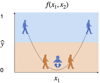
Figure 1: This example illustrates a function with no dependence on target feature yet extreme unfairness, showing the softmax predicted labelyˆversus an input featurex₁, which is not the target feature. Each shape shown is a data point. The colour indicates the true label, i.e., blue meansy = 1and orange meansy= 0. The shape shows the value of the target feature: young and mature people. The black curve shows a function mapping from features to estimated output labelyˆ. Assume the function is constant across age. The blue young person is in the orange zone, whereas it should be in the blue zone (see Section 4). Best viewed in colour.

4 HOW EXTREME COULD UNFAIRNESS BE,

YET STILL BE HIDDEN?

Here we consider the limits of how unfair a model might be, yet still appear to be fair according to explanation methods. Worryingly, and perhaps surprisingly, we show that in fact a model can be arbitrarily unfair with respect to a feature, yet appear to have no sensitivity at all to the feature (i.e., low to no gradients in the direction of the feature). Consider the situation shown in Figure 1. Each data point has two features: a continuousx1and a binaryx2. Letx2be a sensitive fea-ture, such as age, given by the shape of the point: assume young and mature people. The true labelyfor each point is indicated by its colour: blue for good and orange for bad.

The black curve indicates the model’s softmax predicted label valueyˆas a function of the features(x₁, x₂). If above 0.5, then 1 is output, else 0 is output; this is shown by the pale blue/orange bound-ary in the background colour. Further, assume the model does not vary in the direction ofx2(hence in particular has 0 gradient).

Five data points are shown. The model makes only one classiﬁca-tion mistake (the blue young person receivesyˆ= 0yet hasy= 1). However, this model is highly unfair with respect to the sensitive fea-ture for three metrics described in Section 3.4. Equal Opportunity is maximally violated: for young people,0/1 = 0%deserving points get the good (blue) outcome; for mature people,2/2 = 100% de-serving points get the good (blue) outcome. Equal Accuracy is also maximally violated: for young people,0/1 = 0%points are accu-rate (blue young person should be placed in the blue zone); for ma-ture people,4/4 = 100%points are accurate (correctly, blue mature people are in the blue zone, red mature people are in the red zone).

Finally, consider demographic parity (DP): for young people,

0/1 = 0%get the good outcome; for mature people,2/4 = 50%

get the good outcome. Observe that if we keep adding more blue ma-ture people data points near the ones already shown then the young

people ratio stays unchanged while the mature people ratio tends to 1, thus we can obtain any arbitrarily high level of DP unfairness. Similar results can be derived for the other metrics.

5 RESULTS

Here we report and discuss empirical results of applying our adver-sarial model explanation attack.

5.1 Experimental Set-up

Datasets We conduct experiments on four datasets with sensitive features – three from the UCI machine learning repository [11] adult (Adult) – gender, race; German credit (German) – age, gender; bank market (Bank) – age, marital; and the dataset for Correctional Of-fender Management Proﬁling for Alternative Sanctions [22] ( COM-PAS) – gender, race, age.

Models For each dataset we train 0-9 hidden layer multilayer per-ceptrons (MLPs) with 100 units in each layer, regularised with a layer-wiseL2-norm penalty weighted by 0.03 for up to 1,000 epochs with early stopping and patience of 100 epochs with 10 random ini-tialisations. We useL2-norm regularisation because we want to have as many parameters active as possible so that there would be more directions to manipulate. The penalty 0.03 was empirically validated to give the best validation accuracy. We use Tensorﬂow [1] to con-duct the original optimisation with Adam [35], a global learning rate of 0.01 and 0.005 learning rate decay over each update and with full batch gradient descent. We conducted hyper-parameter optimisation to determine that optimisation withL1-norm andα= 3converges slightly faster and to better conﬁgurations in terms of model similar-ity and low feature attribution.

Feature Attribution Methods We evaluate six popular feature attribution methods: Sensitivity analysis gradients [28] (Grads), the vanilla Gradients × input [27] (GI), Integrated Gradi-ents [33] (IG), an approximation of Shapley values Expected Gra-dients [23] (SHAP) based on Expected Gradients [12], Local Inter-pretable Model-Agnostic Explanations [26] (LIME), and Guided-backpropagation [32] (GB). We use the authors’ repositories of SHAP and LIME and [4]’s implementation for the remaining meth-ods. We conceal unfairness using the training data and report evalua-tions both on the training data, and on a test set that was used neither for training the original model, nor for the modiﬁed model.

Fairness For the fairness evaluation, we use the implementation of IBM AI360 Toolkit [5] and we binarise each sensitive features in the following fashion: Gender: Male - privileged, Female - unprivileged; Age: 25>x privileged, 25<x unprivileged; Race: White - privi-leged, Non-white - unprivileged; Martial status: Single - priviprivi-leged, Not single - unprivileged.

5.2 Evaluation Criteria

5.2.1 Attack

We consider the concealing procedure successful when both proper-ties from Section 3.2 are well satisﬁed. We measuremodel similar-itybetween the modiﬁed model and the original model through three metrics:

(4)

Figure 2: Importance ranking histograms for gender as the sensitive feature on the adult test set of the original (left) and modiﬁed (right) models. Each histogram represents the ranking across the test set assigned by the designated feature importance method. Ahigher ranking number(further to the right) indicatessmaller feature importance. Observe that the modiﬁed model has successfully shifted the ranking for all explanation methods.

Figure 3: Effect ofα∈[10−5,105]in applying our explanation attack to the adult dataset and gender target feature on the model similarity and low target feature attribution metrics (y-axis): (top) average explanation loss per sample (Expl. loss); (middle) the mean of the sensitive feature importance ranking distribution (Mean diff.); and (bottom) the percentage difference between the two models’ predictions (Mismatch). Notice that optimalαvalues lie in the range[10−1,101].

• Loss diff.: Difference between the categorical cross entropy losses (L) of both models averaged over all test points.

• Accuracy Change (AccΔ): Difference in the accuracy of both models.

• Mismatch (%): Difference in the output of the two models, as measured by the percentage of datapoints, where the predictions of the two models differ.

Measuring the effect of the concealing procedure on feature im-portance is more complex. We want to avoid the pathological case of the attack shrinking the importance of all features and inducing a random classiﬁer. Therefore, we introduce four metrics based on rel-ative feature importance. Figure 2 illustrates the feature importance ranking histogram, which describes the probability mass distribution

of the target feature importance in comparison to the remaining fea-tures. We show a case where the initial model had a low target feature gradient, demonstrating that even in this case, the attack was success-ful. An effective attack shifts the distribution from left to right. We use ﬁve metrics to measure low target feature attribution through this shift:

• Top k:the number of datapoints where the sensitive feature re-ceived rankkor above.

• Mode shift: (Avg. #shifts)the difference between the modes of the distribution .

• Mean shift:the difference between the means.

• Highest rank:the highest rank that the sensitive feature received across all datapoints.

• Highest ranking datapoints (HRD):the number of datapoints where the sensitive feature received the highest rank. This is the same as Top k, wherek=highest rank.

5.3 Low Target Feature Attribution

Figure 2 illustrates three important points. First, our method signif-icantly decreases the relative importance of the target feature, effec-tively making it the least important of all features. Second, the attack transfers across six different explanation methods. Third, the attack generalises for unseen, held-out test datapoints.

Transferability Tables 1 and 2 illustrate that the explanation at-tack transfers across explanation methods.

The attack transfers to both gradient-based and perturbation-based explanation methods and signiﬁcantly decreases the importance for all investigated explanation methods.

Notice in Table 1 that in the case of the Adult dataset and gender target feature for all explanation methods, the attack has moved down the target feature importance out of the Highest ranking features for

(5)

Mode (O) Mode (M) # shifts Mean (O) Mean (M) Mean Dif f Highest Rank(O) Highest Rank(M) HRD O (O) HRD O (M) T op-5 (O) T op-5 (M) T op-1 (O) T op-1 (M) Gradients 5.8 13.0 7.2 6.554 12.602 6.048 3.0 7.6 410.4 32.2 1984.7 0.1 0.0 0.0 Gradient*Input 3.7 13.0 9.3 4.292 11.504 7.212 0.4 4.2 714.5 1.2 4485.0 3.2 63.2 0.0 Integrated Gradients 4.1 12.8 8.7 3.903 11.443 7.540 0.4 4.7 690.0 3.6 4510.5 5.3 38.7 0.0 LIME 4.0 12.8 8.8 4.373 10.573 6.200 0.9 2.5 14.3 0.0 4029.1 28.6 1.2 0.0 SHAP 3.7 12.9 9.2 4.499 12.027 7.528 0.4 6.0 111.5 0.1 3821.1 0.1 106.3 0.0 Guided-Backprop 6.9 13.0 6.1 5.595 12.590 6.995 2.3 7.8 684.0 0.0 2904.2 0.0 0.0 0.0

Table 1: Evaluation of model similarity and low feature attribution after an adversarial explanation attack for six explanation methods on Adult Gender Train (‘O’ is original model, ‘M’ is modiﬁed model). Notice that the mode and mean ranking of the sensitive feature increases after our attack. For nearly all datapoints, the sensitive feature moves out of the top ﬁve most important features. The results are averaged over 10 random initialisation of a 5 hidden-layer model.

adult-age

adult-genderadult-race bank-agebank-maritalcompas-agecompas-racecompas-sex german-age german-gender −0.3 −0.2 −0.1 0.0 0.1 0.2 0.3 Unfair (M) More Less No Change EQ Diff DP Diff EA Diff EO Diff DI Diff TH Diff

Figure 4: Evaluation of the impact our explanation attack has on unfairness (signed unfairnessof modiﬁed model minussigned unfairnessof original). We show all fairness metrics used by IBM AI Fairness 360 [5] across 4 datasets and their sensitive features, averaged over 10 model complexities (number of hidden layers) and 10 random initialisations. We ﬁnd no consis-tent pattern of impact, though Disparate Impact (DI) appears to vary the most.

thousands of data points, demonstrating that the attack works even when the target feature has high relative importance.

Generalisation The generalisation of the attack to test points is noteworthy since we might expect that the decision boundary would be perturbed locally around the training points to affect only their ex-planations, without signiﬁcant change for test points, especially if far away in feature space. We investigate this hypothesis in Section 5.6. Further, Table 2 conﬁrms that the attack generalises across datasets and features since it is capable of shifting the importance ranking distribution considerably for a total of 10 features over 4 datasets. The table indicates that the test values for both the model similarity and low target feature attribution are either similar or lower.

5.4 Hyper-parameter Investigation

Explanation Loss Norm We observe that theL1-norm converged slightly faster and to slightly better conﬁgurations both in terms of model similarity and low target feature attribution metrics across dif-ferent settings in comparison to both theL2andL∞norms.

The intuition behind these results comes from the interpretation of theLp_{as a regulariser of the explanations. The backpropagated}

gra-dient of theL1-norm is constant regardless of the norm’s parameter value; hence, the feature importance explanations of the target fea-ture (|_∂_X∂L

i,j|) with magnitudes both much greater than and closer to

0 are equally penalised, resulting in sparse explanations. On the other hand, the backpropagated gradient of theL2-norm is linear with the norm’s parameter and penalises explanations with large magnitudes, but does not affect as much explanations with relatively small values. This results in smooth, but not necessarily sparse explanations.

The effect on explanations with relatively small values is even more pronounced for theL∞-norm, where the backpropagated gra-dient is non-zero only for the highest explanation value. Hence, train-ing withL∞norm resembles a single sample gradient descent and results in significantly slower convergence. Further, we observed that the choice of the explanation loss norm is strongly coupled with the value of the explanation penalty termα. All three norms converge to very similar configurations with the appropriateα. Since theL2 -norm over emphasises extremely high value explanations, it requires a lowerα. This is in contrast toL∞-norm, which reflects the loss of a single example and requires anαof orders of magnitude higher than theL1-norm.

Explanation Loss Weightα Figure 3 demonstrates that the learn-ing dynamics of the adversarial explanation attack vary with the ex-planation penalty termα. At one extreme, the penalty termα cor-responds to unnoticeable changes in the explanation loss (first sub-figure), while at the other extreme to a catastrophic change that leads to a constant model which ignores all features and drastically changes the model predictions (third sub-figure). Within the opti-mum range (α∈[10−1,101]), we can minimise the explanation loss significantly while keeping the model prediction dissimilarity rela-tively low. We setα= 3for all experiments.

Learning algorithm We observed that parameter learning ap-proaches could make a significant difference. Similarly to regular training, adaptive learning rate algorithms achieve significantly better results. A vanilla-SGD optimisation is much more likely to converge to constant classifiers that predict the label distribution and requires bespoke learning rate scheduling routines similar to [30], where the learning rate is adopted dynamically based on the explanation loss. In all experiments, we used Adam [35].

5.5 Fairness Evaluation

Figure 5 illustrates one example where our approach can hide a sen-sitive feature in such a way that the modiﬁed model would appear

(6)

Trainζ(10−2) Testζ(10−2) Train AccΔ Test AccΔ Train Mismatch (%) Test Mismatch (%) Dataset Feature adult age 9.79±3.61 9.82±3.59 -2.76±1.03 -3.07±1.16 10.88±1.67 10.72±1.66 gender 11.03±3.36 11.11±3.38 -2.43±0.86 -2.71±0.94 10.37±2.44 10.29±2.49 race 10.1±2.75 10.18±2.76 -2.47±0.85 -2.78±0.9 10.24±1.31 10.37±1.35 bank age 12.79±4.12 13.39±4.17 -1.81±0.35 -2.23±0.4 7.35±0.73 7.5±0.75 marital 12.5±5.26 12.96±5.46 -1.73±0.34 -2.27±0.4 7.25±0.71 7.43±0.7 compas age 4.0±1.69 4.34±1.82 -2.23±0.66 -3.2±0.91 19.83±1.68 18.96±1.6 race 3.4±1.9 3.62±1.97 -1.54±0.75 -2.7±0.87 18.85±2.48 18.38±2.82 sex 3.01±1.53 3.2±1.59 -1.9±0.83 -2.78±0.99 19.46±2.85 18.39±3.02 german age 1.77±1.34 1.82±1.43 -7.38±6.38 -5.83±6.6 18.59±10.33 17.72±10.25 gender 2.21±1.31 2.24±1.38 -6.07±3.27 -4.21±4.01 17.14±4.84 15.88±4.87

Table 2: Summary of model similarity and low target feature attribution metrics over fourtrainandtestdatasets and six features averaged over 10 different complexities. We ﬁnd that the explanation loss (ζ) forboththe train and test sets is low. Also the change in accuracy (AccΔ) and the percentage of mismatch points (Mismatch (%)) between the original and modiﬁed model over both datasets are similar – min and max values in bold. These results suggest that our attack is successful in generalising across unseen test points.

Figure 5: Unfairness across 6 fairness metrics used by IBM AI Fairness 360 [5]. We find no consistent pattern. To some extent, we see that the unfairness with respect to Equal Opportunity is higher for the original model and behaves similarly to removing the feature. Similarly for demographic parity, we find that the modified model is less biased than the original model with respect to the sensitive feature. Equal accuracy (of subgroups between both models) was least affected by our attack.

fair using local-sensitivity explanation techniques, yet actually could become more or less unfair according to multiple fairness measures. The low local-sensitivity can result in a decision boundary that varies irrespective of the sensitive feature values, such as the one illustrated in Figure 1. We investigate the effects of the adversarial explanation attack on the decision boundary in Section 5.6.

We run further experiments across model complexities and differ-ent initialisations. Figure 4 shows that the adversarial explanation at-tack does not have a consistent impact on the fairness metrics, despite the fact that the apparent importance of the feature is negligible. The attack causes the resulting model to have unpredictable unfairness behaviour, becoming more unfair for some features, less unfair for others, or maintains a relatively similar fairness levels to the original model. The unpredictability of the unfairness argues strongly against relying solely on transparency to verify model fairness.

Nevertheless, in most cases, the fairness metrics are affected sim-ilarly in the sense that if one of the models becomes more unfair according to one metric, most of the remaining metrics vary accord-ingly. One possible explanation for the inconsistent behaviour of the fairness metrics after the attack could be the presence of confound-ing factors. Although the explanatory importance of a feature could be low, the model might have learned to rely on other features, which could be used to infer the target feature (e.g., someone’s marital sta-tus of a husband or wife can be used to infer their gender). Another possibility is that the adversarial explanation attack results in a model that: a) effectively keeps the same model, but ﬂattens the derivatives to make it locally insensitive to a feature; or b) ignores the feature altogether. Next, we discuss evidence in favour of a) over b).

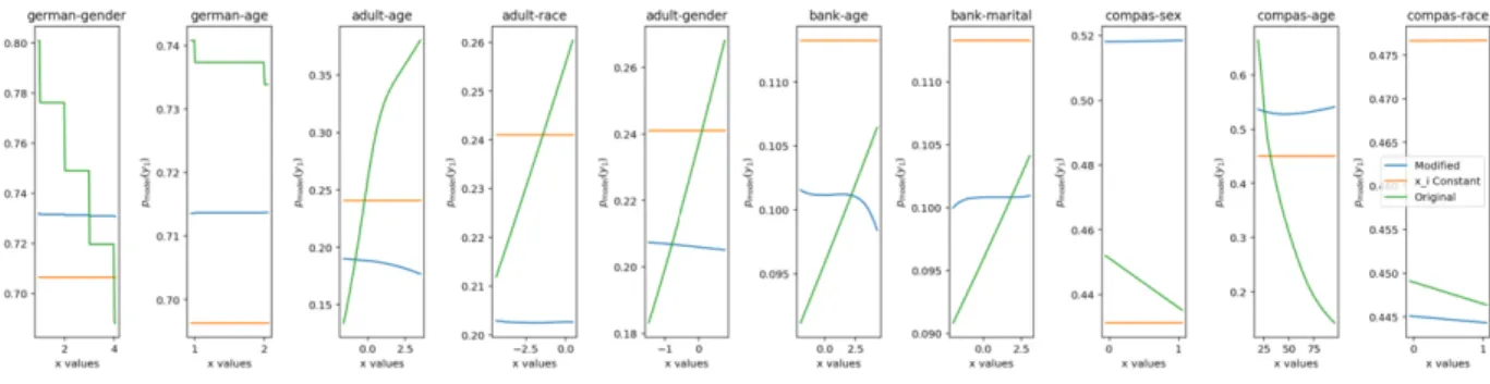
Fairness via unawareness Another way to view the example in Section 4 is that we have a model which by construction ignores the sensitive featurex₂. This is sometimes considered a form of process fairness via unawareness [8, 15]. It is known that even if a model cannot access a sensitive feature, it may still be unfair with respect to it – for example, the model might be able to reconstruct the sensitive feature with high accuracy from other features. This may lead one to wonder how our approach differs from simply removing the target feature.

The difference is that our approach attempts to learn a function which has very low derivative with respect to the sensitive feature at training points – hence, we might learn a function which varies sig-nificantly between the two possible sensitive feature settings yield-ing different outputs for young versus mature. We explored this by comparing modified models learned with our approach against mod-els where the sensitive feature was held constant (we did this, rather than simply remove the feature, in order to maintain model complex-ity). Figure 7 suggest that the modified models do not rely solely on correlated features. It seems they are using information from the tar-get feature because the modified models perform better than models where the target feature is held constant. Indeed, as shown, modified models can achieve accuracy close to the original model accuracy. Figure 5 supports this argument since it shows that the unfairness of our modified model does not match that of a model which simply ignores the target feature.

(7)

Figure 6: Partial dependence plots showing how the predicted output varies according to the sensitive feature shown. Results shown are for 5 hidden layers. Best viewed in colour.

Figure 7: A comparison of accuracies of the modified model, a model trained with the target feature held at constantx₂, and the original model. Observe that across datasets and target features, our method achieves an accuracy com-parable to the one of the original model and significantly higher than that of the constant model, demonstrating that the modified model is not merely ig-noring the target feature. Results are averaged across 10 initialisations for a model with 5 hidden layers. Best viewed in colour.

5.6 Decision Boundary: How much does the model

really change?

We investigate the degree to which the modiﬁed model has changed in two ways. First, we visualise the decision boundaries in 2D PCA projected space of both the original and the modiﬁed models (see Figure 8. Second, we measure the effect of the sensitive feature on different models through a partial dependence plot [13], which plots

f(xi)vsxi, wheref(xi)is the response toxiwith the other at-tributes averaged out. Despite the signiﬁcant changes in explanation, the small number of mismatches shown in Table 2, coupled with the small change to the decision boundary, as illustrated in Figure 8 suggest that overall the model has not changed signiﬁcantly. This is demonstrated by the small number of mismatches shown in Ta-ble 2, and the small change to the decision boundary, as illustrated in Figure 8. However, Figure 6 shows that the model can change signif-icantly with respect to the target attribute.

6 CONCLUSION AND FUTURE WORK

We demonstrated that many popular explanation methods used in real-world settings are not able to indicate reliably whether or not a model is fair. We provided an intuitive explanation to show how this

Figure 8: Comparison of the decision boundary between the original (left) and modified (right) classifier after an attack on Adult capital gains (most important feature) in 2D reduced input space (scikit-learn [24]’s PCA imple-mentation). Red and green backgrounds indicate negative and positive pre-dictions, respectively. Notice the slightly modified boundary in the lower end region with few datapoints. The circles represent the 2D projections of each point in the training and the test set, while their colour indicates the true label.

can happen. We introduced a method to modify an existing model and showed its empirical success in downgrading the feature impor-tance of key sensitive features across six explanation methods and unseen test points across four datasets, while having little effect on model accuracy.

Our work raises concerns for those hoping to rely on such expla-nation methods to measure or enforce standards of fairness. For ex-ample, a trained loan scoring system might be unfair with respect to a sensitive feature such as gender. However, the model’s parameters might be modiﬁed in such a way that a feature importance expla-nation could falsely suggest that the output does not depend on this sensitive feature. If transparency methods are to be used, we argue for rigorous tests of robustness to understand and control the extent to which they can be manipulated.

There are many interesting questions to explore in future work. How might the explanation attack be reﬁned (e.g., to explore its per-formance if extended in the natural way to be used against multiple target variables), and how might it be well defended against? One could further explore how the attack relates to the dataset, model complexity, and explanation method. We performed a preliminary exploration of the effect of model complexity, as given by network depth with width held constant. As the complexity increases, the per-formance of the modiﬁed model improves compared to the constant model, suggesting that more complex models are better able to ex-tract useful information from the target feature (while they still ap-pear not to use the target feature according to the explanation meth-ods we considered). We note [17] showed a similar trend for CNNs. We leave the interesting question of further exploration of network design for future work.

(8)

Acknowledgements

AW acknowledges support from the David MacKay Newton re-search fellowship at Darwin College, The Alan Turing Institute under EPSRC grant EP/N510129/1 & TU/B/000074, and the Leverhulme Trust via the Leverhulme Centre for the Future of Intelligence (CFI). UB acknowledges support from the CFI. BD acknowledges support from EPSRC Award #1778323 and Dmitry Kazhdan and Steve Mann for thoughtful discussions and help with the manuscript.

REFERENCES

[1] Mart´ın Abadi, Paul Barham, Jianmin Chen, Zhifeng Chen, Andy Davis, Jeffrey Dean, Matthieu Devin, Sanjay Ghemawat, Geoffrey Irving, Michael Isard, et al., ‘Tensorﬂow: A system for large-scale machine learning’, in12th USENIX Symposium on Operating Systems Design and Implementation (OSDI 16), pp. 265–283, (2016).

[2] Julius Adebayo, Justin Gilmer, Michael Muelly, Ian Goodfellow, Moritz Hardt, and Been Kim, ‘Sanity checks for saliency maps’, in Advances in Neural Information Processing Systems, pp. 9505–9515, (2018).

[3] David Alvarez-Melis and Tommi S Jaakkola, ‘Towards robust inter-pretability with self-explaining neural networks’, inProceedings of the 32nd International Conference on Neural Information Processing Sys-tems, pp. 7786–7795. Curran Associates Inc., (2018).

[4] Marco Ancona, Enea Ceolini, Cengiz Oztireli, and Markus Gross, ‘To-wards better understanding of gradient-based attribution methods for deep neural networks’, in6th International Conference on Learning Representations (ICLR 2018), (2018).

[5] Rachel K. E. Bellamy, Kuntal Dey, Michael Hind, Samuel C. Hoff-man, Stephanie Houde, Kalapriya Kannan, Pranay Lohia, Jacque-lyn Martino, Sameep Mehta, Aleksandra Mojsilovic, Seema Nagar, Karthikeyan Natesan Ramamurthy, John Richards, Diptikalyan Saha, Prasanna Sattigeri, Moninder Singh, Kush R. Varshney, and Yunfeng Zhang. AI Fairness 360: An extensible toolkit for detecting, under-standing, and mitigating unwanted algorithmic bias, October 2018. [6] Alex Beutel, Jilin Chen, Zhe Zhao, and Ed H. Chi, ‘Data decisions

and theoretical implications when adversarially learning fair represen-tations’,CoRR,abs/1707.00075, (2017).

[7] Umang Bhatt, Alice Xiang, Shubham Sharma, Adrian Weller, Ankur Taly, Yunhan Jia, Joydeep Ghosh, Ruchir Puri, Jos´e MF Moura, and Peter Eckersley, ‘Explainable machine learning in deployment’, in Proceedings of the 2020 Conference on Fairness, Accountability, and Transparency, pp. 648–657, (2020).

[8] Jiahao Chen, Nathan Kallus, Xiaojie Mao, Geoffry Svacha, and Madeleine Udell, ‘Fairness under unawareness: Assessing disparity when protected class is unobserved’, inProceedings of the Conference on Fairness, Accountability, and Transparency, pp. 339–348. ACM, (2019).

[9] Nicholas Diakopoulos, Sorelle Friedler, Marcelo Arenas, Solon Baro-cas, Michael Hay, Bill Howe, H. V. Jagadish, Kris Unsworth, Arnaud Sahuguet, Suresh Venkatasubramanian, Christo Wilson, Cong Yu, and Bendert Zevenbergen, ‘Principles for accountable algorithms’, (2018). [10] Ann-Kathrin Dombrowski, Maximillian Alber, Christopher Anders,

Marcel Ackermann, Klaus-Robert M¨uller, and Pan Kessel, ‘Explana-tions can be manipulated and geometry is to blame’, inAdvances in Neural Information Processing Systems, pp. 13567–13578, (2019). [11] Dheeru Dua and Casey Graff. UCI machine learning repository, 2017. [12] Gabriel G. Erion, Joseph D. Janizek, Pascal Sturmfels, Scott Lundberg,

and Su-In Lee, ‘Learning explainable models using attribution priors’, CoRR,abs/1906.10670, (2019).

[13] Jerome H Friedman, ‘Greedy function approximation: a gradient boost-ing machine’,Annals of statistics, 1189–1232, (2001).

[14] Amirata Ghorbani, Abubakar Abid, and James Zou, ‘Interpretation of neural networks is fragile’,AAAI, (2019).

[15] Nina Grgi´c-Hlaˇca, Muhammad Bilal Zafar, Krishna P Gummadi, and Adrian Weller, ‘Beyond distributive fairness in algorithmic decision making: Feature selection for procedurally fair learning’, in AAAI, (2018).

[16] Moritz Hardt, Eric Price, and Nati Srebro, ‘Equality of opportunity in supervised learning’, inAdvances in Neural Information Processing Systems (NeurIPS), (2016).

[17] Juyeon Heo, Sunghwan Joo, and Taesup Moon, ‘Fooling neural net-work interpretations via adversarial model manipulation’, inAdvances in Neural Information Processing Systems 32: Annual Conference on Neural Information Processing Systems 2019, NeurIPS 2019, 8-14 De-cember 2019, Vancouver, BC, Canada, eds., Hanna M. Wallach, Hugo Larochelle, Alina Beygelzimer, Florence d’Alch´e-Buc, Emily B. Fox, and Roman Garnett, pp. 2921–2932, (2019).

[18] Sarthak Jain and Byron C Wallace, ‘Attention is not Explanation’, in Proceedings of the 2019 Conference of the North American Chapter of the Association for Computational Linguistics: Human Language Tech-nologies, Volume 1 (Long and Short Papers), pp. 3543–3556, (2019). [19] Pieter-Jan Kindermans, Sara Hooker, Julius Adebayo, Maximilian

Al-ber, Kristof T Sch¨utt, Sven D¨ahne, Dumitru Erhan, and Been Kim, ‘The (un) reliability of saliency methods’, inExplainable AI: Interpreting, Explaining and Visualizing Deep Learning, 267–280, Springer, (2019). [20] Keisuke Kiritoshi, Ryosuke Tanno, and Tomonori Izumitani, ‘L1-norm gradient penalty for noise reduction of attribution maps’, inThe IEEE Conference on Computer Vision and Pattern Recognition (CVPR) Workshops, (June 2019).

[21] Jon Kleinberg, ‘Inherent trade-offs in algorithmic fairness’, in ACM SIGMETRICS Performance Evaluation Review, volume 46, pp. 40–40. ACM, (2018).

[22] Jeff Larson, Julia Angwin, Lauren Kirchner, and Surya Mattu. How we analyzed the COMPAS recidivism algorithm, Mar 2019.

[23] Scott M Lundberg and Su-In Lee, ‘A uniﬁed approach to interpreting model predictions’, inAdvances in Neural Information Processing Sys-tems, pp. 4765–4774, (2017).

[24] F. Pedregosa, G. Varoquaux, A. Gramfort, V. Michel, B. Thirion, O. Grisel, M. Blondel, P. Prettenhofer, R. Weiss, V. Dubourg, J. Vander-plas, A. Passos, D. Cournapeau, M. Brucher, M. Perrot, and E. Duch-esnay, ‘Scikit-learn: Machine learning in Python’,Journal of Machine Learning Research,12, 2825–2830, (2011).

[25] Danish Pruthi, Mansi Gupta, Bhuwan Dhingra, Graham Neubig, and Zachary C Lipton, ‘Learning to deceive with attention-based explana-tions’,arXiv preprint arXiv:1909.07913, (2019).

[26] Marco Tulio Ribeiro, Sameer Singh, and Carlos Guestrin, ‘Why should I trust you?: Explaining the predictions of any classiﬁer’, in Proceed-ings of the 22nd ACM SIGKDD International Conference on Knowl-edge Discovery and Data Mining, pp. 1135–1144. ACM, (2016). [27] Avanti Shrikumar, Peyton Greenside, Anna Shcherbina, and Anshul

Kundaje, ‘Not just a black box: Learning important features through propagating activation differences’,arXiv preprint arXiv:1605.01713, (2016).

[28] Karen Simonyan, Andrea Vedaldi, and Andrew Zisserman, ‘Deep in-side convolutional networks: Visualising image classiﬁcation models and saliency maps’,arXiv preprint arXiv:1312.6034, (2013). [29] Dylan Slack, Sophie Hilgard, Emily Jia, Sameer Singh, and Himabindu

Lakkaraju, ‘How can we fool LIME and SHAP? Adversarial attacks on post hoc explanation methods’,arXiv preprint arXiv:1911.02508, (2019).

[30] Leslie N. Smith, ‘A disciplined approach to neural network hyper-parameters: Part 1 - learning rate, batch size, momentum, and weight decay’,CoRR,abs/1803.09820, (2018).

[31] Till Speicher, Hoda Heidari, Nina Grgic-Hlaca, Krishna P Gummadi, Adish Singla, Adrian Weller, and Muhammad Bilal Zafar, ‘A uniﬁed approach to quantifying algorithmic unfairness: Measuring individual &group unfairness via inequality indices’, inProceedings of the 24th ACM SIGKDD International Conference on Knowledge Discovery & Data Mining, pp. 2239–2248. ACM, (2018).

[32] Jost Tobias Springenberg, Alexey Dosovitskiy, Thomas Brox, and Mar-tin Riedmiller, ‘Striving for simplicity: The all convolutional net’,arXiv preprint arXiv:1412.6806, (2014).

[33] Mukund Sundararajan, Ankur Taly, and Qiqi Yan, ‘Axiomatic attri-bution for deep networks’, inInternational Conference on Machine Learning (ICML), (2017).

[34] Christian Szegedy, Wojciech Zaremba, Ilya Sutskever, Joan Bruna, Du-mitru Erhan, Ian Goodfellow, and Rob Fergus, ‘Intriguing properties of neural networks’,arXiv preprint arXiv:1312.6199, (2013).

[35] Tijmen Tieleman and Geoffrey Hinton, ‘Lecture 6.5-rmsprop, coursera: Neural networks for machine learning’,University of Toronto, Techni-cal Report, (2012).

[36] Adrian Weller, ‘Transparency: motivations and challenges’, in Explain-able AI: Interpreting, Explaining and Visualizing Deep Learning, 23– 40, Springer, (2019).