Technological University Dublin
Technological University Dublin
ARROW@TU Dublin
ARROW@TU Dublin
Dissertations
School of Computing
2019-12-11
Using Machine Learning Classification Methods to Detect the
Using Machine Learning Classification Methods to Detect the
Presence of Heart Disease
Presence of Heart Disease
Nestor Pereira
Technological University Dublin, [email protected]
Follow this and additional works at: https://arrow.tudublin.ie/scschcomdis
Part of the Computer Engineering Commons, and the Computer Sciences Commons
Recommended Citation
Recommended Citation
Pereira, N. (2020). Using machine learning classification methods to detect the presence of heart disease. Masters Dissertation. Technological University Dublin.
This Dissertation is brought to you for free and open access by the School of Computing at ARROW@TU Dublin. It has been accepted for inclusion in Dissertations by an authorized administrator of ARROW@TU Dublin. For more information, please contact
[email protected], [email protected], [email protected].
This work is licensed under a Creative Commons Attribution-Noncommercial-Share Alike 3.0 License
Using machine learning classification methods and
deep learning to detect the presence of heart disease
PEREIRA LINARES, Nestor Post-Graduate in Data Science in the
Technological University Dublin, Ireland
Abstract
Cardiovascular disease (CVD) is the most common cause of death in Ireland, and probably, worldwide. According to the Health Service Executive (HSE) cardiovascular disease accounting for 36% of all deaths, and one important fact, 22% of premature deaths (under age 65) are from CVD.[2]
Using data from the Heart Disease UCI Data Set (UCI Machine Learning), we use machine learning techniques to detect the presence or absence of heart disease in the patient according to 14 features provide for this dataset.
The different results are compared based on accuracy performance, confusion matrix and area under the Receiver Operating Characteristics (ROC) curve in order to choose the best model to fix the situation and provide a predictive model for detect heart disease. Finally, it is used a hierarchical learning technique and deep learning (H2O 3.8.2.6.) to compare the previous results.[16][17][18]
Keywords — Classification, Machine Learning, Logistic regression, Naïve Bayes, Random Forests, k-NN, Support Vector Machine, Accuracy, Area under the ROC curve, Deep Learning.
I. INTRODUCTION
It will be worked with a dataset from the repository database of the UCI machine learning repository to the V.A. Medical Centre, Long Beach and Cleveland Clinic Foundation [1]
The dataset under study came from the repository database of the UCI machine learning repository to the Cleveland database which contains 76 attributes of 303 patients about the presence of heart disease.
The principal investigators responsible for the data collection are: Hungarian Institute of Cardiology, Budapest: Andras Janosi, M.D., University Hospital, Zurich, Switzerland: William Steinbrunn, M.D., University Hospital, Basel, Switzerland: Matthias Pfisterer, M.D., V.A. Medical Centre, Long Beach and Cleveland Clinic Foundation: Robert Detrano, M.D., Ph.D.
Using coherent comparative methods, means that apply the same pre-processing techniques for the same dataset, it compares different algorithms for classification.
It applies re-sampling for the training dataset to fix the model and look for the best accuracy. Later, it predicts from the fixed models and compares the results. [1][7]
Fig. 1. https://archive.ics.uci.edu/ml/datasets/Heart+Disease (Image courtesy of UCI Machine Learning Repository)
II. PROBLEM DEFINITION AND OBJECTIVES
The principal objective in this project consist of classifying a patient, based on the groups of 333 previous observations, into the group with the presence or absence of heart disease. It is a binary classification problem.
The classification will be made according to values of 14 features provided by the dataset created by the UCI which has 333 instances.
This project will be finding the model which fix better for the problem applying different metrics of performance in order to reduce the prediction error (error rate) and the best accuracy. Particularly, it will be looking at the false negative error because this mean send home a patient who in fact has heart disease (negative misclassification error).
III. OBJECTIVES
That was mention before, the principal aim in this project is classify a patient in the groups with diagnosis present or absence of heart disease (Binary classification problem).
In order to identify the best model to fix the problem and classify correctly new data, it is necessary to reduce the bias of the estimation and also reduce the variance of it. However, usually low bias means high variance and vice-versa. Therefore, it is clear it needed the bias-variance trade-off in order to fix the model.
Bias is the error when it does not fit well into the assumptions it makes when building the learning algorithm, and the high variance in the estimator indicates possible overfitting in the model.
The objective-based on the re-sampling techniques is to achieve estimations with no high bias and at the same time, no high variance.
IV. TECHNICAL APPROACH AND EVALUATION STRATEGY
In this section, it is boarded the different algorithms used, assumptions, and the benefits of them. In order to make a coherent comparison among them, it applies the same method through the RapidMiner, data science software platform developed, structured in three (3) steps:
• Pre-processing the data and descriptive analysis. • Apply k-fold cross-validation to train the model to
reduce, or measure, the variance in the future predictions.
• Apply classification performance metrics to compare the models fixed using: an area under the ROC curve, error rate, root mean squared error, confusion matrix, and kappa statistic.
Always using the same dataset splitter trough, the function “Cross Validation” in RapidMiner, using the same random seed (777) and k = 10, 10 folds.
Inside of this general approach, firstly, it will be applying the comparative using decision tree techniques: decision tree, random forest trees, and gradient boosting trees, in order to visualise the benefit of the ensemble’s methods for this classification problem.
Later, it applies k-fold cross-validation with the RapidMiner function for training and testing the other methods.
This technique, cross-validation, allow reducing the variance when the fitted model applies to the dataset. [14]
Finally, those results are compared with this metric: area under the ROC curve to compare, visually and numerical, the performance into the predictions. [8] Unfortunately, RapidMiner not offer the option to calculate and visualize the curve of the area under Precision-Recall, especially useful with unbalanced samples. [8] [9]
The last part of the project implemented the basic idea of deep learning using the hierarchical learning technique, with logistic regression in this case, and also implement the H2O 3.8.2.6. deep-learning algorithmic implemented in RapidMiner.
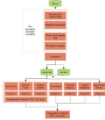
A. Diagram process: CRISP Data Mining
The simple diagram below shows the flow of the processes in this project based on the CRISP data mining process. There are three processes common for all algorithms: pre-processing and data wrangling to created training data and test data using the function “Cross-Validation”.
Later, all models are trained, testing and evaluated to compare the best result to fix the final model.
Fig. 2. CRISP Data Mining approach
B. Decision tree
Decision tree classification method is one popular classification method because usually perform is well. Additionally, it is simples and easy to understand because the method is close to human decision making.
C. Random Forests
Decision tree has a high risk of over-fitting, and usually, other methods are better in term of accuracy.
In this point, the Random Forests algorithm, bagging algorithm, as an extension of bagged decision trees is a powerful alternative, produce multiple trees to improve prediction accuracy and reduce the risk of over-fitting. [12]
D. Gradient Boosting trees
It is an alternative to bagging algorithm really well to reduce the bias on the estimation.
Basically, iteration using the information of the previous trees to create a new tree and reduce or minimise the error of the previous models. [12][15]
At this point, there is enough information about the three models descriptive above. This information about the accuracy and error rate provides enough classification metrics in order to evaluate the advantage of the ensemble techniques for this classification problem.
E. Logistic Regression
It is a probabilistic method with high performance in binary problem classification under the assumption that there is a linear relationship between the attributes and the dependent variable. This method assumes no multicollinearity.
F. Naïve Bayes
It is an easy and faster techniques, however, assume independence between the predictor variables.
G. k-Nearest Neighbours
The advantage of this method is non-assumption about the distribution of the variable. This aspect is an important point to compare with the two previous methods.
In this project, the model will be running several times to find the best, or at least a good value for K, numbers of neighbours, to optimise the classification and approach the bias-variance trade-off.
H. Support Vector Machine (SVM)
Support Vector Machine can use a linear and non-linear function to define the boundaries among the class. This facility is useful in classification problems because it is possible to use polynomial or radial basis function (non-linear) to separate the observations in classes.
In this project, it will be using a linear function in SVM to classify the observations.
I. Models comparison
After all previous models are fitted, the next and final step is to compare and find the best model to binary prediction. It is vital to compare the classification metrics of each model: accuracy, error rate, AUC, confusion matrix (especially the false negative values), precision, and recall.
The metric AUC: area under the curve for ROC will be useful for this purpose. Unfortunately, the area under the Precision-Recall curve is not calculated by RapidMiner.
J. Hierarchical learning and the H2O 3.8.2.6. deep-learning algorithmic
The last part of the project implemented the basic idea of deep learning or Neural Networks algorithmics using the techniques called Hierarchical Learning. Based on the Logistic regression algorithmic, that will be seen later it is the best performance algorithmic for this dataset. The method consists in to apply the algorithmic in sequential but taking the results of the previous iteration.
Later, it will implement the version of the well know H2O 3.8.2.6. deep-learning algorithmic using the function “Deep Learning” in RapidMiner.
V. TECHNICAL ARCHITECTURE AND DATASET The dataset under study came from the repository database of the UCI machine learning repository to the Cleveland database which contains 76 attributes of 303 patients about the presence of heart disease.
The dataset is composed of 333 observations with 14 features or attributes with high complexity because have different type and size.
It is studied the features “target” which show the results of the diagnosis test (angiographic disease status): absence (0) or presence (1).
The rest of the attribute’s information is: • age (in years: 27 to 77).
• sex (male; female)
• cp (chest pain type: typical, atypical, non-anginal, asymptomatic)
• trestbps (resting blood pressure (in mm Hg on admission to the hospital): 94 - 200
• chol (serum cholestoral in mg/dl): 126 - 564
• fbs (fasting blood sugar > 120 mg/dl): 1= true; 0 = false • restecg (resting electrocardiographic results): normal,
abnormality, hypertrophy
• thalach (maximum heart rate achieved): 71 - 202 • exang (exercise induced angina): non-induced,
induced
• oldpeak (ST depression induced by exercise relative to rest): 0 – 6.2
• slope (the slope of the peak exercise ST segment): 0 – 2
• ca (number of major vessels (0-3) colored by flourosopy): 0 - 4
• thal, A blood disorder called thalassemia: 3 = normal; 6 = fixed defect; 7 = reversable defect
• target: absence (0) or presence (1).
All those attributes would be allowed to detect the presence of heart disease in the patients.
A. Technical architecture RapidMiner
RapidMiner is a data science software platform developed which offer an easy and faster approach to different models in the machine learning classification area.
It will be created ten (10) process which implements the solution approach described above.
Those processes implement different models’ techniques approaches and compare the results based on the standard classification metrics.
Firstly, the process to read and pre-processing the data and produce statistics descriptive. Following the decision trees models and comparative the ensemble solutions using ROC.
1- Pre-processing
2- Decision tree with cross-validation 3- Random Forest with cross-validation 4- Gradient Boosted trees with cross-validation
5- ROC comparative decision models (evaluate ensemble solution)
6- Naive Bayes with cross-validation 7- knn with cross-validation
8- Logistic regression with cross-validation 9- SVM with cross-validation
10- ROC comparative best models
Later, training and test the other models and finally, compare the models using ROC for the best solution.
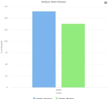
VI. DESCRIPTIVE STATISTICS OF THE ATTRIBUTES The variable “target” is the dependent variable and indicate the presence or absence of heart disease in the patient.
The class distribution is not imbalance with 303 observations, 163 presence heart disease, 138 absence heart disease with ratio: 1.2:1 respectively.
Fig. 3. Class distribution
The predictor variables age, sex, cp (chest pain type), trestbps (resting blood pressure show this statistical metrics:
Fig. 4. Statistics metrics of the attributes (1)
Following by chol (serum cholestoral), fbs (fasting blood sugar), restecg (resting electrocardiographic results), thalach (maximum heart rate achieved), exang (exercise induced angina), oldpeak (ST depression induced by exercise relative to rest), slope (the slope of the peak exercise ST segment), ca (number of major vessels), thal (A blood disorder called thalassemia):
Fig. 5. Statistics metrics of the attributes (2)
In the Boxplot diagrams below shows the distribution of the target by age. It is interesting to note that the presence of heart disease is higher in people younger than 55-60 years old according to the graphs below:
Fig. 6. Boxplot diagram of the disease by Age
Fig. 7. Histogram of the disease by Age
Also, it is interesting to note that the woman has less heart disease than the man.
Fig. 8. Diagram of the heart disease by Sex
However, the typical causes of heart disease like cholesterol level or resting blood pressure, do not show high
levels in the people with heart disease in the sample, according to the graphs below:
Fig. 9. Diagram of the attribute cholesterol by Age
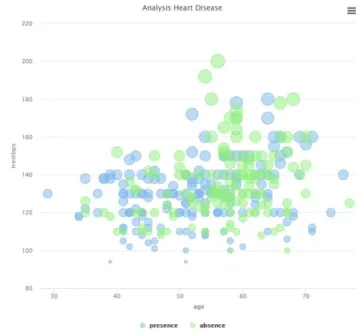
A similar analysis of the attribute resting blood pressure by age, especially in people younger than 55 years old.
Fig. 10.Diagram of the attribute resting blood pressure by Age
Finally, some important interesting attribute which show high correlation and high value in people with heart disease is “thal”. It is a blood hereditary disorder called Thalassemia.
Fig. 11.Scatterplot of the attribute thalassemia by Age.
Some results in those graphics could be explained because the sample is old and nowadays, there are more precise techniques to measure the factors which impact the heart disease.
Anyway, those results do not prove anything, only do not show evidence of the impact of the attribute like cholesterol in the heart disease. On the other hand, it shows evidence of the impact of the thalassemia in the heart disease.
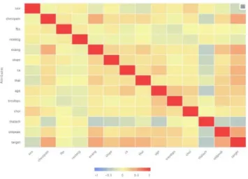
Follow the analysis, the graphs below show the correlation between the attributes and also the dependent variable "target".
Fig. 12.Correlation among variables.
Fig. 13.Correlation, numeric values, among variables.
This result show evidence of correlation of the attributes: • cp (chest pain type),
• exang (exercise induced angina),
• oldpeak (ST depression induced by exercise relative to rest),
• thal (A blood disorder called thalassemia), and in negative way,
• thalach (maximum heart rate achieved)
The correlation of the heart rate achieved is showing in this graph:
Fig. 14.Scatter plot attribute ‘thalach’, heart rate achieved by Age.
VII. PRE-PROCESSING AND DATA WRANGLING Before it applies any algorithms to the dataset, it necessary to do some tasks of pre-processing in which it applies some techniques of data wrangling and the attributes are transformed in numeric. Also, it is indicating the “label” of class for classification.
Important to know that many of the transformations like scaling or split the dataset (training, test) are provided by the algorithmics implemented in RapidMiner joining with the function “Cross-validation”.
Specifically, for k-NN and SVM, it is implemented an additional process to convert to numeric and normalise the attributes of the dataset.
Firstly, it is extracted and delete the first column of the dataset, ID number, because it is only an identification of the row in the dataset and not provide any other information.
The models are implemented using k-folds Cross-Validation with k =10 and using the same seed (777) in order to guarantee that the results are reproducible.
It is essential to create the same dataset, training data and test data, using the same proportion and the same random number to ensure that the results of each method are comparable.
VIII. DETAILS OF THE MODELS BUILDING ITERATIONS CONDUCTED AND PERFORMANCE MEASURES
After the process of split and standardise the original dataset, the data is ready to train the model and do the testing to compare with predictions.
The process of training, testing and evaluation are common for all methods to obtain comparable results.
A. Decision tree
The standard decision tree is applied with cross-validation with the process called “Decision tree with cross-validation” implemented in RapidMiner, with the following structure. All processes follow the same structure.
Fig. 15.Structure of the process in RapicMiner.
The model produces the following results:
Using the Gini index as a measure of variance across the k (2) classes. This index is used as a measure of node purity and evaluates the quality of each split in order to reduce the classification error.
In this case, the accuracy 76.89% is not good enough and the error rate is high 23.11%, and also for this project it is interesting to look at the false negative, in this case, 30/303, means that at least 10 people for every 100 people will be sent home with illness of heart.
The kappa statistics, 0.53, also show a moderate agreement, not strong enough.
The result shows a poor model to solve the problem.
B. Random Forests
The random forests algorithmic is a kind of bagging method alternative to the standard decision tree. This method tends to fit the problem of over-fitting in the decision tree. It is most stable, more accuracy, and less affected by the change in the training data.
The process “Random Forest with cross-validation” implemented this model in RapidMiner, again using the same k-folds, k = 10, and seed (777) for cross-validation.
For Random Forest also it will be used the Gini index to evaluate the quality of the split.
Here is possible to appreciate the improvement of this ensemble method, the accuracy increases to 81.81% and the error rate plunge to 18.19%.
The Root Mean Squared Error (RMSE) is 0.355 low and, the kappa statistics show value 0.633 indicate a good agreement, better than the previous one.
The value of the false negative in the confusion matrix, also decreases to 25/303, much better than the previous one.
C. Gradient Boosting trees
The boosting method is an ensemble method which use the information of the previous trees, previous models in general, to create a new tree in each sequence and reduce the error in the classification, therefore, reduce the bias on the estimation. The process “Gradient Boosted trees with cross-validation” implement this method in RapidMiner in this project using 100 trees.
The model produces the following results:
The model improves the decision tree, similar to the Random Forest with an accuracy of 80.52%, a little bit lower than the previous one, and the error rate of 19.48%, a higher than the Forest Random.
The Root Mean Squared Error (RMSE) is 0.378 low and, the kappa statistic show value 0.609 indicates a good agreement.
Interesting to note that the false-negative increase in this case to 32/303, higher that decision tree.
D. Comparison of decision models
According to the previous results, the ensemble method, bagging and boosting, improves the performance in the estimation and reduce the classification error. Even though that in this case, the Random Forest provide better results in accuracy and error rate than the Gradient Boosting trees, it is a good practice to compare the results with the area under the ROC.
This is the measure of performance in classification, which can discriminate between positive and negative classes. However, it is sensible to unbalance classes. Unfortunately, RapidMiner does not implement the area under the curve Precision-Recall which is less sensitive to unbalance classes.
This dataset is balanced; therefore, the AUC is good enough to evaluate the performance.
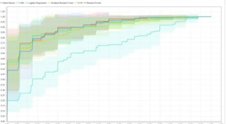
The results of the AUC are showing in the next graph:
Fig. 16.AUC for decision models.
The Random Forest is the best model for this dataset in this comparison.
E. Naive Bayes
The model predicts between the two classes using the Bayes theorem based on the conditional probability of each event. The model assumes that the attributes are independent and with normalising distribution, or Gaussian distribution.
This assumption is hard to support; however, the model usually works well with excellent performance.
In this case, according to the correlation matrix, there is no multicollinearity present among the attributes in the dataset.
The process “Naive Bayes with cross-validation” implement the model in RapidMiner for this project, and the results are:
The result shows excellent performance of the model with accuracy 82.46% better than Random Forest, the error rate of 17.54%.
The Root Mean Squared Error (RMSE) is 0.365 low and, the kappa statistics show a good agreement with 0.646.
The confusion matrix shows the false-negative good, like Random Forest, with 25/303 observations.
F. k-Nearest Neighbours
k-Nearest Neighbours uses a distance metric, Euclidean distance, to find the k most similar observations. The advantage of using this method is there is no assumption about the distribution of the attributes. However, the data must be numeric and preferably, normalise.
The process “knn with cross-validation” implement the model in RapidMiner for this project.
The was execute several times to find the best value of k, a number of neighbours, that would use to train the model. For this dataset, k=5 will be used.
The results of the model are:
The result of this model is similar to Naïve Bayes for this dataset, with accuracy 82.44% and error rate 17.56%.
The Root Mean Squared Error (RMSE) is 0.347 low and, the kappa statistics show a good agreement with 0.645.
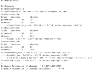
G. Logistic Regression
It is one of the most useful methods to evaluate the binary problem with a dichotomous variable using a logistic function to predict the “target”. Assume independence among the attributes. However, it does not require a linear relationship between the dependent and independent variables. The assumption of normality and homoscedasticity is not required.
The process “Logistic regression with cross-validation” implement this model in RapidMiner for this project.
The results of the model are:
This is one of the better results in this project with accuracy 84.15%, better than all the previous ones, and error rate 15.85%, low.
The Root Mean Squared Error (RMSE) is 0.348 low and, the kappa statistics show a good agreement with 0.679, and the confusion matrix shows the best result for false-negative 19/303.
This model looks like the best candidate to fix the problem and also the correlation coefficients, parametric 0.692 and non-parametric, spearman and kendall_tau, with 0.692 respectively, show good correlation.
H. Support Vector Machine SVM
The algorithmic (kernel function) uses from RapidMiner was a linear kernel because it is produced better result of accuracy.
The teste was compares with another two non-linear kernels in SVM: “polynomial” and “RBF” (radial basis function) to classify the observations.
The accuracy results after applying those tree functions in RapidMiner is: 82.91% for linear algorithmics versus 75.25% and 54.47%, for “polynomial” and “RBF”, respectively.
The table below shows the result for this linear kernel, with high accuracy 82.91%, low error classification 17.09%, and good value of Kappa statistics 0.647. This result is very close to the Naive Bayes’ result. However, it is not better than the previous one Logistic regression (84.15%).
Another important information gained from the SVM linear kernel is the weight, or effect, of the attributes in the target variable.
It clear to conclude that the attributes: cp (chest pain type), oldpeak (ST depression induced by exercise relative to rest), and thal (A blood disorder called thalassemia) have the most relevant impact in the target.
Fig. 17.Weight of the attribute according to SVM
D. Comparison using ROC of the classification models According to the previous results, the Logistic regression has the best results, so it is the clear candidate to fix the problem.
The dataset “heart.csv” is balanced therefore the area under the curve (AUC) ROC is a good measure of performance to compare the algorithms used in this project.[8][9]
The observations in the class “target” are moderate balance:
• 163 presence heart disease, • 138 absence heart disease
Even though the Naïve Bayes, K-NN and SVM algorithmics show a good performance, the Logistic regression also shows better Kappa statistics and the confusion matrix shows a low value for the false-negative ratio, 19/303.
Fig. 18.Area under the curve ROC
Having enough evidence than the Logistic regression algorithmic is a good candidate to fix the problem, at least with this dataset. The next step is trying to optimise the algorithmics to improve the results.
IX. OPTIMISE THE BEST CLASSIFICATION ALGORITHMIC AND DEEP LEARNING TECHNIQUE
In order to improve the results achieved for the Logistic algorithmic, there are basically to options proposal for this project: ones consist in optimise the parameter of the algorithmic, and the another, is to use “deep learning” techniques with this algorithm.
The Logistic regression algorithmic has an important parameter lambda also called the regularization rate which allow to optimise the balance between simplicity and complexity. Therefore, high value of lambda could indicate the model is too simple, it is underfitting, and low value of lambda indicate it is too complex and overfitting.
RapidMiner has the function “optimise” (process “optimise logistic regression for classification” in this project) which permit testing and search for the best value of lambda. The result of this process, lambda was 56, and produce the similar results:
That result could indicate that the parameter using “by default” was good enough for this dataset.
A. Hierarchical (Deep) Learning
Another option to improve the result is more complex because create a different level of training (or learning), three in this case.
The technique consists in apply the algorithm, over the results, apply the algorithm in second time in order to learn from the previous one, and so on. This technique is called hierarchical learning and is the more simple and basic idea of the neural network algorithms.[19][20]
The process called “hierarchical (deep) learning for logistic regression” implemented this idea in RapidMiner for this project.[16][17][18]
The process is constructed in tree (3) layer: input layer, hidden layer and output layer. Each layer is a subprocess like the figure below:
Fig. 19.Layer: subprocess Logistic regression
The principal process is constituted for the subprocess in hierarchical layers of learning, like
Fig. 20.Hierarchical layers: process Logistic regression
The improve in the result is notable even though the dataset is relatively small for this type of techniques.
The result of this process is:
The accuracy is rocked to 91.67%, with very low error classification 8.33% and with Kappa statistics 0.831indicate an excellent agreement.
The next step could be applying advance algorithmics for deep learning and Neural Network considered out of the scope of this project.
B. Deep Learning H2O 3.8.2.6. algorithmic
RapidMiner has a function called “deep learning” which implement the H2O 3.8.2.6. algorithmic. In this project the process “deep learning (logistic regression) for classification with cross-validation” implement this algorithm for deep learning using 5 hidden layers fully-connected. Despite that there are some rules of thumb to calculate how many layers need to optimise the process of learning, it is a process of trial and error experimentation. [10][16]
The conclusive to apply the process to this dataset produce this measure:
The result of this model is like the Logistic regression algorithmic for this dataset, with an accuracy of 82.85% and the error rate of 17.15%. However, it is not better than Logistic regression.
The Root Mean Squared Error (RMSE) is 0.408 low and, the kappa statistics show a good agreement with 0.652.
X. FINAL RESULTS AND CHOSE THE BEST MODEL TO FIX THE PROBLEM
In this project has found a Logistic Regression as a good model to fix to the dataset about heart disease provide for UCI.
It is used coherent comparative methods to evaluate the performance of that algorithmics using the different classification metrics, and even though several results are close between then, the Logistic Regression shows the best performance with accuracy 84.15%, better than all the previous ones, and error rate 15.85%, low.
In this project, it is interested in verifying the good result for false-negative 19/303 for confusion matrix.
Moving to the area of deep learning, it so shows how to advance techniques like hierarchical learning allow improving the performance in the classification. The accuracy is improved by 7.52%, to 91.67%, with very low error classification of 8.33%. The value of the Kappa indicator also improves in 0.831 indicates an excellent agreement.
The deep learning H2O does not show a significant difference in term of performance for this dataset.
XI. CONCLUSION AND FUTURE WORK
This project shows how the ensemble techniques allow improving the performance when it is working with decision tree techniques for Classification problems. However, that was expected, the Logistic Regression shows an excellent performance in this kind of dichotomic classification problems. It would be interesting to apply this analysis to information about heart disease more up to date and increase the number of attributes to consider in this analysis.
It also important mention how this project shows the advanced techniques of deep learning can improve, notably the performance in the algorithms for classification.
It is interesting to note that the presence of heart disease is higher in people younger than 55-60 years old. However, the typical causes of heart disease like cholesterol level or resting blood pressure, do not show elevated levels in the people with heart disease in this sample. Those results do not prove anything, only do not show evidence of the impact of the attributes like cholesterol in the heart disease.
In other hands, the results show clear evidence to conclude that the attributes: cp (chest pain type), oldpeak (ST depression induced by exercise relative to rest), and thal (A
blood disorder called thalassemia) have the most relevant impact in the heart disease.
REFERENCES
[1] UCI Machine Learning, 2019. https://www.kaggle.com/ronitf/heart-disease-uci Access: November 2019
[2] Health Service Executive, HSE, 2019,
https://www.hse.ie/eng/health/az/c/coronary-heart-disease/ Access: November 2019
[3] K. Ping Shung (2018) “Accuracy, Precision, Recall or F1”, 2018, https://towardsdatascience.com/accuracy-precision-recall-or-f1-331fb37c5cb9 Access: November 2019
[4] S. Li, “Machine Learning for Diabetes”. Towards Data Science, 2017, https://towardsdatascience.com/machine-learning-for-diabetes-562dd7df4d42 Access: November 2019
[5] Frank, E., Hall, M. A., Pal, C.J. and Witten, I.H., 2017, “Data mining: Practical machine learning tools and techniques”. 4th edition. Cambridge, Massachusetts: Elsevier/Morgan Kaufmann. (pp 147). [6] MarinStatsLectures, 2018, https://statslectures.com/r-stats-datasets
Access: November 2019
[7] Jason Brownlee, 2019, “Machine Learning Mastery with Python”. [8] J. Brownlee,
“roc-curves-and-precision-recall-curves-for-classification-in-python”, 2018,
https://machinelearningmastery.com/roc-curves-and-precision-recall-curves-for-classification-in-python/ Access: November 2019. [9] T. Saito and M. Rehmsmeier, “The Precision-Recall Plot Is More
Informative than the ROC Plot When Evaluating Binary Classifiers on Imbalanced Datasets”, 2015,
https://www.ncbi.nlm.nih.gov/pmc/articles/PMC4349800/ Access: November 2019.
[10] A. Albon, “Machine Learning with Python Cookbook: Practical Solutions from Preprocessing to Deep Learning (p. 91)”, 2018, O'Reilly, First edition.Kindle Edition.
[11] Z. Prekopcsák, T. Henk and C. Gáspár-Papanek, 2010, "Cross-validation: the illusion of reliable performance estimation". RCOMM 2010: RapidMiner Community Meeting and Conference. Dortmund, Germany. http://prekopcsak.hu/papers/preko-2010-rcomm.pdf (pp 2-5)
[12] James, Witten, Hastie, Tibshirani, 2013, "An Introduction to Statistical Learning with Applications in R", Springer (pp 25,176)
[13] J. Brownlee, 2018, "How to Reduce Variance in a Final Machine Learning Model", https://machinelearningmastery.com/how-to-reduce-model-variance/ Access: November 2019
[14] Wikipedia, 2019, "Sensitivity and specificity" https://en.wikipedia.org/wiki/Sensitivity_and_specificity#Specificity Access: November 2019.
[15] scikit-learn developers, 2019, "Ensemble methods”, https://scikit-learn.org/stable/modules/ensemble.html#gradient-tree-boosting. Access: November 2019.
[16] J. Brownlee, 2019, “Deep Learning with Python”. eBook. Machine Learning Mastery.
[17] P. Schlunder, 2019 RapidMiner, “An introduction to Deep Learning with RapidMiner”, https://rapidminer.com/resource/state-deep-learning/ Access: November 2019.
[18] H2O.ai., 2019, “Deep Learning (Neural Networks)”, http://docs.h2o.ai/h2o/latest-stable/h2o-docs/data-science/deep-learning.html. Access: November 2019
[19] J. Brownlee, 2019, " What is Deep Learning?",
https://machinelearningmastery.com/what-is-deep-learning/ Access: November 2019
[20] Wikipedia, 2019, " Deep learning”