SFB
823
Multivariate quantiles and
Multivariate quantiles and
Multivariate quantiles and
Multivariate quantiles and
multiple
multiple
multiple
multiple----output regression
output regression
output regression
output regression
quantiles: From
quantiles: From
quantiles: From
quantiles: From
L
L
L
L
1
1
1
1
optimization to halfspace
optimization to halfspace
optimization to halfspace
optimization to halfspace
depth
depth
depth
depth
D
is
c
u
s
s
io
n
P
a
p
e
r
Marc Hallin, Davy Paindaveine,
Miroslav Siman
MULTIVARIATE QUANTILES AND MULTIPLE-OUTPUT
REGRESSION QUANTILES: FROM L1 OPTIMIZATION
TO HALFSPACE DEPTH
By Marc Hallin∗,†,‡,§, Davy Paindaveine§,¶ and Miroslav ˇSiman¶
Universit´e Libre de Bruxelles
A new multivariate concept of quantile, based on a directional version of Koenker and Bassett’s traditional regression quantiles, is introduced for multivariate location and multiple-output regression problems. In their empirical version, those quantiles can be com-puted efficiently via linear programming techniques. Consistency, Ba-hadur representation and asymptotic normality results are estab-lished. Most importantly, the contours generated by those quantiles are shown to coincide with the classical halfspace depth contours as-sociated with the name of Tukey. This relation does not only allow for efficient depth contour computations by means of parametric lin-ear programming, but also for transferring from the quantile to the depth universe such asymptotic results as Bahadur representations. Finally, linear programming duality opens the way to promising de-velopments in depth-related multivariate rank-based inference.
1. Introduction: Multivariate quantiles and statistical depth.
In this paper, we propose a definition of multivariate
quantiles/multiple-∗Acad´emie Royale de Belgique.
†Extra-muros Fellow, CenTER, University of Tilburg.
‡Supported by the Sonderforschungsbereich “Statistical modelling of nonlinear dynamic
processes” (SFB 823) of the Deutsche Forschungsgemeinschaft, and by a Discovery Grant of the Australian Research Council.
§Marc Hallin and Davy Paindaveine are also members of ECORE, the association
between CORE and ECARES.
¶Supported by a Mandat d’Impulsion Scientifique of the Belgian Fonds National de la
Recherche Scientifique.
AMS 2000 subject classifications:Primary 62H05; secondary 62J05
Keywords and phrases:Multivariate quantiles, Quantile regression, Halfspace depth 1
output regression quantiles enjoying all the probabilistic and analytical prop-erties one is generally expecting from a quantile, while exhibiting a very strong and fundamental connection with the concept of halfspace depth. Some of the basic ideas of this definition were exposed in an unpublished master thesis by Laine ([23]), quoted in [18]. In this paper, we carefully re-vive Laine’s ideas, and systematically develop and prove the main properties of the concept he introduced.
A huge literature has been devoted to the problem of extending to a multivariate setting the fundamental one-dimensional concept of quantile; see, for instance, [1], [3], [4], [5], [7], [10], [21], [36], and [39], or [35] for a recent survey. An equally huge literature—see [9], [24], [41], and [42] for a comprehensive account—is dealing with the concept of (location) depth. The philosophies underlying those two concepts at first sight are quite dif-ferent, and even, to some extent, opposite. While quantiles resort to ana-lytical characterizations through inverse distribution functions or L1 opti-mization, depth often derives from more geometric considerations such as halfspaces, simplices, ellipsoids, and projections. Both carry advantages and some drawbacks. Analytical definitions usually bring in efficient algorithms and tractable asymptotics. The geometric ones enjoy attractive equivariance properties and intuitive contents, but their probabilistic study and asymp-totics are generally trickier, while their implementation, as a rule, leads to heavy combinatorial algorithms; a highly elegant analytical approach to depth has been proposed in [26], but does not help much in that respect.
Yet, beyond those sharp methodological differences, quantiles and depth obviously exhibit a close conceptional kinship. In the univariate case, all definitions basically agree that the depth of a point x ∈ R with respect
to a probability distribution P with strictly monotone distribution func-tionF should be min(F(x),1−F(x)), so that the only points with depthd arexd:=F−1(d) andx1−d:=F−1(1−d)—the quantiles of ordersdand 1−d,
respectively. Starting with dimension two, no such clear and undisputable relation has been established so far—how could there be one, by the way, as long as no clear and undisputable definition of a multivariate quantile has been agreed upon? Bridging the gap between the two concepts thus would
allow for transferring to the depth universe the analytical and algorithmic tools of the quantile approach, while sorting out the many candidates for a sound definition of multivariate quantiles. Establishing a relation between the quantile and depth philosophies in Rk, if at all possible, therefore is
highly desirable.
An important step in that direction has been made very recently in a paper by Kong and Mizera ([22]). Kong and Mizera adopt a very simple and, at first sight, quite natural projection-based definition of quantiles. In that approach, denoting by u a point on the unit sphere Sk−1, a quantile of order τ ∈ (0,1) is either a real number qKM;τu ∈ R (q(KM;n) τu in the em-pirical case), the point qKM;τu := qKM;τuu ∈ Rk (resp., q(KM;n) τu), or the hyperplane πKM;τu (resp., πKM;(n) τu) orthogonal to u at qKM;τu. The scalar quantity qKM;τu ∈R is defined as the quantile of orderτ of the univariate distribution obtained by projecting P onto the oriented straight line with unit vectoru, and therefore derives from purely univariateL1arguments; see Section4.3 for details. The resulting quantile contours (the collections, for fixedτ, ofqKM;τu’s) do not enjoy the properties (independence with respect to the choice of an origin, affine-equivariance, nestedness, etc.) one is expect-ing from a quantile concept. However, somewhat surprisexpect-ingly, the envelopes of these contours—namely, the inner regions characterized by the (infinite) fixed-τ collections ofπKM;τu’s (resp.,πKM;(n) τu’s)—coincide with Tukey’s half-space depth regions, which provides a most interesting, though somewhat indirect, conceptual bridge between the two concepts.
Our quantiles also are associated with unit vectors u∈ Sk−1, hence also are directional quantiles. However, instead of projecting onto the straight line defined by u, we stay in a k-dimensional setting, whereu simply indi-cates the reference “vertical” direction for a regression quantile construction in the Koenker and Bassett [20] style. As in [20], our quantiles thus are hyper-planesπτu(π(τnu)in the empirical case); in contrast withπKM;τu andπKM;(n) τu, however, the fixed-u collections of πτu’s and πτ(nu)’s are not collections of parallel hyperplanes all orthogonal tou. Whereas projection quantiles only involve univariateL1 arguments, ours indeed rely on fullyk-dimensionalL1 optimization. As shown in Section4, the inner regions characterized by the
fixed-τ collections ofπτu’s (resp.,π(τnu)’s), however, also coincide with Tukey’s halfspace depth regions. Contrary to Kong and Mizera’s, however, theπτu quantile hyperplanes do enjoy all the desirable properties of a well-behaved quantile concept. And, in the empirical case, our quantile hyperplanes and the faces of Tukey’s (polyhedral) depth contours essentially coincide, in the sense that the latter constitute a (finite) subcollection of the finite collection ofπ(τnu)’s, itself a finite subcollection of theinfinitecollection of πKM;(n) τu’s.
From their L1 definitions, the πτ(nu)’s and πKM;(n) τu’s both inherit a proba-bilistic interpretation allowing for tractable asymptotics : consistency, Ba-hadur representations, and asymptotic normality. From their relation to depth, the resulting contours acquire a series of nice geometric properties such as convexity, nestedness, and affine-equivariance; and, since empirical Tukey depth contours fully characterize the empirical distribution (see [37]), our quantile contours (as well as Kong and Mizera’s) also do. Above all, our quantiles receive the important benefits of linear programming algorithms, which thereby automatically transfer to depth, hence—indirectly, though (see [28])—also to the Kong and Mizera concept. Moreover, both concepts readily generalize to the regression setting, yielding nested polyhedral re-gions wrapping, up to the classical quantile crossings, a median or deepest regression hypertube (see [28] for a detailed comparison of our regression quantile hypertubes and those resulting from the Kong and Mizera ap-proach). This extends to the multiple-output context the celebrated single-output Koenker and Bassett concept of regression quantiles. Conversely, it also leads to a concept of multiple-output regression halfspace depth; that depth concept, however, has the nature of apoint regression depth, hence is distinct from the Rousseeuw and Hubert regression depth concept (see [31]), which is ahyperplane depthconcept. A constrained optimization form of the definition ofπ(τnu) also allows for computing Lagrange multipliers with most interesting statistical applications. Finally, by resorting to classical linear programming duality, a concept of directional regression rank scores, allow-ing for multivariate versions of the methods developed in [12], naturally comes into the picture.
contours via parametric linear programming is not a small advantage. The complexity of computing the depth of a given point is O(nk−1logn), with algorithms by Rousseeuw and Ruts ([30]) for k = 2 and Rousseeuw and Struyf ([33]) for general k. The best known algorithm for computing all depth contours has complexityO(n2) (see [25]) in dimension k= 2. To the best of our knowledge, no exact implementable algorithm is available so far fork > 2. Our approach allows for higher values of k, and we could easily run our algorithms in dimensionk= 5, for a few hundred observations.
The paper is organized as follows. Section 2 introduces the definitions and main notation to be used throughout. In Section3, we study the main properties of the new quantiles : from their directional quantile nature, they inherit subgradient characterizations (Section 3.1), equivariance properties (Section 3.2), and quantile-like asymptotics—strong consistency, Bahadur representation, and asymptotic normality (Section 3.3). In Section 4, we establish the equivalence of the quantile contours thus obtained with the more traditional halfspace (or Tukey) depth contours, as well as their rela-tion to the recent results by Kong and Mizera ([22]) and Wei ([39]). Section5
is devoted to the computational aspects of our multivariate quantiles, and Section6to their extension to a multiple-output regression context. A brief application to real data is discussed in Section 7. Section 8 concludes with some perspectives for future research. Proofs are collected in the Appendix.
2. Definition and notation. Consider the k-variate random vector
Z:= (Z1, . . . , Zk)′. The multivariate quantiles we are proposing are
direc-tional objects—more precisely, (k−1)-dimensional hyperplanes indexed by vectors τττ ranging over the open unit ball (deprived of the origin) Bk :=
{z ∈ Rk : 0 < kzk < 1} of Rk. This directional indexτττ naturally
factor-izes into τττ =: τu, where τ = kτττk ∈ (0,1) and u ∈ Sk−1 := {z ∈ Rk : kzk = 1}. Denoting by ΓΓΓu an arbitrary k×(k−1) matrix of unit vec-tors such that (u... ΓΓΓu) constitutes an orthonormal basis of Rk, we define theτττ-quantile ofZas the regressionτ-quantile hyperplane obtained (in the traditional Koenker and Bassett [20] sense) when regressing Zu := u′Zon
the marginals of Z⊥u := ΓΓΓ′uZ and a constant term: the vector u therefore indicates the direction of the “vertical” axis in the regression, while ΓΓΓu sim-ply provides an orthonormal basis of the vector space orthogonal tou. More precisely, denoting byx7→ρτ(x) :=x(τ −I[x<0]) the usualτ-quantilecheck
function, we adopt the following definition.
Definition 2.1. Theτττ-quantile of Z (τττ =:τu∈ Bk) is any element of the collection Πτττ of hyperplanes πτττ := {z ∈ Rk : u′z = b′τττΓΓΓ′uz+aτττ} such
that
(2.1)
(aτττ,b′τττ)′ ∈ argmin
(a,b′)′∈Rk
Ψτττ(a,b), where Ψτττ(a,b) := E[ρτ(Zu−b′Z⊥u −a)]. This definition tacitly requires the existence, forZ, of finite first-order mo-ments : see the comment below. For the sake of notational simplicity, quan-tiles, here and in the sequel, are associated with a random vectorZ, though they actually are attributes ofZ’s probability distribution P.
Definition 2.1 clearly extends the traditional univariate one. For k = 1, indeed, hyperplanes of dimension k−1 are simply points, Bk reduces to
(−1,0)∪(0,1), andπτττ to a “classical” quantile, of order 1−kτττk(τττ pointing to
the left) orkτττk(τττ pointing to the right). This couple of quantiles constitutes (for k = 1) a quantile contour, indicating that a sensible relation between depth and quantiles should associate depth contours with contour-valued rather than with point-valued quantiles.
Note that the quantile hyperplanesπτττ and the “intercepts” aτττ are
well-defined in the sense that they only depend on τττ, not on the coordinate system associated with the (arbitrary) choice of ΓΓΓu. However, the “slope” coefficients bτττ = bτττ(ΓΓΓu) do depend on ΓΓΓu, a dependence we do not stress in the notation unless really necessary.
Each quantile hyperplane πτττ (each element (aτττ,b′τττ)′ of argmin(a,b′)′∈Rk Ψτττ(a,b)) characterizes a lower (open)quantile halfspace
(2.2) Hτττ−=Hτττ−(aτττ,bτττ) :=z∈Rk:u′z<b′τττΓΓΓ′uz+aτττ and an upper (closed)quantile halfspace
As already mentioned, Definition 2.1requires Zto have finite first-order moments. Actually, modifying (2.1) into (aτττ,bτττ′)′ ∈argmin(a,b′)′∈Rk(Ψτττ(a,b)
−Ψτττ(0,0)) has no impact on πτττ, while allowing to relax the moment
con-dition onZu; finite first-order moments, however, still are required forZ⊥u. Whenu ranges over Sk−1—for instance, when defining quantile contours— we need finite first-order moments for all Z⊥u’s, hence for Z itself. For the sake of simplicity, we often adopt the following assumption in the sequel.
Assumption (A). The distribution of the random vector Z is absolutely continuous with respect to the Lebesgue measure on Rk, with a density (f, say) that has connected support, and admits finite first-order moments.
The minimization problem (2.1) may have multiple solutions, yielding dis-tinct hyperplanesπτττ. This, however, does not occur under Assumption (A),
as shown in the following result, which is a particular case of Theorem 2.1 in [28].
Proposition2.1. Let Assumption (A) hold. Then, for anyτττ ∈ Bk, the
minimizer(aτττ,b′τττ)′ in (2.1), hence also the resulting quantile hyperplane πτττ,
is unique.
The family of hyperplanes Π = {πτττ : τττ =τu∈ Bk} can be considered
from two different points of view. Thedirectional point of view, associated with the fixed-u subfamilies Πu := {πτττ : τττ = τu, τ ∈ (0,1)} is the one
emphasized so far in the definition, and provides, for each u, the usual interpretation of a collection of regression quantile hyperplanes. Another point of view is associated with the fixed-τ subfamilies Πτ := {πτττ : τττ =
τu, u ∈ Sk−1}, which generate quantile contours: this point of view is developed in Section4.
Before turning to the empirical version of our quantiles, let us present an alternative (but strictly equivalent) definition of ourτττ-quantiles, based on a
constrained optimization formulation.
the collection Πτττ of hyperplanes πτττ :={z∈Rk:c′τττz=aτττ} such that (2.4) (aτττ,c′τττ)′ ∈ argmin (a,c′)′∈M u Ψcτ(a,c), where Ψcτ(a,c) := E[ρτ(c′Z−a)] andMu:={(a,c′)′ ∈Rk+1:u′c= 1}. Clearly, if (aτττ,bτττ′)′ is a minimizer of (2.1), then (aτττ,cτττ′)′ := (aτττ,(u −
Γ
ΓΓubτττ)′)′ minimizes the objective function in (2.4); conversely, for any
mini-mizer (aτττ,cτττ′)′ of (2.4), (aτττ,bτττ′)′ := (aτττ,(−ΓΓΓ′ucτττ)′)′ minimizes the objective
function in (2.1). The two definitions thus coincide; in particular, the lower and upper quantile halfspaces
z∈Rk :cτττ′z< aτττ and z∈Rk:c′τττz≥aτττ
associated with the quantile hyperplanes of Definition 2.2 coincide with those in (2.2)-(2.3), and therefore, depending on the context, the nota-tion Hτττ±(aτττ,bτττ), Hτττ±(aτττ,cτττ), or simply Hτττ± will be used indifferently.
Def-inition 2.1 and Definition 2.2 both have advantages and, in the sequel, we use them both. Definition 2.1is preferred in this section since it carries all the intuitive contents of our concept; the advantages of Definition2.2, of an analytical nature, will appear more clearly in Sections3.1 and5.
The empirical versions of our quantile hyperplanes and the corresponding lower and upper quantile halfspaces naturally follow as sample analogs of the population concepts. To be more specific, letZ(n):= (Z1, . . . ,Zn) be an
n-tuple (n > k) ofk-dimensional random vectors: we define theempiricalτττ -quantileofZ(n) as any element of the collection Πτττ(n) of hyperplanesπτττ(n):=
{z∈Rk:u′z=bτττ(n)′ΓΓΓ′uz+a(τττn)} such that (with obvious notation)
(2.5) (aτττ(n),bτττ(n)′)′∈ argmin (a,b′)′∈Rk Ψτττ(n)(a,b), with Ψτττ(n)(a,b) := 1 n n X i=1 ρτ(Ziu−b′Z⊥iu−a),
or equivalently, of hyperplanesπτττ(n):={z∈Rk:cτττ(n)′z=a(τττn)}such that
(2.6) (a(τττn),cτττ(n)′)′ ∈ argmin (a,c′)′∈Mu Ψcτττ(n)(a,c), with Ψτττc(n)(a,c) := 1 n n X i=1 ρτ(c′Zi−a)
(no moment assumption is required here). These empirical quantiles—which for given u clearly coincide with the Koenker and Bassett [20] hyperplanes
in the coordinate system (u... ΓΓΓu)—allow for defining, in an obvious way, the empirical analogs Hτττ(n)− and Hτττ(n)+ of the lower and upper quantile
halfspaces in (2.2)-(2.3); see Figures 1 and 2for an illustration.
Of course, empirical distributions are inherently discrete, and empirical τττ-quantiles and halfspaces in general are not uniquely defined. However, the minimizers of (2.5) (equivalently, of (2.6)), for given τττ, are “close to each other”, in the sense that the set of minimizers is convex—hence, connected (this readily follows from the fact that the objective functions are convex); this set is shrinking, asn→ ∞, to a single point which corresponds to the uniquely defined population quantile, provided that the following assump-tion is fulfilled (see the asymptotic results of Secassump-tion 3.3for details). Assumption (An). The observations Zi,i= 1, . . . , n are i.i.d. with a
com-mon distribution satisfying Assumption (A).
Finally, note that, since the empirical versions of our quantiles, for givenu, are defined as standard single-output quantile regression hyperplanes, they inherit the linear programming features of the Koenker-Bassett theory. This certainly is one of the most important and attractive properties of the pro-posed quantiles; see Section5 for details.
3. Multivariate quantiles as directional quantiles. In this section, we describe the “directional” properties of our quantiles. We first derive and discuss the subgradient conditions associated with the optimization prob-lems in Definition2.1and Definition 2.2, then state the strong equivariance properties of our empirical quantiles, and finally present some asymptotic results.
3.1. Subgradient conditions. Under Assumption (A), the objective func-tion Ψτττ appearing in Definition2.1is convex and continuously differentiable
onRk. Therefore, our populationτττ-quantiles can be equivalently defined as
the collection of hyperplanes associated with the solutions (aτττ,b′τττ)′ of the
system of equations
(see Sections 2.2.1 and 2.2.2 in [18]). These hyperplanes thus are character-ized by the relations
0 = (∂aΨτ(a,b))(aτττ,b′τττ)′ = P[u ′Z<b′ τττΓΓΓ′uZ+aτττ]−τ (3.2a) = P[Z∈Hτττ−(aτττ,bτττ)]−τ, 0= (gradbΨτττ(a,b))(aτττ,b′τττ)′ =−τE[ΓΓΓ ′ uZ] + E[ΓΓΓ′uZI[Z∈Hτττ−(aτττ,bτττ)]]. (3.2b)
Clearly, relation (3.2a) provides our multivariateτττ-quantiles with a natural probabilistic interpretation, as it keeps the probability of their lower halfs-paces equal to τ(=kτττk). As for relation (3.2b), it can be rewritten as (3.3) ΓΓΓ′u 1 1−τ E[ZI[Z∈Hτττ+]]− 1 τ E[ZI[Z∈Hτττ−]] =0,
which—combined with (3.2a)—shows that the straight line through the probability mass centers τ1E[ZI
[Z∈H−
τττ]] and 1
1−τ E[ZI[Z∈Hτττ+]] of the lower and upper τττ-quantile halfspaces is parallel to u(:= τττ /τ). Note moreover that, quite trivially,
(1−τ) 1 1−τ E[ZI[Z∈Hτττ+]] +τ 1 τ E[ZI[Z∈Hττ−τ]] = E[Z],
so that the overall probability mass center also belongs to the same straight line.
Now consider the gradient conditions associated with Definition2.2, which state that (aτττ,cτττ′, λτττ)′ are solutions of the system
(3.4) grad(a,c′,λ)′Lτττ(a,c, λ) =0, with Lτττ(a,c, λ) := Ψcτ(a,c)−λ(u′c−1)
(the Lagrangian function of the problem). Equivalently (indeed, the only points in Rk+2 where (a,c′, λ)′ 7→ Lτττ(a,c, λ) is not continuously
differen-tiable are of the form (0,0′, λ)′, hence cannot be associated with a minimum of (2.4)), the latter gradient conditions rewrite
0 = (∂aLτττ(a,c, λ))(aτττ,cτττ,λτττ) (3.5a) = P[c′τττZ< aτττ]−τ = P[Z∈Hτττ−(aτττ,cτττ)]−τ, 0= (gradcLτττ(a,c, λ))(aτττ,cτττ,λτττ) =τE[Z]−E[ZI[Z∈Hτττ−(aτττ,cτττ)]]−λτττu, (3.5b) 0 = (∂λLτττ(a,c, λ))(aτττ,cτττ,λτττ)= 1−u ′c τττ. (3.5c)
For such a constrained optimization problem, gradient conditions in general are necessary but not sufficient. In this case, however, note that premulti-plying both sides of (3.5b) by ΓΓΓ′u yields (3.2b), which clearly implies that, disregarding the Lagrange multiplier λτττ and (3.5c) to focus on (the
coeffi-cients of) the quantile hyperplaneπτττ, the necessary conditions (3.5b)-(3.5b)
are no weaker than the necessary and sufficient ones in (3.2a)-(3.2b), hence are necessary and sufficient, too.
The gradient conditions (3.4) associated with Definition2.2are, in a sense, richer than those (3.1) associated with the original definition of our quan-tiles, which is actually one of the main reasons why we also consider that alternative definition. Indeed, (3.5b), which can be rewritten as
(3.6) 1 1−τ E[ZI[Z∈Hτττ+]]− 1 τ E[ZI[Z∈Hτττ−]] = λτττ τ(1−τ)u,
is more informative than (3.2b)-(3.3), and clarifies the role of the Lagrange multiplier λτττ. Such a multiplier, which in general only measures the impact
of the boundary constraint (in this case, the constraint (3.5c)), here appears as a functional that is potentially useful for testing (central, elliptical, or spherical) symmetry or for measuring directional outlyingness and tail be-havior of the distribution; see Section 8. Moreover, premultiplying (3.5b) with c′τττ yields λτττ(cτττ′u) = E[(τ −I[c′
τττZ−aτττ<0])c
′
τττZ], that is, by using (3.5b)
and (3.5c),
(3.7) λτττ = Ψcτ(aτττ,cτττ),
so that λτττ is nothing but the minimum achieved in (2.4) (equivalently,
in (2.1)).
The sample objective functions Ψτττ(n)(a,b) and Ψτττc(n)(a,c) in (2.5)-(2.6) are
not continuously differentiable. They however have directional derivatives in all directions, which can be used to formulate fixed-usubgradient conditions for the empiricalτττ-quantiles, τττ =τu. Focusing first on the constrained op-timization problem (2.6), it is easy to show that the coefficients (a(τττn),c(τττn)′)′
and the corresponding Lagrange multiplier λ(τττn) of any empiricalτττ-quantile
πτττ(n) ={z ∈Rk :cτττ(n)′z = aτττ(n)} must satisfy (letting r(iτττn) := c
(n)′
i= 1, . . . , n) 1 n n X i=1 I [r(iττnτ)<0]≤ τ ≤ 1 n n X i=1 I [riτ(ττn)≤0] , (3.8a) −1 n n X i=1 Z−i I [riτ(ττn)=0]≤ τ 1 n n X i=1 Zi − 1 n n X i=1 ZiI[r(n) iτττ <0] −λτττ(n)u≤ 1 n n X i=1 Z+i I [r(iττnτ)=0] , and (3.8b) 0 = 1−u′c(τττn), (3.8c)
where z+ := (max(z1,0), . . . ,max(zk,0))′ and z− := (−min(z1,0), . . . ,
−min(zk,0))′. These necessary conditions are obtained by imposing that,
at (aτττ(n),cτττ(n)′, λτττ(n))′, directional derivatives in each of the 2(k+ 2) semi-axial
directions of the (a,c′, λ)′-space be nonnegative for (a,c′)′ and zero forλ. Forn≫k, we clearly may interpret (3.8a) and (3.8b) as an approximate version of their population analogs (3.5b) and (3.5b), roughly with the same consequences (the condition (3.8c) simply restates our boundary constraint). More specifically, (3.8a) indicates that
(3.9) N n ≤τ ≤ N+Z n , hence P n ≤1−τ ≤ P +Z n ,
where N, P, and Z are the numbers of negative, positive, and zero val-ues, respectively, in the residual seriesr(iτττn),i= 1, . . . , n. This implies that, for non-integer values of nτ, empirical τττ-quantile hyperplanes have to go through some of the Zi’s. Actually, if the data points are in general
posi-tion (which of course holds with probability one under Assumpposi-tion (An)),
there exists a sampleτττ-quantile hyperplaneπτττ(n) which fits exactlyk
obser-vations; (3.9) then holds with Z = k (see Sections 2.2.1 and 2.2.2 of [18]). Note that the inequalities in (3.8a)-(3.8b) (hence also in (3.9)) must be strict if the sampleτττ-quantile is to be uniquely defined. Finally, as we will see in (5.2) below, the value of λ(τττn), parallel to the population case, is the
minimal one that can be achieved in (2.6), hence also in (2.5).
For the unconstrained definition of our empirical quantiles in (2.5), nec-essary and sufficient subgradient conditions can be obtained by applying
Theorem 2.1 of [18], since (2.5) is nothing but a standard single-output quantile regression optimization problem. Assuming that the data points are in general position and defining, for anyk-tuple of indices h = (i1, . . . , ik),
1≤i1 < . . . < ik≤n,
(3.10) Yu(h) :=Z′(h)u and Xu(h) := (1k...Z′(h)ΓΓΓu), where Z(h) := (Zi1, . . . ,Zik) and 1k = (1, . . . ,1)
′ ∈ Rk, Koenker’s result,
in the present context, states that (aτττ(n),bτττ(n)′)′ = (Xu(h))−1Yu(h) (we just pointed out that, under such conditions, there always exists a quantile hy-perplane fitting exactly k observations) is a solution of (2.5) if and only if (3.11) −τ1k≤ξξξτττ(h)≤(1−τ)1k, where (3.12) ξξξτττ(h) := (X′u(h))−1X i /∈h τ −I[r i<0] 1 Γ ΓΓ′uZi , with ri := u′Zi −bτττ(n)ΓΓΓ′uZi −a (n)
τττ . Again, this solution is unique if and
only if the inequalities in (3.11) are strict; see [18]. As for the constrained case, it follows from the linear programming theory that (a(τττn),c(τττn)′)′are the
coefficients of aτττ-quantile hyperplane if and only if (3.12) holds withri :=
cτττ(n)′Zi−a(τττn) (still with a unique solution when the inequalities are strict).
We stress that no conditions (in particular, no moment conditions) are required here; only, the data points are assumed to be in general position.
3.2. Equivariance properties. For the sake of simplicity, results for pop-ulation quantiles here are stated under Assumption (A); more general state-ments could be derived, however, by taking into account the possible non-unicity of the resultingτττ-quantiles (see Proposition 2.1). It is then easy to check that, with obvious notation, the affine equivariance property
(3.13) πτMu/kMuk(MZ+d) =Mπτu(Z) +d
holds for any invertible k×k matrix M and any vector d ∈ Rk. Since,
equivariance property advocated by [36] in his Definition 2.1. In particular, for translations, we haveπτu(Z+d) =πτu(Z) +dfor anyk-vectord, which confirms that our concept of multivariate quantiles is not localized at any point of thek-dimensional Euclidean space; this was not so clear in Section 2
since the center of the unit sphere Sk−1 (the origin of Rk) seems to play
an important role in their definitions. This is in sharp contrast with other directional quantile contours that are defined with respect to some location center, such as those of [22] (under the terminologyquantile biplots) and [39].
Note that for any τ ∈(0,1) and any u∈ Sk−1, (3.14) π(1−τ)u(Z) =πτ(−u)(Z),
with the corresponding upper and lower halfspaces exchanged: intH(1±−τ)u(Z) = intHτ∓(−u)(Z).Clearly, there is no general link betweenπτ(−u)(Z) andπτu(Z) unless the distribution of Z is centrally symmetric with respect to some pointθθθ∈Rk.
3.3. Asymptotic results. This section derives, under Assumption (An)
above, strong consistency, asymptotic normality, and Bahadur-type repre-sentation results for sampleτττ-quantiles and related quantities.
Under Assumption (A), the populationτττ-quantiles (aτττ,bτττ′)′ and (aτττ,c′τττ)′
always are uniquely defined (Proposition2.1), unlike their sample counter-parts (a(τττn),b(τττn)′)′ and (aτττ(n),c(τττn)′)′; in the sequel, the latter notation will be
used for arbitrary sequences of solutions to (2.5) and (2.6), respectively. Strong consistency of our sample τττ-quantiles, namely the fact that (aτττ(n),bτττ(n)′)′ converges to (aτττ,b′τττ)′ almost surely as n → ∞, holds under
Assumption (An); this follows, e.g., from [13], Section 2.3. Asymptotic
nor-mality and Bahadur-type representation results, however, require slightly stronger assumptions. Consider the following reinforcement of Assumption (An).
Assumption (A′n). The observations Zi,i= 1, . . . , n are i.i.d. with a
com-mon distribution that is absolutely continuous with respect to the Lebesgue measure onRk, with a density (f, say) that has a connected support, admits
finite second-order moments and, for some constants C >0,r > k−2, and s >0, satisfies (3.15) |f(z1)−f(z2)| ≤Ckz1−z2ks 1+ z1+z2 2 2−(3+r+s)/2 , for allz1,z2 ∈Rk.
Condition (3.15) is very mild. In particular, for s = 1, it is satisfied by any continuously differentiable density f for which there exist some con-stants C >0,r > k−2, and some invertible k×kmatrixM such that
sup
kMzk≥Rk∇
f(z)k< C(1 +R2)−(r+4)/2 for all R >0. Hence, Assumption (A′
n) holds, e.g., when the Zi’s are i.i.d.
multinormal or elliptical t with ν >2 degrees of freedom. Differentiability however is not required, and (3.15) also holds, for instance, for elliptical densities proportional to exp(−kMzk) (which are not differentiable at the origin).
As we show in the Appendix (see the proof of Theorem 3.1), Assump-tion (A′n) implies that the (strictly convex) function (a,b′)′ 7→Ψτττ(a,b) (see
Definition 2.1) is twice differentiable at (aτττ,bτττ′)′, with Hessian matrix
Hτττ := Z Rk−1 1 x′ x xx′ ! f((aτττ +bτττ′x)u+ ΓΓΓux)dx = J′u Z u⊥ 1 z′ z zz′ ! f((aτττ −cτττ′z)u+z)dσ(z) ! Ju =:J′uHτττcJu, whereu⊥:={z∈Rk :u′z= 0}andJudenotes the (k+1)×kblock-diagonal
matrix with diagonal blocks 1 and ΓΓΓu. Strict convexity implies that Hτττ is
positive semidefinite. Since, however, for allτττ and w:= (v0,v′)′ 6=0,
w′Hτττw=
Z
Rk−1(v0+v
′x)2f((a
τττ +bτττ′x)u+ ΓΓΓux)dx,
Lettingξξξi,τττ(a,b) :=− τ −I[u′Zi−b′ΓΓΓ′
uZi−a<0]
˙
Zi andξξξci,τττ(a,c) :=− τ −
I[c′Zi−a<0]Z˙i, where ˙Zi:= (1,Z′i)′, we have
Vτττ := Var[J′uξξξ1,τττ(aτττ,bτττ)] = J′u τ(1−τ) τ(1−τ)E[Z ′] τ(1−τ)E[Z] Var[(τ −I [Zi∈H− τ τ τ ])Z] ! Ju = J′uVar[ξξξc1,τττ(aτττ,cτττ)]Ju=:J′uVcτττJu.
We are then ready to state an asymptotic normality and Bahadur-type rep-resentation result for our sample τττ-quantile coefficients, which is the main result of this section.
Theorem3.1. Let Assumption (A′
n) hold. Then, √ n a (n) τττ −aτττ b(τττn)−bτττ ! = −√1 nH −1 τττ J′u n X i=1 ξξξi,τττ(aτττ,bτττ) +oP(1) (3.16) L → Nk(0,H−τττ1VτττH−τττ1) as n→ ∞. (3.17)
Equivalently, writing Pk for the (k+ 1)×(k+ 1) diagonal matrix with
di-agonal(1,−1, . . . ,−1), √ n a (n) τττ −aτττ cτττ(n)−cτττ ! = −√1 nPk H c τττ − n X i=1 ξξξc1,τττ(aτττ,cτττ) +oP(1) (3.18) L → Nk+1(0,Pk Hτττc − Vτττc Hτττc− P′k), (3.19)
where (Hτττc)− denotes the Moore-Penrose pseudoinverse of Hcτττ. Moreover, √ n(λτττ(n)−λτττ) = 1 √ n n X i=1 ρτ(cτττ′Zi−aτττ)−λτττ+oP(1) (3.20) L → N(0,Var[ρτ(cτττ′Z1−aτττ)]). (3.21)
As ρτ(·) is a nonnegative function, the distribution of √n(λτττ(n)−λτττ) is
likely to be skewed for finite n (see (3.20)), which can be partly corrected via a normalizing transformation such as that from [8]. Also, the proof of
the above theorem can be easily generalized to derive the asymptotic distri-bution of vectors of the form (a(τττn1),b
(n)′ τττ1 , . . . , a (n) τττJ,b (n)′ τττJ ) ′,J ∈N 0.
Theorem 3.1 of course paves the way to inference aboutτττ-quantiles; in particular, it allows to build confidence zones for them. Testing linear re-strictions onτττ-quantiles coefficients—that is, testing null hypotheses of the form H0 : (aτττ,b′τττ)′ ∈ M(a0,b0,ΥΥΥ) := {(a0,b′0)′ + ΥΥΥv : v ∈ Rℓ} (indexed by somek-vector (a0,b′0)′ and some full-rankk×ℓ matrix ΥΥΥ, ℓ < k)—can be achieved in the same way as in [27]. Defining and studying such tests re-quires a detailed investigation of the asymptotic behavior of the constrained estimators
(˜aτττ(n),b˜τττ(n)′)′ := argmin
(a,b′)′∈M(a
0,b0,ΥΥΥ)
Ψ(τττn)(a,b),
which is beyond the scope of this work.
4. Multivariate quantiles as depth contours. Turning to the con-tour nature of our multivariate quantiles, we first define the (population and sample) quantile regions and contours that naturally follow from Defi-nitions2.1-2.2and their empirical counterparts, and state their basic prop-erties. We then establish the strong connections between those regions/con-tours and the classical Tukey halfspace depth regions/contours. Finally, we compare our results with those of Kong and Mizera [22] (Section 4.3) and Wei [39] (Section 4.4).
4.1. Quantile regions. The proposed quantile regions are obtained by
taking, for some fixed τ(= kτττk), the “upper envelope” of our τττ-quantile hyperplanes. More precisely, for any τ ∈ (0,1), we define our τ-quantile region R(τ) as (4.1) R(τ) := \ u∈Sk−1 \ {Hτ+u}, where T {H+
τu} stands for the intersection of the collection {Hτ+u} of all (closed) upper (τu)-quantile halfspaces (2.3); for τ = 0, we simply let R(τ) := Rk. The corresponding τ-quantile contour then is defined as the
boundary ∂R(τ) of R(τ). At this stage, it is already clear that those τ -quantile regions are closed and convex (since they are obtained by
in-tersecting closed halfspaces). As we will see below, they are also nested: R(τ1)⊂R(τ2) if τ1 ≥τ2.
Empirical quantile regionsR(n)(τ) are obtained by replacing in (4.1) the population quantile halfspaces H+
τu with their sample counterparts H (n)+ τu , yielding, parallel to (4.1), (4.2) R(n)(τ) := \ u∈Sk−1 \ {Hτ(nu)+},
for any τ ∈ (0,1), with R(n)(0) := Rk. Since they result from intersecting
finitely many closed halfspaces, these empirical quantile regions are closed convex polyhedral sets, the faces of which all are part of some quantile hy-perplanes of orderτ. Another important property of our empirical regions, which readily follows from the equivariance properties of Section3.2, is that, for any invertiblek×kmatrixMand anyk-vectord, using obvious notation,
R(n)(τ;MZ1+d, . . . ,MZn+d) =MR(n)(τ;Z1, . . . ,Zn) +d.
Similarly, the population regions, in view of (3.13), satisfy the affine-equiva-riance propertyR(τ;MZ+d) =MR(τ;Z) +d for any such Mand d.
4.2. Connection with halfspace depth regions. Recall that the halfspace
orTukey depth([38]) ofz∈Rkwith respect to the probability distribution P
is defined asHD(z,P) := inf{P[H] : H is a closed halfspace containing z}. The halfspace depth region D(τ) of orderτ ∈[0,1] associated with P then collects all points of thek-dimensional Euclidean space with depth at leastτ, that is,
(4.3) D(τ) =DP(τ) :={z∈Rk:HD(z,P)≥τ}.
Clearly, D(0) =Rk. Also, it is well known (see Proposition 6 in [32], or the
proof of Theorem 2.11 in [41] for a more general form) that, for anyτ >0, (4.4) D(τ) =\{H :H is a closed halfspace with P[Z∈H]>1−τ}. The empirical versionD(n)(τ) of D(τ), as usual, is obtained by replacing, in (4.3) and (4.4), the probability measure P with the empirical measure associ-ated with the observedn-tupleZ1, . . . ,Znat hand. As shown by the
coincide with the quantile regionsR(τ) defined in (4.1), and so do—almost surely under Assumption (An)—their empirical counterpartsD(n)(τ),
when-ever their interior is not empty, with the empirical quantile regionsR(n)(τ) (see the Appendix for the proofs).
Theorem4.1. Under Assumption (A), R(τ) =D(τ) for allτ ∈[0,1).
Theorem 4.2. Assume that the n(≥k+ 1) data points are in general position. Then, for any ℓ∈ {1,2, . . . , n−k} such that D(n)(nℓ) has a non-empty interior, we have thatR(n)(τ) =D(n)(nℓ) for all positiveτ in[ℓ−n1,nℓ).
Theorem4.1 of course implies that, under Assumption (A), all results on the halfspace depth regions D(τ) also apply to the R(τ) regions. It follows that the R(τ)’s are compact; the supremum of all τ’s such that R(τ) 6= ∅
belongs to [1/(k+ 1),1/2], and takes value 1/2 if and only if the distribution ofZisangularly symmetric—in the sense that there exists some k-vectorθθθ such that Z−θθθ
kZ−θθθk and−kZZ−−θθθθθθk share the same distribution (see [32] and [34]).
This implies that, under Assumption (A), we also may restrict toτ ∈[0,1/2]. As for Theorem4.2, note that the restriction to halfspace depth regions with non-empty interiors is not really restrictive, since it only applies to flat deep-est regions. Another major consequence of this relation between halfspace depth and multivariate quantiles is that our sample multivariate quantiles, just as the traditional univariate ones, completely determine (under the as-sumptions of Theorem4.2) the underlying empirical distribution Pn—since
depth contours do (see [37]). This essentially extends to the population case as well (see, e.g., page 21 of [22] for a discussion).
Beyond that, Theorems4.1and 4.2, by showing that the halfspace depth regions coincide with the upper envelope ofdirectional quantile halfspaces, and that the faces of the polyhedral empirical depth contours are parts of empirical quantile hyperplanes, provide depth contours with a straightfor-ward quantile-based interpretation. Above all, these two theorems bring to the halfspace depth context the extremely efficient computational features of linear programming. This important issue is briefly discussed in Section5; we refer to [29] for details. See Figure 3 for two- and three-dimensional il-lustrations.
4.3. Relation with projection quantiles. In this section, we discuss the relation of our approach to the results of Kong and Mizera [22] on projection quantiles. These results are somewhat similar to ours, since they also lead to a reconstruction of Tukey’s halfspace depth contours. As explained in the Introduction, theirτττ-quantile is a point in the sample space; denoting byτ 7→ qτX the traditional quantile function associated with the univariate random variableX, theτττ-quantileqKM;τττ =qKM;τuof a random vectorZ(actually, of its distribution) is defined asqu′Z
τ u, with upper and lower quantile halfspaces
(4.5) HKM;+ τu:={z∈Rk:u′z≥u′qKM;τu} and
HKM;− τu:={z∈Rk:u′z<u′qKM;τu},
respectively, and quantile hyperplaneπKM;τu:={z∈Rk :u′z=u′qKM;τu}. Note that those hyperplanes, contrary to ours, are orthogonal tou, so that the relation between u and πKM;τu does not carry any information. Kong and Mizera show that
(4.6) RKM(τ) := \ u∈Sk−1 {HKM;+ τu}=D(τ) for any τ and that (4.7) R(KMn)(τ) =D(n)(nℓ) for anyτ ∈[ℓ−n1,nℓ)
(see [22] and [28] for different proofs of this latter equality), whereR(KMn)(τ) stands for the empirical version of RKM(τ), obtained by replacing P with the empirical measure Pn associated with a sample of size n.
The results in (4.6)-(4.7) at first sight look pretty equivalent to those of Theorems 4.1 and 4.2, since they also establish a close connection be-tween depth and directional quantiles—here, the Kong and Mizera ones. That connection in (4.6) and (4.7), however, is much less exploitable than in Theorems4.1and4.2. It does provide the faces of the polyhedral empirical depth regions D(n)(τ) with a neat and interesting quantile interpretation: each face of D(n)(τ) indeed is part of the Kong and Mizera quantile hyper-plane πKM;(n) τu0, where u0 stands for the unit vector orthogonal to that face
and pointing to the interior ofD(n)(τ). Unless the depth region D(n)(τ) is available from some other source, this is not really helpful, though, since, contrary to the collection{πτ(nu)}, which is finite, the collection{π(KM;n) τu}, for fixedτ, contains infinitely many hyperplanes (one for eachu∈ Sk−1). And, since the definition of the upper envelopesR(KMn)(τ) of halfspacesHKM;(n)+τu in-volves an infinite number of suchHKM;(n)+τu’s, (4.7), contrary to Theorem4.2, does not readily provide a feasible computation of D(n)(τ). It is crucial to understand, in that respect, that our quantile halfspaces Hτ(nu)+ are piece-wise constant functions ofu, in sharp contrast with their Kong and Mizera counterpartsHKM;(n)+τu: since∂HKM;(n)+τuis orthogonal toufor any directionu, there are uncountably many such upper halfspaces in any neighborhood of any fixed directionu, even in the empirical case. To palliate this, Kong and Mizera ([22]) propose to sample the unit sphereSk−1, which leads to approx-imate envelopes, that only approxapprox-imately satisfy (4.7). Moreover, denoting byUa random vector uniformly distributed overSk−1, the probability that the corresponding quantile hyperplane π(KM;n) τU contains some face of the Tukey depth contour of orderτ is zero : with probability one, the proposed approximation, thus, fails to recover any of the faces of the actual depth contours. And, for a given sample size, the quality of the approximation deteriorates extremely fast ask increases.
4.4. Relation to Wei’s conditional quantiles. Another definition of multi-variate quantiles, which also extends from location to multiple-output regres-sion, has been proposed by Wei in [39]. Just as Kong and Mizera’s projection quantiles and ours, Wei’s quantiles are directional quantiles, associated with unit vectorsu∈µµµ+Sk−1; a centerµµµ∈Rkhere has to be chosen for the unit
sphere—a choice that does have an impact on the final result. Unlike Kong and Mizera’s and ours, which are characterized globally, Wei’s quantiles, however, areconditionalones: the quantiles associated withuindeed follow from conditional (on u) outlyingness probabilistic characterizations. As a consequence, they are of a local (with respect tou) nature, and their empir-ical versions therefore unavoidably involve some nonparametric smoothing steps (see Remark 1 on page 399 of [39]). The resulting contours are not
convex—hence cannot coincide with depth contours—and strongly depend on the choice of the centeringµµµ.
5. Computational aspects. Computational issues in this context are crucial, and we therefore briefly discuss them here. We first restrict to the problem of computing (fixed-u) directional quantiles and related quantities such as the corresponding Lagrange multipliersλτττ(n) in (3.8b), then consider
the computation of (fixed-τ) quantile contours.
5.1. Computing directional quantiles. As we have seen in the previous sections, the constrained formulation (2.4) of the definition of our direc-tional quantiles is richer than the unconstrained one (2.1), since it introduces Lagrange multipliers, which bear highly relevant information (that can be exploited for statistical inference; see Section 8). It is therefore natural to focus on the computation of the sample quantiles (a(τττn),cτττ(n)′)′ in (2.6) first.
The problem of finding (a(τττn),c(τττn)′)′ can be reformulated as the linear
program (P) min (a,c′,r′ +,r′−)′∈R×Rk×Rn×Rn τ1′nr++ (1−τ)1′nr− subject to (5.1) u′c= 1, Z′nc−a1n−r++r− =0, r+≥0, r−≥0,
where we setZn:= (Z1. . .Zn) and writer+:= (max(r1,0), . . . ,max(rn,0))′
and r−:= (−min(r1,0), . . . ,−min(rn,0))′. Associated with problem (P) is
the dual problem (D)
max (λD, µµµ′)′∈R×Rn
λD,
subject to
1′nµµµ= 0 λDu+Znµµµ=0m, −τ1n≤µµµ≤(1−τ)1n,
where λD and µµµ are the Lagrange multipliers corresponding to the first
and second equality constraint in (5.1), respectively. Both (P) and (D) have at least one feasible solution (and therefore also an optimal one). This dual
formulation leads to a natural multiple-output generalization of the powerful concept of regression rank scores introduced in [12], allowing for a depth-related form of rank-based inference in this context. This promising line of investigation is not considered here, and left for future research.
We need not worry about the possible non-unicity of the optimal solutions of (P) since, as we have seen in Section3.3, any sequence of such solutions converges (under Assumption (An)) to the unique population coefficient
vector (aτττ,cτττ′)′ almost surely as n → ∞. In practice, one could compute
(aτττ(n),cτττ(n)′)′ by means of standard quantile regression of 0n on (1n|Z′n) with
an extra pseudo-observation consisting of response C and corresponding design row (0, Cu′) for some sufficiently large constant C, which, in the limit, guarantees that the boundary constraintu′cτττ = 1 is satisfied; see [2]
for another application of the same trick.
Now, sinceλD andλτττ(n) are Lagrange multipliers associated with the same
constraint, the optimal valueλD of (D) satisfies
λD =nλ(τττn),
where, in view of (3.8b),λ(τττn)has a clear meaning. Besides, due to the Strong
Duality Theorem, the optimal values of the objective functions in (P) and (D) coincide. Therefore,λτττ(n)is always unique and one has, with Ψcτττ(n)defined
in (2.6),
(5.2) λ(τττn)= Ψcτττ(n)(aτττ(n),cτττ(n))>0
(except for the rare case of exact fit where λτττ(n) = 0), which holds for all
optimal solutions to (P) and (D). In other words,λ(τττn) can be obtained from
solving (P) as a by-product.
Most importantly, (5.2) allows us to focus on computing ourτττ-quantiles through the unconstrained problem (2.5) without any loss of generality be-cause we may simply set λ(τττn) = Ψτττ(n)(a(τττn),b(τττn)). This approach is of course
advantageous because it falls directly into the realm of quantile regression, as the problem of finding the sampleτττ-quantiles in (2.5) can be viewed as looking for standard—that is, single-output—regression quantiles in the re-gression of Zu on the marginals of Z⊥u and a constant (in the notation of Section2).
Needless to say, this interpretation has a large number of implications. Above all, it offers fast, powerful and sophisticated tools for computing sampleτττ-quantiles (along with the corresponding Lagrange multiplierλτττ(n))
in any fixed direction u and possibly for all τ’s at once, with τττ = τu
as usual. In particular, there is an excellent package for advanced quan-tile regression analysis in R (see [19]) and the key function for computing quantile regression estimates is also freely available for Matlab, for ex-ample from Roger Koenker’s homepage at http://www.econ.uiuc.edu/∼rog er/research/rq/rq.html.
5.2. Computing quantile contours. As the previous subsection shows that the computation of Hτ(nu)+ is pretty straightforward, we now turn to the problem of aggregating, as efficiently as possible, the information associated with the various fixed-τ directional quantile halfspaces in order to com-pute the R(n)(τ) regions defined in (4.2). The main issue here lies in the proper identification of the finite set of upper quantile halfspaces charac-terizing R(n)(τ). This can be achieved efficiently, for any given τ 6= nℓ, ℓ ∈
{0,1, . . . , n}, via parametric linear programming techniques. By restricting (here and in Figures 1 to 8) to such τ values, we avoid—without any loss of generality, in view of Theorem 4.2—the problems related with possibly multiple solutions of (P) for integer values ofnτ.
For any fixedτ 6= nℓ, parametric linear programming indeed reveals that, under Assumption (An), Rk almost surely can be segmented into a finite
number of non-degenerate conesCi(τ), i= 1,2, . . . , NC, such that
(a(τnu),cτ(nu)′) = (ai,c′i)/t′iu λ(τnu) = λi/t′iu µ(j,τn)u = v′iju/t′iu∈[−τ,1−τ] ifrj = 0 −τ ifrj >0 1−τ ifrj <0,
with rj := c′jZj −aj, for any u ∈ Ci(τ)∩ Sk−1, i = 1,2, . . . , NC and j =
1, . . . , n; see [29] for further details. Each cone Ci(τ) then corresponds to
vectorsλi,ai,ci,vij, andtiand guarantees thatt′iu>0 for anyu∈ Ci(τ)∩
Sk−1. Consequently, each cone C
i(τ) corresponds to exactly one quantile
hyperplane, and any statisticSu of the form
Su=g1(λu, au,cu)/g2(λu, au,cu)
is piecewise constant on the unit sphere whenever g1(λ, a,c) andg2(λ, a,c) are homogenous functions of the same order. Figure 4 provides such cones for a bivariate dataset.
It remains to note that we may investigate all the conesCi(τ)’s by passing
through them counter-clockwise when k = 2. In general, we can use the breadth-first search algorithm and always consider all suchCi(τ)’s that are
adjacent to a cone treated in the previous step and have not been considered yet. IfCj(τ) andCi(τ) are adjacent cones with pointuf inside their common
face, thenBj,uf (and consequently alsoBj,u) may be found from the primal
feasible basisBi,uf by only a few iterations of the primal simplex algorithm
at most.
Moreover, a careful reading of the proof of Theorem 4.2 reveals (see the remark right after the proof) that a single fixed-τ collection of quantile hyperplanes{π(τnu):u∈ Sk−1}typically contains all hyperplanes relevant for the computation of k consecutive Tukey depth contours. Technical details are provided in [29]. A Matlab implementation of the procedure, which was used to generate all the illustrations in this paper, is available from the authors.
6. Multiple-output quantile regression. Our approach to multi-variate quantiles also allow to define multiple-output regression quantiles
enjoying all nice properties of their classical single-output counterparts. Consider the multiple-output regression problem in which them-variate response Y := (Y1, . . . , Ym)′ is to be regressed on the vector of
regres-sorsX:= (X1, . . . , Xp)′, where X1 = 1 a.s. and the other Xj’s are random.
In the sequel, we letX=: (1,W′)′, so that{(w′,y′)′ :w∈Rp−1,y∈Rm}= Rp−1×Rm is the natural space for considering fitted regression “objects”.
applying Definition2.1to thek-dimensional random vector Z:= (W′,Y′)′, k=p+m−1,with the important restriction that the direction u should be taken in the response space only, that is, u ∈ Spm−−11 := {0p−1} × Sm−1 ⊂
Sk−1. This directly yields the following definition.
Definition 6.1. For anyτττ =τu, with τ ∈(0,1) and u= (0′p−1,u′y)′ ∈
Spm−−11, the regression τττ-quantile of Y with respect to X = (1,W′)′ is
de-fined as any element of the collection Πτττ of hyperplanes πτττ := {(w′,y′)′ ∈
Rp+m−1:u′yy=b′τττΓΓΓ′u(w′,y′)′+aτττ} such that
(6.1) (aτττ,b′τττ)′ ∈ argmin
(a,b′)′∈Rp+m−1
Ψτττ(a,b),
where, denoting byΓΓΓu an arbitrary(p+m−1)×(p+m−2) matrix such that (u...ΓΓΓu) is orthogonal, we let Ψτττ(a,b) := E[ρτ(uy′ Y−b′ΓΓΓ′u(W′,Y′)′−a)].
Although—similarly as in Definition2.1—the choice of ΓΓΓuhas no impact on the directional regression quantileπτττ, it is here natural to take ΓΓΓu of the form ΓΓΓu = Ip−1 0 0 ΓΓΓuy ! ,
where Ip−1 denotes the (p−1)-dimensional identity matrix and the m× (m−1) matrix ΓΓΓuy is such that (uy... ΓΓΓuy) is orthogonal. The directional regression quantiles in Definition 6.1then take the form
πτττ :={(w′,y′)′∈Rp+m−1 :u′yy=b′τττyΓΓΓ′uyy+b ′
τττww+aτττ},
with bτττ = (bτττ′w,bτττ′y)′. Clearly, an equivalent definition of multiple-output regression quantiles can be obtained by extending Definition2.2in the same fashion; see [28].
Now, as in the location case, each quantile hyperplaneπτττ characterizes a
lower (open) and an upper (closed) regression quantile halfspace defined as
(6.2) Hτττ− :={(w′,y′)′ ∈Rp+m−1 :u′yy<b′ τττyΓΓΓ′uyy+b ′ τττww+aτττ} and (6.3) Hτττ+:={(w′,y′)′∈Rp+m−1 :u′yy≥b′ τττyΓΓΓ′uyy+b ′ τττww+aτττ},
respectively. Most importantly, for fixedτ(=kτττk)∈(0,1), (multiple-output) τ-quantile regression regions are obtained by taking the “upper envelope” of our regressionτττ-quantile hyperplanes. More precisely, for any τ ∈(0,1), we define regressionτ-quantile regions Rregr(τ) as
(6.4) Rregr(τ) := \ u∈Sm−1 p−1 \ {Hτ+u}
(with corresponding regression quantile contours∂Rregr(τ)), whereHτ+u de-notes the (closed) upper regression (τu)-quantile halfspace in (6.3). Unlike the location quantile regions (p = 1), regression quantile regions (p > 1) may be non-nested—anm-dimensional form of the familiarregression quan-tile crossing phenomenon.
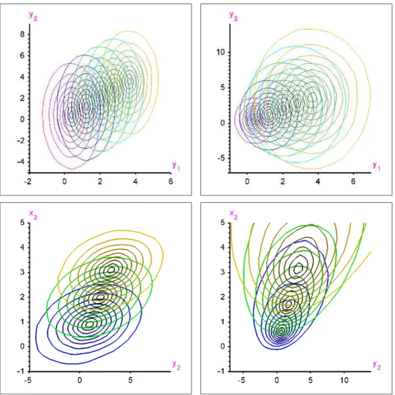
Finite-sample versions of all regression concepts above are obtained, simi-larly as in the location case (Section2), as the natural sample analogs of the corresponding population concepts; see Figures5 and 6 for an illustration. From a numerical point of view, Section5.2, with obvious minor changes, still describes how to compute the resulting regression quantile regionsR(regrn)(τ), withm and uy substituded fork and u, respectively.
The Kong and Mizera projection approach also readily generalize to the multiple-output regression setting. This issue is briefly addressed in Sec-tion 11.3 of [22]; see [28] for a detailed comparison with our approach. As for the conditional quantiles of Wei ([39]), their regression version shares the same local features as their location counterpart.
7. A real data application. In order to illustrate the implementabil-ity and data-analytical power of the concepts we are proposing, we now consider a real data example. Since a thorough case study is beyond the scope of this paper, we only present some very partial results of an investiga-tion of the body girth measurement dataset considered in [15]. That dataset consists of joint measurements of nine skeletal and twelve body girth di-mensions, along with weight, height, and age, in a group of 247 young men and 260 young women, all physically active. We refer to [15] for details; note, however, that thesen= 507 observations cannot be considered a ran-dom sample representative from any well-defined population, so that the
regression quantile contours we are providing below should be taken from a descriptive/illustrative point of view only.
For each gender, taking as regressors a constant term and (with nota-tion W) either weight, age, height, or the body mass index (defined as BMI:=weight/height2), we considered all 9+122
= 210 possible bivariate output regression models, and computed the regression tubes for τ = .01, .03, .10, .25, and.40, respectively. Three-dimensional pictures of those tubes are not easy to read, and we rather plot, for each of them, a series of five cuts. These cuts were obtained as the intersections of the regression tube under study with hyperplanes of the form w= w(p), where w(p) stands for the (empirical)pth quantile of the covariateW,p=.10 (black), .30 (blue), .50 (green), .70 (cyan) and .90 (yellow). The results are presented, for women,Y1 the calf maximal girth, andY2 the thigh maximal girth, withW the weight, age, BMI, and height, respectively, in Figure7.
Results look quite different depending on the choice of regressors. Re-gression with respect to weight shows a clear positive trend in location (all contours), along with an increasing dispersion, and an evolution of “principal directions”, yielding higher variability in calf than in thigh girth for lighter weights (horizontal first “principal direction”), while heavier weights tend to exhibit the opposite phenomenon (vertical first “principal direction”). Quite on the contrary, regression with respect to age apparently does not reveal any location trend: the inner contours almost coincide for all age cuts, and “principal directions” (roughly, parallel to the main bisectors) appar-ently do not change with age. However, the shapes of outer contours vary quite significantly with age, indicating an increasing (with age) simultaneous variability of both calf and thigh girth largest values. While the results for BMI look very similar to those for weight, a new phenomenon appears when height is the regressor, namely a clear regression effect for some contours (the inner ones) but not for the others, so that the asymmetry structure of the conditional distribution strongly depends on height: the conditional distributions seem much more asymmetric for low values of height than for the higher ones.
yield a much richer and subtle analysis of the impact of weight/age/BMI/ height on those body measurements than any traditional regression method can provide.
8. Final comments. This work presents a new concept of multivari-ate quantile based onL1 optimization ideas and clarifies the quantile nature of halfspace depth contours, while providing an extremely efficient way to compute the latter. The same concept readily allows for an extension of quantile regression to the multiple-output context, thus paving the way to a multiple-output generalization of the many tools and techniques that have been based on the standard (single-output) Koenker and Bassett concept of quantile regression. This final section quickly discusses several open prob-lems, of high practical relevance, that could now be considered.
First of all, Section 6 only very briefly indicates how our multivariate quantiles extend to the context of multiple-output regression; that exten-sion clearly calls for a more detailed study, covering standard asymptotic issues (limiting distributions, Bahadur representations) as well as robust-ness aspects (breakdown points and influence functions). Nonlinear quantile regression problems also should be addressed via, for instance, local linear methods.
The regression rank score perspectives (associated with linear program-ming duality) sketched in Section 5.1also look extremely promising, possi-bly leading to the development of a full body of multivariate, depth-related, methods of rank-based inference.
Finally, as mentioned in the Introduction and in Section3.1, various con-cepts introduced in this paper can be quite useful for inference. As an exam-ple, note that the symmetry (central, elliptical, or spherical) structure of P is reflected in the mappings
u7→λτuu/λ(τ∞) and u7→ kcτuku/c(τ∞),
with λ(τ∞) := supu∈Sk−1λτu and c(τ∞) := supu∈Sk−1kcτuk, as illustrated (with the corresponding empirical quantities, of course) in Figure8. A test of the hypothesis that the density ofZ is, e.g., spherically symmetric thus
could be based on (the empirical version T(n) :=T(Pn) of) a functional of the form T(P) := Z 1 0 Z Sk−1δ λ τu λ(τ∞) ,1 dσ(u)w(τ)dτ,
where δ(·,·) denotes some distance (such as that of Cram´er-von Mises), w some positive weight function over (0,1), and σ the uniform measure over Sk−1. Deriving the asymptotic properties of such statistics, however, clearly requires uniform versions of the asymptotic results in Theorem3.1
APPENDIX A
Proof of Theorem 3.1. The quantityηηηi,τττ(a,b) := J′uξξξi,τττ(a,b) is a sub-gradient for (a,b)7→ρτ(Ziu−b′Z⊥iu−a) since, for all (a,b′)′,(a0,b′0)′ ∈Rk, we have that ρτ(Ziu−b′Z⊥iu−a)−ρτ(Ziu−b′0Zi⊥u−a0)−(a−a0,b′−b′0)ηηηi,τττ(a0,b0) = (I[u′Zi−b′ 0ΓΓΓ′iuZi−a0<0]−I[u′Zi−b′ΓΓΓ′iuZi−a<0])(u ′Z i−b′ΓΓΓ′iuZi−a)≥0, irrespective of the value of Zi. Hence, interchanging differentiation and
expectation (which is justified in a standard way) shows that (a,b′)′ 7→
Ψτττ(a,b) (see Definition2.1) satisfies grad Ψτττ(a,b) = grad E[ρτ(Ziu−b′Z⊥iu−
a)] = E[ηηηi,τττ(a,b)]; see (3.2a)-(3.2b). Therefore,
grad Ψτττ(aτττ + ∆a,bτττ + ∆∆∆b)−grad Ψτττ(aτττ,bτττ)−Hτττ(∆a,∆∆∆′b)′ = Z Rk−1 Z (aτττ+∆a)+(bτττ+∆∆∆b)′x aτττ+bτ′ττx (f(zu+ ΓΓΓux)−f((aτττ +b′τττx)u+ ΓΓΓux)) (1,x′)′dz dx, and Assumption (A′n) yields that
kgrad Ψτττ(aτττ + ∆a,bτττ + ∆∆∆b)−grad Ψτττ(aτττ,bτττ)−Hτττ(∆a,∆∆∆′b)′k ≤C Z Rk−1 Z (aτττ+∆a)+(bτττ+∆∆∆b)′x aτττ+b′τττx |z−(aτττ +b′τττx)|sk(1,x′)′k (1 +k1 2(z+aτττ +b′τττx)u+ ΓΓΓuxk2)(3+r+s)/2 dz dx ≤C Z Rk−1|∆a+ ∆∆∆ ′ bx| |∆a+ ∆∆∆′bx|sk(1,x′)′k k(1,x′)′k3+r+s dx ≤Ck(∆a,∆∆∆′b)′k1+s Z Rk−1k(1,x ′)′k−(r+1)dx=o(k(∆ a,∆∆∆′b)′k),
as k(∆a,∆∆∆′b)′k → 0. This shows that (a,b′)′ 7→ Ψτττ(a,b) is twice
differ-entiable at (aτττ,b′τττ)′ with Hessian matrix Hτττ. Since, moreover,
Assump-tion (A′n) clearly ensures that E[kηηηi,τττ(a,b)k2] < ∞ for all (a,b′)′ ∈ Rk,
Theorem 4 of [27] applies, which establishes (3.16). Of course, (3.17) results from (3.16) by the multivariate CLT.
Recall that, under Assumption (A), the unique solution of (2.1) can be written as (aτττ,bτττ′)′ := (aτττ,(−ΓΓΓ′ucτττ)′)′, where (aτττ,c′τττ)′ denotes the unique
so-lution of (2.4). Similarly, any solution (aτττ(n),bτττ(n)′)′ of (2.5) is related to some
solution (aτττ(n),cτττ(n)′)′of (2.6) via the relation (a(τττn),bτττ(n)′)′= (aτττ(n),(−ΓΓΓ′uc (n)
τττ )′)′.
This allows for rewriting (3.16) as (A.1) √nPkJ′u aτττ(n)−aτττ cτττ(n)−cτττ ! =−√1 nH −1 τττ J′u n X i=1 ξξξci,τττ(aτττ,cτττ) +oP(1), as n → ∞. By first premultiplying both sides of (A.1) with PkJu, then using ΓΓΓuΓΓΓ′u = Ik−uu′ (which follows from the orthogonality of (u... ΓΓΓu)) andu′c(τττn)= 1 =u′cτττ, we obtain √ n a (n) τττ −aτττ cτττ(n)−cτττ ! =−√1 nPkJuH −1 τττ J′u n X i=1 ξξξci,τττ(aτττ,cτττ) +oP(1), asn→ ∞. LemmaA.1below therefore establishes (3.18). Again, the multi-variate CLT then trivially yields (3.19).
Finally, applying Theorem 6 in [27] (more precisely, applying the ver-sion (a) of Statement (3.8) in that theorem) withL =Ik and c= (aτττ,b′τττ)′
yields (A.2) nΨ(τττn)(aτττ,bτττ)−nΨτττ(n)(aτττ(n),bτττ(n))− 1 2n n X i,j=1 ξξξ′i,τττ(aτττ,bτττ)JuHτττ−1J′uξξξj,τττ(aτττ,bτττ) =oP(1), as n → ∞. Note that the third term is clearly OP(1) as n → ∞. The result then follows by dividing both sides of (A.2) by √n, and by using the identities λτττ(n) = Ψ(τττn)(aτττ(n),b(τττn)) (see the end of Section 5.1) andu′z−
b′τττΓΓΓ′uz−aτττ =cτττ′z−aτττ for allz∈Rk. Since (3.7) entailsλτττ = E[ρτ(c′τττZi−aτττ)],
the CLT yields (3.21).
In order to complete the proof of Theorem3.1, it is sufficient to establish the following lemma.
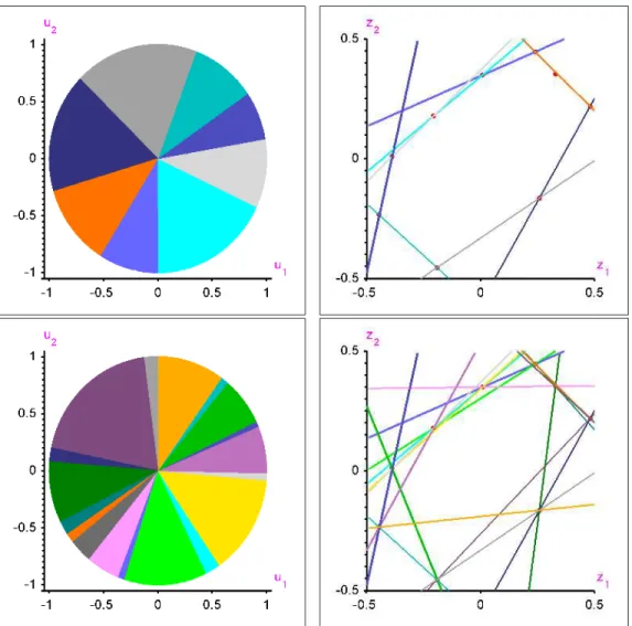
![Fig 1. The left plot contains n = 9 (red) points drawn from U ([ −.5, .5] 2 ), the centered bivariate uniform distribution over the unit square, and provides all τ -quantile hyperplanes for τ = .2](https://thumb-us.123doks.com/thumbv2/123dok_us/9975981.2490129/41.918.177.750.182.466/contains-centered-bivariate-uniform-distribution-provides-quantile-hyperplanes.webp)
![Fig 3. Tukey contours D (n) (τ ) (in green) obtained for n = 449 from U ([ −.5, .5] k ), N (0, 1) k , and t k1 (the products of k independent uniform, standard Gaussian, and Cauchy distributions, respectively), (a) for k = 2 and τ ∈ {.01, .05, .10, .15, .2](https://thumb-us.123doks.com/thumbv2/123dok_us/9975981.2490129/42.918.164.757.191.836/contours-obtained-products-independent-standard-gaussian-distributions-respectively.webp)

![Fig 7. Four empirical regression quantile plots from the body girth measurements dataset (women subsample; see [15])](https://thumb-us.123doks.com/thumbv2/123dok_us/9975981.2490129/46.918.176.744.227.778/empirical-regression-quantile-plots-girth-measurements-dataset-subsample.webp)

