Insurance Activities and Systemic Risk

(1)

ICIR Working Paper Series No. 19/15

Insurance Activities and Systemic Risk

Elia Berdin∗, Matteo Sottocornola†

This version: December 2015

Abstract

This paper investigates systemic risk in the insurance industry. We first analyze the systemic contribution of the insurance industry vis-`a-vis other industries by applying 3 measures, namely the linear Granger causality test, conditional value at risk and marginal expected shortfall, on 3 groups, namely banks, insurers and non-financial companies listed in Europe over the last 14 years. We then analyze the determinants of the systemic risk contribution within the insurance industry by using balance sheet level data in a broader sample. Our evidence suggests thati)the insurance industry shows a persistent systemic relevance over time and plays a subordinate role in causing systemic risk compared to banks, and that ii) within the industry, those insurers which engage more in non-insurance-related activities tend to pose more systemic risk. In addition, we are among the first to provide empirical evidence on the role of diversification as potential determinant of systemic risk in the in-surance industry. Finally, we confirm that size is also a significant driver of systemic risk, whereas price-to-book ratio and leverage display counterintuitive results.

Keywords: Systemic Risk, Insurance Activities, Systemically Important Financial Institutions

JEL Classification: G01, G22, G28, G32

The content of this study does not reflect the official opinion of EIOPA. Responsibility for the information and views expressed therein lies entirely with the authors.

∗

Affiliation: International Center for Insurance Regulation and Center of Excellence SAFE Sustainable Ar-chitecture for Finance in Europe, Theodor W. Adorno Platz 3, Goethe University Frankfurt, D-60629 Frankfurt am Main., Germany. Contact: telephone +49 6979833876, e-mailberdin@finance.uni-frankfurt.de.

†

Affiliation: EIOPA, Westhafenplatz 1, D-60327 Frankfurt am Main., Germany. and Center of Excel-lence SAFE Sustainable Architecture for Finance in Europe, Theodor W. Adorno Platz 3, Goethe Univer-sity Frankfurt, D-60629 Frankfurt am Main., Germany. Contact: telephone +49 69951119416, e-mail

mat-teo.sottocornola@eiopa.europa.eu.

‡

The authors are grateful to Christian Brownlees, J. David Cummins, Giulio Girardi, Helmut Gr¨undl, Felix Irresberger, Anne Kleffner, Loriana Pelizzon, Gregor N.F. Weiß, Mary A. Weiss and to the participants at the following conferences and seminars for advice and suggestions: the 2015 Annual Meeting of the German Insurance Association (Berlin), Finance Brown Bag Seminar at Goethe University (Frankfurt), the Systemic Risk Work-shop 2015 at Temple University (Philadelphia), the European Systemic Risk Board Seminar on Insurance 2015 (Frankfurt) and the World Risk and Insurance Economics Congress 2015 (Munich). We gratefully acknowledge research support from the Research Center SAFE, funded by the State of Hesse, initiative for research LOEWE.

(2)

1 Introduction

Following the 2007-2009 financial crisis and the 2010-2012 European sovereign debt crisis, the concept of systemic risk has become increasingly relevant.1 After the collapse of Lehman Brothers in particular, the debate on systemic risk has been primarily focused on banks.2 However, recent empirical evidence suggests that institutions not traditionally associated with systemic risk, such as insurance companies, also play a prominent role in posing systemic risk. In particular, some authors find that the insurance industry has become a non-negligible source of systemic risk (e.g. Billio et al. (2012) and Weiß and M¨uhlnickel (2014)). This is partially in contrast to other authors, who do not find evidence of systemic relevance for the industry as a whole (e.g. Harrington (2009), Bell and Keller (2009) and Geneva Association (2010)). Finally, other authors take a more granular perspective and argue that insurance companies might be systemically relevant, but that such risk stems from non-traditional (banking-related) activities (Baluch et al.(2011) andCummins and Weiss(2014)) and that in general, the systemic relevance of the insurance industry as a whole is still subordinated with respect to the banking industry (Chen et al.,2014).

As the current literature does not provide a common understanding and clear evidence regarding the systemic relevance of the insurance industry and the activities connected thereto, we thus aim with this paper to fill this gap. In particular, we investigate i) the systemic relevance of the insurance industry vis-`a-vis other industries andii) the key drivers of systemic risk within the insurance industry.

To do so, we test 3 equity return-based measures of systemic risk, namely 1) the indexes based on linear Granger causality tests proposed byBillio et al. (2012) (Granger test), 2) the conditional value at risk proposed by Adrian and Brunnermeier(2011) (∆CoVaR) and 3) the dynamic marginal expected shortfall proposed by Brownlees and Engle (2012) (DMES), on 3 groups, namely banks, insurers and non-financial companies, all listed in Europe. We test the systemic relevance of each institution with respect to its own industry (intra-industry), with respect toother industries and with respect to thetotal system. Based on these estimations, we rank financial institutions according to their average systemic risk contribution over time and create anindustry composition index. Finally, we investigate the drivers of systemic risk within

1_{Throughout this paper, we rely on the definition of systemic risk given by the Group of Ten (2001):} _Systemic

risk is the risk that an event will trigger a loss of economic value or confidence in a substantial segment of the financial system that is serious enough to have significant adverse effects on the real economy with high probability.

2

(3)

the insurance industry by focusing on the asset and liability composition of insurers’ balance sheets.

Our evidence suggests that the insurance industry tends to persistently pose systemic risk over time and to play a subordinate role with respect to the banking industry, with some distinction in specific periods when the insurance industry becomes more systemic than the banking industry. Furthermore, we show that insurers with a relatively larger proportion of non-insurance-related activities tend to pose more systemic risk. In addition, we are among the first to provide evidence on the role of diversification of the asset portfolio with respect to systemic risk. We also find and confirm previous evidence that price-to-book and size do matter, whereas leverage seems to play an ambiguous role. Finally, our results are robust across different specifications and different samples.

The paper is organized as follows: section 2 provides a comprehensive literature review, section 3describes the methodology and the data; section4 describes the results and section5

concludes the analysis.

2 Literature review

The literature on systemic risk has been steadily growing following the crises.3 In particular, a wide range of new empirical methods for testing the systemic risk contribution of financial institutions has been proposed. Moreover, both academia and regulators have dedicated more attention to the role of non-banking financial institutions: among these institutions, insurance companies emerged as a potential source of systemic risk.4

Before the crises, there was substantial agreement among scholars in considering the in-surance industry to be not systemically relevant. However, in the literature that emerged in the aftermath of the crises, although many studies still consider the insurance industry non-systemically relevant as a whole, some authors argued that the insurance industry might have become systemically relevant, particularly in a number of specific activities. Many agree in ranking core life insurance activities as the most systemically relevant, whereas core non-life insurance activities are considered the least systemically relevant. In addition, an ambiguous position is attributed to reinsurance activities.5

3_{By crises we mean both the 2007-2009 financial crisis and the 2010-2012 European sovereign crisis.} 4

A comprehensive review of the literature on systemic risk in the insurance industry is provided byEling and Pankoke(2012).

5

(4)

Cummins and Weiss (2014) argue that according to primary indicators and contributing factors, such as leverage, interconnectedness and size of exposure to credit, market and liquidity risk, the most systemically relevant activities are non-core activities conducted mainly by life insurers. Moreover, Harrington(2009) concludes that systemic risk is potentially higher for life insurers due to the higher leverage, sensitivity to asset value decline and potential policyholder withdrawals during a financial crisis, whereas systemic relevance is relatively low in property and casualty (P&C) insurance due to low leverage ratios. Furthermore, by analyzing the takeover of AIG by the Federal Government in the United States, the author suggests that the AIG crisis was heavily influenced by the credit default swaps (CDS) written by AIG financial products and not by more traditional insurance products written by AIG’s regulated insurance subsidiaries. TheGeneva Association(2010) conducted an analysis on the role played by insurers during the 2008 crisis and argues that the substantial differences between banks and insurance companies, namely the long-term liability structure of insurers compared to banks and the strong cash flow granted by the inversion of the cycle, is sufficient to rule out systemically any implications of the insurance industry during the financial crises aside from the companies highly exposed towards non-core insurance activities. Bell and Keller(2009) analyze the relevant risk factors stemming from an insurance company and conclude that traditional insurers do not pose systemic risk and, as a consequence, are neither too big nor too interconnected to fail, and that insurers engaging in non-traditional activities, such as CDS, can pose substantial systemic risk. Baluch et al.(2011) provide further arguments for the lower relevance of P&C activities and the higher relevance of non-traditional life activities: the authors argue that the fundamental reason lies in the bank-like business type and the massive amount of interconnectedness needed to run these kinds of activities.

The concept of interconnection, as expressed, among others, in Baluch et al. (2011), rep-resents the link between analyses focused on industry-specific characteristics and more general equity-based analyses in which prices reflect all the necessary information.6 Equity-based mea-sures aim to measure the effect of one institution on the system or vice versa and the level of interconnectedness of the system. These measures include the ∆CoVaR (Adrian and Brunner-meier(2011)), the MES and DMES (Acharya et al.(2010) andBrownlees and Engle(2012)), the Distressed Insurance Premium (DIP) (Huang et al.(2012)), Contingent Claims Analysis (CCA)

the reinsurance business. On the other hand,Cummins and Weiss(2014) claim that, despite historical evidence, both life and P&C insurers are exposed to reinsurance crises.

6

(5)

(Gray and Jobst(2011)) and the linear and non-linear Granger causality test proposed byBillio et al. (2012). According to such measures, the insurance industry displays different degrees of systemic relevance. For instance, Acharya et al. (2010) argue that insurance companies are overall the least systemically relevant financial institutions. The authors provide estimations of the spillover effects through a measure of conditional capital shortfall, i.e. Systemic Expected Shortfall (SES) and MES for the U.S. financial industry during the 2007-2009 crisis. The con-tribution of Adrian and Brunnermeier (2011) extends the traditional value at risk concept to the entire financial system conditional on institutions being in distress. The authors apply the measure to a set of institutions, including banks and thrifts, investment banks, government sponsored enterprises and insurance companies, finding no distinction among the systemic rel-evance of different types of institutions. In contrast, Billio et al. (2012) apply the linear and non linear Granger causality test to a sample of banks, insurers, hedge funds and broker dealers operating in the U.S. in order to establish pairwise Granger causality among equity returns of financial institutions. Their evidence suggests that during the 2008 financial crisis, besides banks, insurance companies were a major source of systemic risk. This conclusion is partially in contrast to Chen et al. (2014): the authors agree that the linear Granger causality test attributes a systemic relevance to insurance companies comparable to the systemic relevance of banks. However, they argue that when applying a linear and non-linear Granger causality test to the same series corrected for heteroskedasticity, banks tend to cause more systemic risk and for longer periods of time then insurance companies. Weiß and M¨uhlnickel (2014) and

Bierth et al.(2015) focus directly on the link between equity-based systemic risk measures and industry-specific fundamentals. Weiß and M¨uhlnickel (2014) estimate the systemic risk contri-bution based on ∆CoVaR and MES for a sample of U.S. insurers during the 2007-2008 crisis, inferring that insurers that were most exposed to systemic risk were on average larger, relied more heavily on non-policyholder liabilities and had higher ratios of investment income to net revenues. Bierth et al. (2015) analyze a much broader sample of insurers over a longer time horizon and find that the systemic risk contribution of the insurance sector is relatively small. However, they also argue that the contribution of insurers to systemic risk peaked during the 2007-2008 financial crisis and find that the interconnectedness of large insurers with the insur-ance industry is a significant driver of the insurers exposure to systemic risk. Finally, they argue that the contribution of insurers to systemic risk appears to be primarily driven by leverage, loss ratios and funding fragility.

(6)

Concluding, the existing literature provides a diversified and controversial picture of the systemic relevance of the insurance industry. In particular, there is a lack of empirical evidence on the link between industry-specific activities and their contribution to systemic risk measured by equity prices. On the one hand, some studies argue that due to its nature, the insurance industry does not pose systemic risk, and therefore measures based on equity values might be misled by spurious effects (e.g. increased risk aversion vis-`a-vis the financial industry); on the other hand, some studies provide evidence on the role of the insurance industry in posing systemic risk and its growing importance in recent years. Yet, few studies attempt to analyze empirically the relative position of the insurance industry vis-`a-vis other industries and the key drivers within the insurance industry. This contribution thus aims at bridging this gap by investigating the systemic risk contribution of the insurance industry relative to other industries and the key determinants on the balance sheet of insurers. Moreover, this is the first study that focuses on European insurers.

3 Methodology & Data

Our analysis consists of 2 steps:

i) we conduct an analysis of the systemic risk contribution of the insurance industry vis-`a-vis other industries using equity-based measures of system risk (industry analysis);

ii) we then conduct an empirical analysis at balance sheet level of a broader sample of Euro-pean insurers based on their systemic risk contribution (analysis of fundamentals).

3.1 Systemic Risk Measures and Rankings of Systemic Risk Contributions

For the industry analysis, we apply 3 widely used equity-based measures of systemic risk: 1)the Granger causality testproposed byBillio et al.(2012), 2)the ∆CoVaRproposed by

Adrian and Brunnermeier(2011) and3)theDMESproposed byBrownlees and Engle(2012).7 We identify 3 groups, namely banks, insurers and non-financials. In addition, for each systemic risk measure and for each group, we distinguish between 3 cases: the average contribution of the individual institution belonging to a single group a) within its group (intra-industry), b) towards the other 2 groups (other industries) and c) towards all 3 groups (total system).8 We

7

An extensive mathematical treatment of the 3 measures is provided in AppendixA.1.

8

(7)

then calculate the average contribution of each industry by taking the median of the month (for the ∆CoVaR and the DMES, whereas the Granger causality test is calculated on a monthly basis) and the average through the institutions of the same industry. Finally, at each point in time, we rank the institutions of the total system from the most to the least systemically relevant according to each systemic risk measure. We then select the top 10 institutions at each point in time and calculate the relative weight of each industry within the top 10 over time, thereby creating an index. More formally, the group of selected institutions at each point in time is defined as

S_tk={i1,t > ... > in,t> ... > i10,t} (1)

in whichinrepresents an institution ranked from the most to the least systemic (withn= 1→

most systemic) according to the k measure, with k = Granger, ∆CoVaR, DMES. Then, the index for each systemic risk measurek is obtained as follows

I_tk =                P10 n=11in,t=Bank 10 P10 n=11in,t=Insurer 10 P10 n=11in,t=N on−F inancial 10 (2)

in which1is an indicator function that takes value 1 if the condition (e.g. ifin=Bank) is met

and 0 otherwise. Sums are then scaled between 0 and 1. Finally, we group all 3 indexes and form the total index, which is given by

I_ttot =                P k P10 n=11in,k,t=Bank 3·10 P k P10 n=11in,k,t=Insurer 3·10 P k P10 n=11in,k,t=N on−F inancial 3·10 (3)

It is worth remarking that the 3 systemic risk measures that we test in the analysis tend to represent different phenomena and therefore need to be correctly interpreted. The Granger causality test is a measure that allows us to quantify the degree of connectedness of an insti-tution vis-`a-vis a system of institutions. By creating a network of pairwise statistical relations, we can observe not only the degree of interdependence, but also the direction thereof. The measure is thus a good proxy for an analysis at an aggregate level (for example industry or other clusters), but its estimation could become cumbersome when the objective is to test the

(8)

individual interconnection with respect to a system of institutions as proxy for the market.9 The ∆CoVaR measures the difference between the CoVaR conditional on the distress of an institution, i.e. the value-at-risk of the system conditional on an institution being in distress and the CoVaR conditional on the normal state of the institution. It is therefore able to capture the marginal contribution of a particular institution to the overall systemic risk. One of the main advantages of such a measure is its ability to capture the individual contribution of each institution to the system. Finally, the DMES measures, in a dynamic setting, the expected drop in equity value of an institution when the system is in distress. It is worth mentioning that this is not a direct measure of systemic risk, but is highly related to it. The contribution of

Brownlees and Engle(2012) originates from the proposal ofAcharya et al.(2010), in which the marginal expected shortfall of an institution coupled with its leverage, originate the systemic expected shortfall (SES), i.e. the expected capital shortage of an individual firm conditional on a substantial reduction in the capitalization of the system. The authors propose a similar measure called SRISK, which is based on a dynamic estimation of the MES and leverage ratios. A major advantage of such a contribution is its ability to capture time-varying effects, effects which are not observable following Acharya et al. (2010). However, bothBrownlees and Engle

(2012) and Acharya et al. (2010) estimate such systemic risk measures relying on the estima-tion of the marginal expected shortfall (MES) and of pre-determined leverage ratios: in order to avoid additional assumptions that might cast doubts on the reliability of the estimation,10 we simply rely on the directly observable part of the measure, i.e. the DMES, which is sufficient to provide information on the individual fragility of the individual institution with respect to market tail events, which in turn have potential systemic implications.11

3.1.1 Data

The data set for the industry analysis consists of equity returns of 60 companies listed in Europe over a time window of 14 years, from January 1999 to December 2013, which becomes 17 years (i.e. from January 1996 to December 2013) for the Granger causality test due to the

9

By market, we essentially mean a broad measure and proxy for the (real) economic activity such as a major stock index. Throughout the paper, we therefore interchangeably use the terms system and market as (almost) perfect substitutes.

10_{However, it is worth noting that}_{Brownlees and Engle}₍₂₀₁₂_{) provide a series of robustness checks on the}

stability of the parametrization of the SRISK measure.

11

Another major issue we face regarding the estimation of the SRISK is the frequency of the accounting data: since we focus on European insurers, we do not possess sufficiently long quarterly series of balance sheet data.

(9)

lag on the series.12 For each group, we select the top 20 institutions in terms of capitalization from STOXXr Euro 600 Banks, STOXXr Euro 600 Insurance and STOXXr Europe 600 for banks, insurers and non-financials respectively.13 Table 1 reports the list of the selected institutions, while table 2 reports the industry distribution of non-financial institutions. Data were collected both at daily and monthly frequencies. Table 3 reports the summary statistics of the 3 groups. To calculate the ∆CoVaR, we rely on a set of state variables as proposed in

Adrian and Brunnermeier (2011), namely i) Market volatility (VIX for Europe), ii) Liquidity spread (3M Repo - 3M Bubill), iii) change in the short-term interest rate (3M Bubill), iv) the slope of the yield curve (10Y Bund - 3M Bubill), v) credit spread (BAA 5-7Y Corporate (Bank of America) - EURO Sovereign 5-7Y (Barclays)), vi) market returns (STOXX EURO 600 All shares). Table 4 reports the summary statistics for the state variables. Finally, tables

5, 6 and 7 report the summary statistics of monthly and daily returns for banks, insurers and non-financials respectively.

3.2 Systemic Risk Measures and Insurers’ Fundamentals

For the analysis of fundamentals, we investigate the relation between asset and liability compositions and systemic risk measures. In particular, we focus on items on the balance sheet rather than on the income statement, i.e. measures of stock rather than flow. This is justified by the fact that the insurance industry is a liability-driven business which often entails a long-term horizon in which the ability to maintain outstanding financial promises might change over time.14 The outstanding stocks, and therefore the underlying past and current capital allocation decisions, i.e. underwriting decisions and consequent asset allocation, thus have a profound impact on the dynamics of the value of the institution, especially when sudden changes in market conditions, such as the 2007-2009 financial crisis, occur.15 Thus, it is worth dissecting the different components of the insurance balance sheet in order to understand where potential sources of systemic risk are. In addition, the analysis focuses on the business conducted at

12

Data were downloaded from Datastreamr.

13_{Within each group, companies are ranked according to the yearly average market capitalization over the}

14-year time frame. We selected those companies which were continuously listed over the period.

14_{This is particularly true in the life and health business segment.} 15

In a public speech, the President of the European Central Bank (ECB) Mario Draghi emphasized this point and stated that ”(...) The models were built on flows, with little or no attention paid to stocks. But it was precisely from stocks that the irregularities and hence the crisis arose. Non linearities arise on a balance sheet

when capital falls to zero and the agent goes into default (...)“ (Draghi,2012). For a much broader perspective

(10)

shareholders’ risk, namely excluding items for which risk is borne by policyholders.16 In this part of the analysis, we are thus able to test which features drive the contribution of insurers to systemic risk.

In order to test the relation between relevant balance sheet items and systemic relevance, we run OLS regressions with yearly fixed effects of the lagged individual insurer balance sheet characteristics on the individual systemic risk measure.17 We specify a model that includes both asset and liability based indicators. This model allows on the one hand to separately analyze the systemic implications stemming from underwriting and investment decision18 and on the other hand to avoid potential biases, such as omitted variables.

The baseline model for the ith insurer is given by the following:

SRi_t=β0+β1·P rice−to−bookit−1+β2·Leveragei,A/Lt−1 +β3·Sizei,A/Lt−1 +

X

j

βj·Xj,ti −1+it (4)

in which Price-to-book is the market value to book value ratio, LeverageA is the ratio between tangible assets and tangible equity and LeverageL the ratio between liabilities and tangible equity, SizeA is the logarithm of tangible assets and SizeL is the logarithm of liabilities.19 We specify both Leverage and Size in 2 different (but analogous) ways in order to avoid multicollinearity problems when regressing on the relevant balance sheet items and proxies.

Xj includes a set of balance sheet items and proxies for specific factors which may influence

the systemic risk contribution of an insurance company. These include Concentration, Invest-ment Quality,Fixed Income Assets,Equity Assets, Cash,Insurance Activities,Total Debt and Separate Accounts. More specifically, Concentration is the Herfindahl-Hirschman index (H-H) with respect to asset classes of the portfolio’s holdings which broadly captures the degree of diversification of the portfolio20; Investment Quality is the amount of at least A-rated assets which proxies the quality of the asset allocation with respect to credit risk21 andFixed Income Assets,Equity Assets and Cash are the amount of fixed income, equity and cash assets classes

16

This business is usually categorized as unit-linked or separate account business.

17_{We introduce the lag as to avoid endogeneity issues.} 18

It is worth noticing how underwriting decisions tend to shape investment decisions consistently with the typical liability-driven business approach of the insurance industry, but decisions on the asset allocation might be also influenced by other factors, such as the need to deliver investment performances, and not being limited to the replication of the liability portfolio.

19_{Price-to-book}_,_Leverage_and_Size_{are usually identified as key drivers of systemic risk in financial institutions,}

see for instanceWeiß and M¨uhlnickel(2014).

20

The H-H index is a widely applied measure of concentration: it is computed as follows

P

ix2i

(P

ixi)2. For its original applications, seeHirschman(1964).

21

(11)

respectively. Finally, Insurance Activities is the amount of insurance activities among total activities,Total Debt is the amount of debt which includes senior debt, i.e. mainly deposits for banking activities, and subordinated debt, Separate Accounts is the amount of business which is not at shareholder risk.22

3.2.1 Hypotheses and Expected Contributions

It is worth clarifying beforehand the expectations with respect to the marginal contribution of single factors on systemic risk. To this purpose, we formulate 2 ex-ante hypotheses: the first one is the following

H.1) The Systemic Risk contribution of insurers is mainly driven by the liability side, i.e. its capital structure.

In particular, we expect Insurance Activities as a proxy for traditional insurance business, to exert a negative contribution to systemic risk, i.e. _{∂ I.A.}∂SR <0; by contrastTotal Debt is expected to positively contribute to systemic risk, i.e. _{∂ T .D.}∂SR > 0: this could be loosely interpreted as proxy for banking activities, since deposits are classified as senior debt, but also more broadly as non-insurance activities. Finally, Separate Accounts (or unit-linked business) is expected to be insignificant as most of the risk connected to such business are transferred to policyholders. An implication of such hypothesis is that the asset side tends to play a subordinated role in posing systemic risk in insurance, although its level of diversification and its credit quality might turn out to be relevant factors since underwriting decisions tend to be replicated in the asset side.23 More formally, Concentration is a proxy for the degree of diversification of the asset portfolio. By a micro perspective, a higher degree of diversification could have a positive impact on the single institution in terms of risk diversification. However, by a macro perspective a higher degree of diversification could have a negative impact on the overall system due to the higher degree of interconnectedness among institutions. 24 Hence, as interconnectedness is a potential source of systemic risk (Billio et al.,2012), we formulate a second hypothesis:

H.2) A higher diversification of investments is associated with a higher contribution to systemic risk.

22

Table8reports a detailed overview of the variables used throughout the analyses.

23_{In other words, (re)insurers focused on traditional insurance activities adopt asset and liability management}

strategies through which risks undertaken on the liability side are hedged (replicated) through the asset side.

24

An extensive treatment of the argument is provided among others byDas and Uppal(2004),Wagner(2010),

(12)

More specifically we expectConcentrationto negatively contribute to the systemic relevance of an institution, i.e. ∂SR_{∂ C.} <0. In addition, also Fixed Income Assets,Equity Assets and Cash might be significant contributors to systemic risk, in particular bonds might be expected to display a negative sign due to the generally lower degree of risk compared to equity, which in turn we expect to be a positive contributor and cash can be expected to display a negative sign as it could be loosely interpreted as a proxy for liquidity.

Finally, Price-to-book,LeverageA/L_and _SizeA/L_{are in general positive contributor to}

sys-temic risk in financial institutions, although in the insurance context it might not always be the case.25

3.2.2 Data

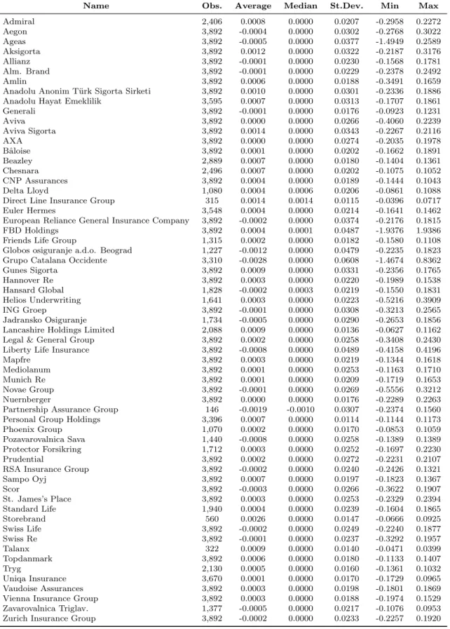
For the analysis of fundamentals, we rely on a larger data set of insurers listed in Europe. We were able to collect both market data and balance sheet data for 61 European insurers from SNL Financials. Tables 9 and 10 report summary statistics for equity returns of the insurers and balance sheet variables. Table11 displays the correlation matrix of balance sheet variables. Data for balance sheet variables is available from 2005 onwards, therefore the analysis of fundamentals can only cover the period between 2005 and 2013.

To test the relation between balance sheet composition and systemic risk contributions, we rely on 2 of the 3 measures that we estimated in the industry analysis, namely the ∆CoVaR and the DMES. This is due to the fact that while we can estimate these 2 measures using a representative index, this is no longer possible for the Granger causality test. In fact, for the purpose of the analysis, it is convenient to measure the marginal effect of each institution vis-` a-vis the system, which can be proxied through a broad equity index.26 Due to data availability, we use the FTSE All shares as proxy for the system.27 For the analysis of fundamentals, we thus focus on the ∆CoVaR and the DMES. To match the yearly frequency of the balance sheet data, we estimate daily ∆CoVaR and DMES, then take the median of the month and average through the year.28

25_{See for instance}_{Bierth et al.}₍₂₀₁₅_). 26

A similar approach is proposed inBierth et al.(2015) andBrunnermeier et al.(2012).

27_{For the sake of consistency, we would have employed the Euro STOXX total market, but unfortunately the}

total return index is only available from 2002 onwards. Therefore, we use the FTSE All shares as a substitute and proxy for the European market as a whole.

28

The systemic risk measures were re-estimated using the FTSE All shares as a system: not all of the 61 insurers were continuously listed between January 1999 and December 2013, therefore we calculated the measures with the available time series.

(13)

4 Empirical Results

4.1 Systemic Risk Measures and Rankings of Systemic Risk Contributions

4.1.1 The Granger causality test (Billio et al., 2012)

Figure 1 reports the evolution over time of the total number of causing (Granger-causal) significant connections over the total number of possible connections from a single institution belonging to each group towards its own industry (intra-industry). During the pre-crisis period, a generalized decrease in the connectivity level can be observed across the 3 groups: particularly in the period from 1999 to the end of 2004, the level of connectivity goes from roughly 20-25% to 10-15%; starting from 2005 onwards, the level of intra-industry connectivity among banks and insurers increases rapidly, spiking at 35-40% around the time of Lehman filing for bankruptcy and the subsequent AIG bailout. For non-financials, although the index signals an increase of the connectivity level, a Lehamn effect is much less visible. The filing for bankruptcy and the subsequent AIG bailout thus represent more of a shock to the financial industry than to the non-financial industry. The aftermath of Lehman in fact signals a clear increase in the connectivity level among banks: non-financials continue to display relatively lower levels of connectivity, whereas insurers tend to span halfway between banks and non-financials.

Figure 2 reports the evolution over time of the total number of Granger-causal significant connections over the total number of possible connections from each group towardsother indus-tries. The upper graph displays the average number of receiving (Granger-causal) connections for a single institution in each group from other industries. We can observe a clear pre- and post-Lehman trend which is consistent with the shock to the financial system as recorded in figure 1: before the filing for bankruptcy of Lehman, financial institutions tended to act as receivers more than non-financials; after Lehman the opposite occurs, with non-financials being net receivers. The lower graph displays the number of causing (Granger-causal) connections for each group from other industries. Clearly, the trend now follows opposite directions, with financial institutions becoming the net causer after Lehamn: in particular, banks from 2006 up to Lehman play a much stronger role compared to insurers, and the same tendency can be observed from 2009 to 2012. Once again, we can observe a subordinated role of insurers compared to banks as a cause of systemic risk, with a consequent role of net receiver played by non-financials.

(14)

(Granger-causal) significant connections over the total number of possible connections from each group towards the total system. Once again, insurers tend to be subordinated compared to banks in causing as well as receiving systemic risk: even though a unique trend over time does not emerge, we can still observe how from 2007 through to 2013, insurers persistently pose less systemic risk compared to banks, with an increase in this difference from 2009 onwards.

In summary, the outcome provided by the Granger causality test provides a fairly clear picture over time of receivers and causers of systemic risk: non-financials behave as causers during tranquil periods and as net receivers during crises, whereas banks appear to be the most prominent causers of systemic risk in the aftermath of a crisis. In particular, among financial institutions, insurers display a more ambiguous behavior compared to banks and on average play a subordinated role compared to banks, especially during the 2007-2009 financial crisis and its aftermath. This is in line with existing findings for American insurance companies.29

4.1.2 ∆CoVaR (Adrian and Brunnermeier, 2011)

Figure 4 reports estimations of the average individual institutions’ ∆CoVaR within its in-dustry (intra-industry). The figure displays a strong differentiation between financial and non-financial institutions. Banks and insurers present the lowest values, with the 2 curves almost perfectly co-moving over the whole time window. Nevertheless, differences between banks and insurers do exist, especially in the aftermath of the crisis, where banks persistently tend to register lower values compared to insurers, with differences of up to 1 percentage point around the European sovereign crisis, i.e. between 2011 and 2012. Furthermore, a striking difference emerges when comparing non-financials with banks and insurers: with the Granger causality test, non-financials are consistently less interconnected within themselves and display persis-tently much higher values.30

Figure5reports results for the average individual institutions’ ∆CoVaR towardsother indus-tries: pre-crises periods are clearly dominated by non-financials, whereas during and after the Lehman bankruptcy, banks and insurers become systemically more relevant, with non-financial companies still displaying a relatively higher contribution to systemic risk. It is clear that by changing the composition of the reference system towards which we estimate the measure, effects differ quite substantially: by considering the marginal effects of an institution towards other

29

See, among others,Chen et al.(2014).

30

Please note that we consider lower values to be a sign of higher systemic relevance, since the measure estimates market value losses.

(15)

industries, we can observe the spillover effects that one industry has onto other industries, and not surprisingly, non-financials had a higher influence on banks and insurers before the financial crisis occurred. This is mainly due to the exposure of the financial sector towards all other sectors rather than vice-versa.31 This once again provides evidence on the financial nature of the crisis.

Finally, figure6 reports the results of the average individual institutions’ ∆CoVaR towards thetotal system. Here, it is worth noting that before the bankruptcy of Lehman, financials and non-financials display small differences in values, whereas after the crisis, the contribution to systemic risk of financial institutions increases dramatically, with banks once more dominating insurers in terms of marginal contribution. Even though the differences appear modest, we should stress the fact that the measure is estimated on daily returns and averaged through many institutions, therefore the average marginal contribution of banks after 2008 can be estimated as being roughly 20% higher compared to insurers, which makes it considerably higher.

In summary, ∆CoVaR provides a fairly clear indication of the behavior of financial and non-financial institutions, which is in line with the Granger causality test. Furthermore, if we consider the estimations of thetotal system to be more representative of the role of each group in posing systemic risk, insurers again tend to play a subordinated role compared to banks.

4.1.3 DMES (Brownlees and Engle, 2012)

Figure7reports the results for the average marginal contribution of the individual institution within its industry (intra-industry). The pattern of each group is comparable with the one obtained with the other 2 measures, and in particular with the ∆CoVaR. The 2 measures present the same peaks during the financial crises and report a higher level of systemic riskiness after the crises compared to the pre-crises period. Differences from the previous measures can be found in the spikes at the end of 2001 and 2003 reported by DMES: these spikes are mainly driven by the insurance industry and can be traced back to industry-specific events such as 9/11 and severe natural catastrophes occurring in Europe in 2003. Consistent with the design of the measure, these peaks are well captured by DMES due to its focus on tails of the distributions, i.e. severe events. In general, financial institutions report lower average DMES values than non-financial institutions, with some differences between banks and insurers depending on the period: in the aftermath of the crises, banks pose more risk than insurers.

31

(16)

Figure 8 reports results for the average marginal contribution of the individual institution towards other industries: on the one hand, the measure indicates once more the distinction between financial and non-financial institutions, with the latter being overall less exposed to the financial sector; on the other hand, banks and insurers appear to be substantially equal in terms of contribution, with banks dominating in the aftermath of Lehman.

Finally, figure 9 reports the results for the average marginal contribution of the individual institution towards thetotal system. There is no significant difference from the results presented in both the Granger causality test and in the ∆CoVaR, which in turn confirms our results.

In summary, DMES confirms the outcome of the 2 other measures, attributing the higher systemic relevance to financial institutions, among which insurers prevail before Lehman and banks in its aftermath.

4.1.4 Systemically Important Financial Institutions (SIFIs)

We also report the average results towards thetotal systemfor those insurers labeled as SIFIs: this distinction is particularly relevant, since regulators indicated some common characteristics among these institutions which should make them more systemically relevant compared to the median insurer. It is thus worth analyzing their individual behavior vis-`a-vis the total system. Figure10 shows a higher average degree of causality compared to the full insurance group with significant peaks which can be observed during the Lehman bankruptcy. In general, we can observe that despite a higher causality compared to non-SIFIs, this sub-group of institutions still tends to play a minor role compared to banks in the aftermath of the Lehman crisis. Figure 11 reports a widespread increase of systemic contribution of SIFI insurers measured by ∆CoVaR in comparison to the full insurance sample and even compared to banks. The contribution towards thetotal system is the highest among the 3 groups throughout the period. Finally, figure12reports the result for the DMES: among the 3 measures, the DMES displays the smallest differences between SIFI insurers and non-SIFI insurers, with the period following the Lehman bankruptcy recording the systemic contribution of SIFIs as being significantly inferior to the contribution of banks.

4.1.5 Rankings

In order to provide a straightforward representation of the systemic relevance of the 3 groups according to the 3 measures, we display in figure13the 10 most systemically relevant institutions

(17)

grouped by industry at each point in time. The Granger causality test and the ∆CoVaR alternatively rank banks during crises and non-financials during tranquil periods as the most systemically relevant companies with a key distinction: banks are always present throughout the period, whereas non-financials disappear after the Lehman crisis. Insurers, despite always being present in the top 10 sub-group throughout the period, still play a subordinated role compared to banks. The DMES attributes a predominant role to insurance companies before the Lehman bankruptcy and to banks afterwards. The measure associates to non-financials an ancillary role only in tranquil periods. The systemic relevance of the 3 groups is finally summarized into a synthetic indicator that displays at each point in time the industry composition of the top 10 most systemic institutions according to the 3 measures.32 The index clearly shows that non-financials dominate the index before Lehman, whereas banks dominate it thereafter. In contrast, insurers always tend to play a subordinated role both before and after the Legman bankruptcy.

In conclusion, we can summarize our findings as follows: i) the 3 measures make a clear distinction between financial and non-financial institutions; ii) among financial institutions, banks dominate insurers in terms of contribution to systemic risk in the aftermath of the financial crises, with insurers nevertheless displaying a persistent contribution to systemic risk over time; iii) there is no clear-cut evidence on higher systemic relevance of SIFI insurers; iv) trends in systemic risk contributions are time-dependent and tend to change rapidly, making the choice of the time span of analysis a crucial variable. Moreover, it is worth mentioning that the 3 measures were developed to capture different features of the systemic risk contribution of institutions, therefore inconsistencies over time should not be seen as lack of accuracy, but rather as emphasis on different factors that contribute to systemic risk.

In the next section, we analyze the determinants behind the systemic contribution of insur-ers: we attempt to shed further light on which activities within the insurance industry make some insurers more systemic than others. To do so and to overcome sample biases, particularly with respect to the choice of the time window to analyze, we collect a broader sample of data on European insurers over a longer period of time (than previously done in the literature).

32

(18)

4.2 Systemic Risk Measures and Insurers’ Fundamentals

Table12reports the results of the panel regressions run on the ∆CoVaR and on the DMES.33 The model described in equation (4), has 2 specifications: an asset oriented specification and a liability oriented specification, which differ for the definition ofLeverage and Size. In addition, both specifications are tested on 3 different panels, namely i) Full Sample,ii) Sample without Reinsurers and iii) Sample without Reinsurers and SIFIs. We opt for 2 different specifications in order to avoid multicollinearity issues as some of the regressors present a relatively high level of correlation.34 Finally, the 3 different panels aim to exclude potential biases induced by institutions with specific characteristics, such as reinsurers and SIFIs compared to the median insurer.

The results on the Full Sample of both the ∆CoVaR and the DMES suggest a statistically and economic significant positive contribution of Size, both if computed as total assets or total liabilities, although the magnitude of the coefficient is relatively moderate. By contrast, both Price-to-book andLeverage seem to be statistically significant when regressed on the ∆CoVaR, whereas they lose significance when regressed on the DMES. However the economic significance, both in terms of sign and magnitude suggest a controversial and minor effect on systemic risk, in line with the findings ofBierth et al.(2015). A potential interpretation could be thatLeverage as measured among others in banking, does not properly fit insurers as measure of financial fragility, whereasPrice-to-book could be a better indicator at a higher frequency, e.g. quarterly frequency, as it tends to reflect market sentiment in the relatively shorter term.

Striking results come from the effects of Concentration: in line with our second hypothesis (H.2) the degree of diversification of the asset allocation have a very strong statistically and economic significant negative impact on the systemic risk contribution of insurers, which implies that the more diversified a portfolio of assets is, the higher the propensity to pose systemic risk. Results remain strong under the 2 different specifications and the 2 different systemic risk measures. This is consistent with the theoretical argument outlaid among others by Das and Uppal (2004), Wagner (2010), Ibragimov et al. (2011) and Raffestin(2014), which has so far lacked empirical evidence. Also the Investment Quality of the asset portfolio seems to atter for the DMES, even though its statistical and economic significance appear rather small. In

33_{In order to ease the interpretation of coefficients, ∆CoVaR and DMES values are reported with inverted}

signs ad scaled by 100, e.g. a higher systemic relevance is associated with a higher (positive) value displayed by the 2 measures.

34

(19)

addition, the relative positions taken in major asset classes such as Fixed Income Assets and Cash appear to be statistically significant only for a sub-set of the specifications, although significance becomes weaker for the DMES, thereby highlighting potential biases in the sample. Also, the sign of the coefficients is always positive, thus making the economic interpretation difficult as both assets classes should (theoretically) be negatively linked to systemic risk. By contrastEquity Assets does not display statistical significance.

Insurance Activities display a strong economic and statistically significant coefficient across the 2 specifications and the 2 measures: as we per our conjecture (H.1), there exists a strong negative relation between the amount of insurance activities held in portfolio (with respect to all activities of the insurer) and the systemic risk contribution of the insurer. This evidence is consistent with the idea expressed in Cummins and Weiss (2014) that non-core activities are potentially more systemic than the traditional insurance activities, and in line with the evidence from U.S. insurers provided by Weiß and M¨uhlnickel (2014), in which non-policy holders’ activities did cause systemic risk during the financial crisis.

Total Debt displays a statistically significant coefficient only for the DMES: the economic significance is robust and suggests that insurers with a capital structure more exposed to non policy holders’ liabilities or more in general exposed to non-insurance (banking) activities, tend to pose more systemic risk. Finally, Separate Accounts appear to be weakly statistically sig-nificant in only one specification, i.e. asset oriented specification, of the ∆CoVaR and of the DMES, whereas they display statistically insignificant coefficients if specified with liability ori-ented variables.

Moving from the Full Sample toSample without Reinsurers we note how for the ∆CoVaR, Fixed Income Assetsbecomes insignificant, whereasCash remains unchanged. For the DMES we note how bothConcentrationandInvestment Quality increase their significance, both economic and statistical. By contrast Total Debt loses some statistical significance, although its p value is still below 10%. Price-to-book,Leverage and Size remain mainly unchanged. Finally, moving to the reduced and potentially more robust sample, as it excludes potential biases both from reinsurers and SIFIs, we observe that the key drivers across the different specifications and for both measures are indeed Concentration, Insurance Activities and Total Debt. All other variables lose significance, except for few outliers. Such result strongly confirms that net of reinsurers and SIFIs, i.e. mostly big insurance groups, the key drivers of systemic risk in insurance are non-insurance activities and the level of diversification of its asset portfolio.

(20)

To summarize, we can conclude that i) Insurance Activities are a strongly economic and statistically significant factor for systemic risk in insurance, as well asTotal Debt, which together strongly determine the capital structure of firms,ii) Concentration, i.e. diversification, if it can be considered optimal at single institution level, it may turn out to be deleterious at an aggregate (systemic) level. In addition we confirm thatSize does matter, whereasLeverage appears to be a potentially misleading measure in insurance companies.

4.2.1 Robustness of Results

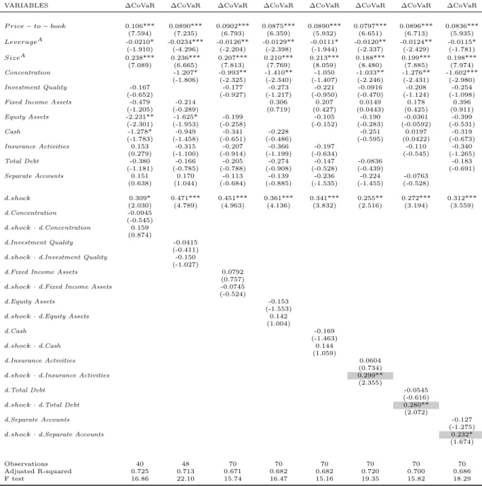
In addition to the robustness check that we conducted by testing the different specifications across 3 different panels we conduct a difference-in-differences (DiD) analysis to check for po-tential endogeneity issues.35 Similar toBrunnermeier et al.(2012), we test the robustness of our findings around Lehman’s filing for bankruptcy and subsequent AIG bailout.36 _{Since Lehman’s}

failure came as an exogenous shock, it represents a good candidate for a natural experiment.37 We adopt the following strategy for the DiD analysis: we run regressions using the same specifications as in equation (4) and we test single variables around the Lehman shock, i.e. systemic risk contribution in 2007 vs 2008, balance sheet items and proxies in 2006 vs 2007. In particular, we construct dummy variables for each of the relevant variable, i.e. Concentration, Investment Quality,Fixed Income Assets,Equity Assets,Cash,Insurance Activities,Total Debt and Separate Accounts.38 The model is the following:

SRi=β0+β1·P rice−to−booki+β2·Leveragei,A/L+β3·Sizei,A/L+

X

j6=z

βj·Xji+ (5)

δ0·d.shock+δ1·d.Xz+δb·d.shock·d.X_z+i (6)

in which thed.shockis a dummy variable which takes value 0 for 2007 and value 1 for 2008 (pre-and post-shock period) (pre-and the d.Xz is a dummy that represents the control (or non-treated

group) and the treatment group respectively. We specify 8 treatment groups, 1 for each relevant

35_{In the panel regressions we use a time lag between dependent and independent variables: theoretically such}

temporal mis-match should shelter our analysis from endogeneity or reverse causality issues.

36_{For further details on the applied DiD methodology, see, for instance,}_Meyer₍₁₉₉₅_{) and}_{Angrist and Krueger}

(1999). For a more didactic contribution, seeWooldridge(2010).

37_{AIG was bailed out by the U.S. Government a day after Lehman’s bankruptcy filing.} 38

We neglectPrice-to-book,LeverageandSizenot because we neglect their importance, but because they have been substantially analyzed in previous work, see for instanceBrunnermeier et al.(2012) for banks and (Bierth et al.,2015) for insurers.

(21)

variable: we divide the observations into 2 groups, above and below the median and assign value 0 and 1 depending on the expected sign of the variable. Table 13 provides an overview of the treatment variables.

Tables14-17report the results of the DiD around the Lehman bankruptcy and AIG bailout: the coefficient of interest is of course the interaction term (δb) between the shock dummy and

the control group. The striking result of such robustness check is that, Insurance Activities, Total Debt andSeparate Accounts appear to be statistically and economically significant deter-minants of systemic risk, although not uniformly for the 2 measures: in fact,Separate Accounts are statistically insignificant for the ∆CoVaR. This confirms our hypothesis that the capital structure, i.e. the liability side, is the key driver of systemic risk in insurance. By contrast Concentration does not display significant coefficients: however, this shall not be taken as a rejectionin toto, rather it deserves further investigation, sinceConcentration is just a proxy and by definition it is an imperfect measure and therefore, measurement errors might be a potential explanation for its insignificance.

5 Conclusion

In the present paper, we propose an analysis of the role of the insurance industry in posing systemic risk and the determinants therein. We divide the analysis into 2 parts: first, we conduct an aggregated industry analysis based on 3 measures of systemic risk on 3 different groups. By doing so, we aim to test the relative systemic risk contribution of the insurance industry vis-`a-vis other industries. In the second part of the analysis, we investigate what are the potential determinants of systemic risk within the insurance industry by focusing on the asset and liability composition of insurers.

Our evidence suggests that financial institutions tend to cause more systemic risk than non-financial institutions; among non-financial institutions, banks pose more systemic risk than insurers, especially after the Lehman bankruptcy. Insurers do cause systemic risk, especially when they engage in non-insurance activities, e.g. banking activities. Furthermore, we find that systemic risk in the insurance industry is mainly driven by the liability side, i.e. the capital structure rather than the asset side: however, on the asset side we find that the level of diversification is also a strong determinant of systemic risk, although further investigation is needed. In addition, traditional variables associated with systemic risk in financial institutions, such as size is of

(22)

importance, whereas price-to-book and leverage seem to play a counterintuitive role. This is however in line with previous findings, which confirm for instance that leverage in insurance is fundamentally different compared to leverage in banking. Results are robust to a set of different specifications, different panels and different econometric methods. Finally, the choice of the time span should shelter the analysis from biases stemming from sample (time-dependency) selection. In conclusion, we provide new evidence on the role of insurers in posing systemic risk, in particular on the role of insurance activities compared to non-insurance activities. Also, we are among the first to provide empirical evidence on the role of diversification in posing systemic risk, which should be further analyzed in future research. Moreover, we are the first to use a European set of companies and to use variables of stock rather than flow: the latter is particularly relevant to show how the stock of the outstanding business drives systemic risk contribution in the insurance industry.

Thus, our research has the potential to provide a significant contribution to shedding ad-ditional light on the debate on systemic risk in the insurance industry as well as insightful indications on how to assess the systemic relevance of insurance companies. This is particularly relevant in the light of the ongoing discussion on the role of SIFIs and on the specific regulations they might be subjected in the future. Furthermore, the present paper could serve as a basis for a theoretical treatment of the systemic risk contribution of the insurance industry, and thereby contribute to deepening the understanding of the underlying economic forces driving systemic risk.

(23)

A

Appendix

A.1 Systemic Risk Measures

A.1.1 The Granger causality test (Billio et al., 2012)

We measure the systemic importance of an institution in terms of the total number of statis-tically significant pairwise connections based on linear Granger causality tests. This approach allows us to infer when equity price movements of an institution influence price movements of another institution over a given period of time. The Granger causality test measures the ability of 2 time series to forecast each other. We can write the system of equations as follows

y_ti₊₁=αiy_ti+βijyj_t +i_t₊₁ (7)

y_tj₊₁=αjyj_t+βjiyi_t+j_t₊₁ (8)

in which coefficientsαi,βij,αj,βji are estimated via linear regression and in which time series

j is said to “Granger-cause” times series iif lagged values of j contain statistically significant information that helps in predictingi.

The causality indicator is defined as follow:

j →i=                1, ifj Granger causesi 0, otherwise 0, forj→j (9)

Equation (9) allows us to calculate a series of indexes based on the total number of significant relations among institutions at a specific point in time.39_The_{Degree of Granger Causality} _thus

represents the fraction of statistically significant relationships over the total number of possible connections among the full sample,

DGC = 1 N(N −1) n X i=1 X j6=i (j →i) (10)

Moreover, we can differentiate between causing and receiving connections which are defined

39

(24)

as follows Out: (j→S)|_DGC≥K= 1 N −1 X i6=j (j→i)|_DGC≥K (11) In: (S →j)|DGC≥K = 1 N−1 X i6=j (i→j)|DGC≥K (12)

Each index represents the contribution of each individual institution. We then calculate industry averages by summing the total number of institutions’ connections across each industry group.

A.1.2 ∆CoVaR (Adrian and Brunnermeier, 2011)

The measure extends the concept ofValue at Risk (VaR) designed for individual institutions to the system as a whole. The CoVaR represent the VaR of a system conditional on institu-tions being in distress. The systemic contribution of an individual institution to the system is computed as the difference between the CoVaR of the institution in distress and the CoVaR in the median state, hence ∆CoVaR. Following Adrian and Brunnermeier(2011), we calculate

(25)

the ∆CoVaR using quantile regressions by setting the median state at the 50 percentile and the distress situation at the 95 percentile. We also include in the regressions a set of 6 state variables Mt−1, namely market volatility, liquidity spread, changes in the short-term interest

rates, the slope of the yield curve, credit spreads and total equity returns, using 1 week lag. Estimations are based on the following equations

X_ti =αi+γiMt−1+εit (19)

X_tS =αS|i+βS|iX_ti+γS|iMt−1+εS_t|i (20)

wherei represents the individual institution and S is the index representing the set of institu-tions under consideration. The predicted value from the regressions are then plugged into the following equation to obtain both the VaR of the individual institution and consequently the CoVaR

V aRi_t(q) = ˆα_qi + ˆγ_qiMt−1 (21)

CoV aR_ti(q) = ˆαS|i+ ˆβS|iV aRi_t(q) + ˆγS|iMt−1. (22)

Finally, the contribution of each institution to the system is calculated as follows:

∆CoV aRi_t(q) =CoV aRi_t(5%)−CoV aRi_t(50%) = ˆβS|i(V aRi_t(5%)−V aRi_t(50%)) (23)

We then distinguish between 3 cases: 1) intra-industry: X_tS = P j6=iw j t−1·r j t P j6=iw j t−1 (24)

withw=market capitalization,r= return,j= i’s industry group,

∆CoV aRintra-industry_t |i = 1 N N X i Φ−1(0.5)∆CoV aRintra-industry_t_→_t₊_h |i (25)

(26)

2) other industries: X_tS = P jw j t−1·r j t P jw j t−1 (26)

withw=market capitalization,r= return,j= excluding i’s industry group,

∆CoV aRother industries_t |i = 1

N

X

i

Φ−1(0.5)∆CoV aRother industries_t_→_t₊_h |i (27)

wheret→t+h indicates 1 calendar month of daily ∆CoVaR. 3) total system: X_tS = P j6=iw j t−1·r j t P j6=iw j t−1 (28)

withw=market capitalization,r= return,j= total system,

∆CoV aRtotal system_t |i = 1

N

X

i

Φ−1(0.5)∆CoV aRtotal system_t_→_t₊_h |i (29)

wheret→t+h indicates 1 calendar month of daily ∆CoVaR.

Where N represents the number of institutions for each of the 3 groups. In order to avoid correlation biases, i.e. under case 1) and 3), we always exclude institution i from the index representing the reference group.

A.1.3 DMES (Brownlees and Engle, 2012)

The measure is based on the expected loss conditional to a distressed situation (eg. returns being less than a certain quantile): Brownlees and Engle(2012) extend the measure proposed by (Acharya et al.,2010) by introducing a dynamic model characterized by time varying volatility and correlation as well a nonlinear tail dependence. The market model is defined as follows

rmt =σmtmt

rit=σitρitmt+σit

q

1−ρ2_itξit (30)

(27)

whereri is the market return of theithinstitution andσitis its conditional standard deviation,

rm is the market return of the system considered and σmt is its conditional standard deviation,

and ξ are the shocks that drive the system and ρit is the conditional correlation between i

and m. The one period ahead DMES can be expressed as follows

DM ES_it1₋₁(C) =σitρitEt−1(mt|mt< C σmt ) +σit q 1−ρ2 itEt−1(ξit|mt< C σmt ) (31)

whereC is the conditioning systemic event which we assume to be equal to the 95th percentile of the total period market return, i.e. C= Φ−1(0.95)rm.40 The conditional standard deviations

and the conditional correlation are estimated by means of a TARCH and a DCC model respec-tively.41 The tail expectationsEt−1(mt|mt <

C σmt ) and Et−1(ξit|mt< C σmt ) are calculated by means of a non-parametric kernel estimator and are given by the following equations

ˆ Eh(mt|mt< k) = Pn i=1mtKh(mt−k) (npˆh) (32) ˆ Eh(ξit|mt< k) = Pn i=1ξitKh(mt−k) (npˆh) (33) with ˆ ph= Pn i=1Kh(mt−k) n

We then distinguish between 3 cases: 1) intra-industry: rmt = P j6=iw j t−1·r j t P j6=iw j t−1 (34)

withw=market capitalization,r= return,j= i’s industry group,

DM ESintra-industry_t |i = 1 N N X i Φ−1(0.5)DM ES_tintra-industry_→_t₊_h |i (35)

wheret→t+h indicates 1 calendar month of daily DMES.

40

The choice over theV aR0.95of the market allows for a more direct comparison with the estimations of the

∆CoVaR.

41

(28)

2) other industries: rmt= P jw j t−1·r j t P jw j t−1 (36)

withw=market capitalization,r= return,j= excluding i’s industry group,

DM ESother industries_t |i = 1 N N X i Φ−1(0.5)DM ES_tother industries_→_t₊_h |i (37)

wheret→t+h indicates 1 calendar month of daily DMES. 3) total system: rmt = P j6=iw j t−1·r j t P j6=iw j t−1 (38)

withw=market capitalization,r= return,j= total system,

DM EStotal system_t |i = 1 N N X i Φ−1(0.5)DM ES_ttotal system_→_t₊_h |i (39)

wheret→t+h indicates 1 calendar month of daily DMES.

Where N represents the number of institutions for each of the 3 groups. In order to avoid correlation biases, i.e. under case 1) and 3), we always exclude institution i from the index representing the reference group.

(29)

B

Tables

Table 1: Institutions: list of the institutions included in the 3 groups

Banks

Name Ticker Country

HSBC HSBA UK

BANCO SANTANDER E:SCH ES

UBS S:UBSN CH

BNP PARIBAS F:BNP FR

LLOYDS BANKING GROUP LLOY UK

ROYAL BANK OF SCOTLAND RBS UK

BARCLAYS BARC UK

CREDIT SUISSE GROUP S:CSGN CH

BBV. ARGENTARIA E:BBVA ES

DEUTSCHE BANK D:DBKX DE

UNICREDIT I:UCG IT

SOCIETE GENERALE F:SGE FR

STANDARD CHARTERED STAN UK

INTESA SANPAOLO I:ISP IT

NORDEA BANK W:NDA SE

KBC B:KB BE

DANSKE BANK DK:DAB DK

COMMERZBANK D:CBKX DE SVENSKA HANDBKN. W:SVK SE SEB W:SEA SE Insurers ALLIANZ D:ALV DE PRUDENTIAL PRU UK AXA F:MIDI FR

ZURICH INSURANCE GROUP S:ZURN CH

MUNICH RE D:MUV2 DE

SWISS RE S:SREN CH

ING H:ING NL

ASSICURAZIONI GENERALI I:G IT

SAMPO M:SAMA FI

LEGAL & GENERAL LGEN UK

AVIVA AV. UK

AEGON H:AGN ND

MAPFRE E:MAP ES

HANNOVER RE D:HNR1 DE

AGEAS B:AGS BE

RSA INSURANCE GROUP RSA UK

VIENNA INSURANCE GROUP O:WNST AT

SCOR SE F:SCO FR SWISS LIFE S:SLHN CH B ˆALOISE S:BALN CH Non-Financials BRITISH PETROLEUM BP. UK VODAFONE VOD UK NOVARTIS S:NOVN CH NESTLE S:NESN CH GLAXOSMITHKLINE GSK UK

ROYAL DUTCH SHELL H:RDSA UK

TOTAL F:TAL FR ROCHE S:ROG CH ENI I:ENI IT TELEFONICA E:TEF ES SANOFI F:SQ@F FR NOKIA M:NOK1 FI SIEMENS D:SIEX DE ASTRAZENECA AZN UK L’OREAL F:OR@F FR E ON D:EONX DE

BRITISH AMERICAN TOBACCO BATS UK

RIO TINTO RIO UK

LVMH F:LVMH FR

(30)

Table 2: Non-Financial institutions: list of the Non-Financial institutions included in the analysis classified according to GICI classification.

Name Sector Industry Group

BRITISH PETROLEUM Energy Energy

VODAFONE Telecommunication Telecommunication

NOVARTIS Health Care Pharmaceuticals & Biotechnology

NESTLE Consumer Staples Food & staples retailing

GLAXOSMITHKLINE Health Care Pharmaceuticals & Biotechnology

ROYAL DUTCH SHELL Energy Energy

TOTAL Energy Energy

ROCHE Health Care Pharmaceuticals & Biotechnology

ENI Energy Energy

TELEFONICA Telecommunication Telecommunication

SANOFI Health Care Pharmaceuticals & Biotechnology

NOKIA Information technology Technology hardware & Equipment

SIEMENS Industrials Capital Goods

ASTRAZENECA Health Care Pharmaceuticals & Biotechnology

L’OREAL Consumer Staples Households and Personal Products

E ON Utilities Utilities

BRITISH AMERICAN TOBACCO Consumer Staples House Beverage & Tobacco

RIO TINTO Materials Materials

LVMH Consumer Staples Households & Personal Products

DIAGEO Consumer Staples Food & staples retailing

Table 3: Total Return Indexes: descriptive statistics of the Total Return Indexes of the 60 institutions on the time period between January 1996 to December 2013. The upper part reports values at monthly frequency, whereas the lower part reports values at daily frequency.

Monthly Data # Obs. Average Median St.Dev. Min Max

Banks 20 4,319 0.0048 0.0119 0.1189 -1.2447 0.6602

Non-Financial 20 4,320 0.0086 0.0125 0.0808 -0.6628 0.5099

Insurers 20 4,304 0.0046 0.0117 0.1137 -2.0293 0.6745

Full Sample 60 12,943 0.0060 0.0121 0.1058 -2.0293 0.6745

Daily Data # Obs. Average Median St.Dev. Min Max

Banks 20 92,160 0.0002 0.0000 0.0256 -1.0957 0.5495

Non-Financial 20 92,160 0.0004 0.0000 0.0192 -0.4578 0.3226

Insurers 20 92,160 0.0002 0.0000 0.0245 -1.4949 0.3022

Full Sample 60 276,480 0.0003 0.0000 0.0232 -1.4949 0.5495

Table 4: State variables: descriptive statistics of daily data observed on the period between January 1999 to December 2013.

Obs. Average Median St.Dev. Min Max