Semi-supervised and Active Learning Models for Software Fault Prediction

(1)

2015

Semi-supervised and Active Learning Models for Software Fault

Prediction

Huihua Lu

Follow this and additional works at: https://researchrepository.wvu.edu/etd

Recommended Citation Recommended Citation

Lu, Huihua, "Semi-supervised and Active Learning Models for Software Fault Prediction" (2015). Graduate Theses, Dissertations, and Problem Reports. 6117.

https://researchrepository.wvu.edu/etd/6117

This Dissertation is protected by copyright and/or related rights. It has been brought to you by the The Research Repository @ WVU with permission from the rights-holder(s). You are free to use this Dissertation in any way that is permitted by the copyright and related rights legislation that applies to your use. For other uses you must obtain permission from the rights-holder(s) directly, unless additional rights are indicated by a Creative Commons license in the record and/ or on the work itself. This Dissertation has been accepted for inclusion in WVU Graduate Theses, Dissertations, and Problem Reports collection by an authorized administrator of The Research Repository @ WVU. For more information, please contact [email protected].

(2)

for

Software

Fault

Prediction

Huihua

Lu

Dissertation

submitted

to

the

Benjamin

M. Statler

College

of

Engineering

and

Mineral

Resources

at

West

Virginia

University

in

partial

fulfillment

of

the

requirements

for

the

degree

of

Doctor

of

Philosophy

in

Computer

Engineering

Bojan

Cukic,

Ph.D.,

Chair

Mark

Culp,

Ph.D.

Afzel

Noore,

Ph.D.

Donald

Adjeroh,

Ph.D.

Vinod

Kulathumani,

Ph.D.

The

Lane

Department

of

Computer

Science

and

Electrical

Engineering

Morgantown,

West

Virginia

2015

Keywords:

software

quality

assurance,

software

fault

prediction,

semi

‐

supervised

learning,

active

learning,

software

metrics,

dimension

reduction

Copyright

2015

Huihua

Lu

(3)

Semi

‐

Supervised

and

Active

Learning

Models

for

Software

Fault

Prediction

Huihua

Lu

As software continues to insinuate itself into nearly every aspect of our life, the quality of software

has been an extremely important issue. Software Quality Assurance (SQA) is a process that ensures

the development of high-quality software. It concerns the important problem of maintaining,

monitoring, and developing quality software. Accurate detection of fault prone components in

software projects is one of the most commonly practiced techniques that offer the path to high quality

products without excessive assurance expenditures. This type of quality modeling requires the

availability of software modules with known fault content developed in similar environment.

However, collection of fault data at module level, particularly in new projects, is expensive and

time-consuming. Semi-supervised learning and active learning offer solutions to this problem for learning

from limited labeled data by utilizing inexpensive unlabeled data.

In this dissertation, we investigate semi-supervised learning and active learning approaches in the

software fault prediction problem. The role of base learner in semi-supervised learning is discussed

using several state-of-the-art supervised learners. Our results showed that semi-supervised learning

with appropriate base learner leads to better performance in fault proneness prediction compared to

supervised learning. In addition, incorporating pre-processing technique prior to semi-supervised

learning provides a promising direction to further improving the prediction performance. Active

learning, sharing the similar idea as semi-supervised learning in utilizing unlabeled data, requires

human efforts for labeling fault proneness in its learning process. Empirical results showed that active

learning supplemented by dimensionality reduction technique performs better than the supervised

learning on release-based data sets.

(4)

List of Figures

3.1 FTF algorithm . . . 22

3.2 FTcF algorithm. . . 23

3.3 Convergence plot on PC3(10%labeled set used).. . . 35

3.4 Convergence plot on PC3 with the measure of PD(10%labeled set used). . 36

3.5 Results of FTF algorithm on PC3(the numbers of modules initially labeled at 2%, 5%, 10%, 20%, 50% are 31, 78, 156, 313,782 respectively) . . . 37

3.6 Results of FTcF algorithm on PC3(the numbers of modules initially la-beled at 2%, 5%, 10%, 20%, 50% are 31, 78, 156, 313,782 respectively) . . 38

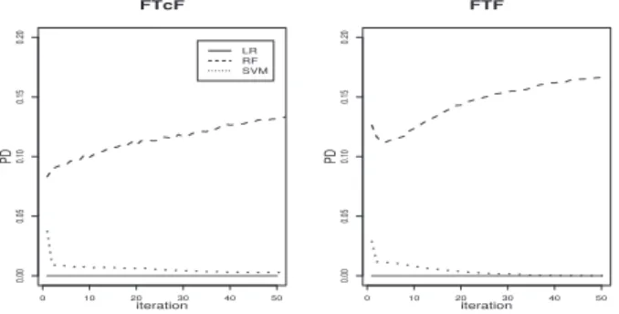
3.7 Results of FTF algorithm on four data set with threshold=0.5. . . 38

3.8 Results of FTcF algorithm on four data set with threshold=0.5.. . . 39

4.1 Dimension Reduction based FTcF Algorithm . . . 46

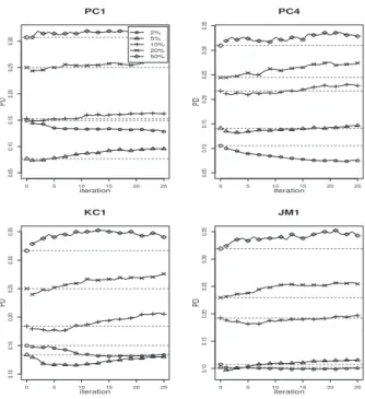
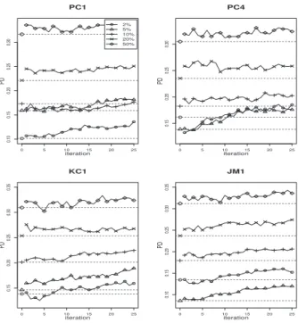
4.2 Performance plots for PC4 project. . . 48

5.1 Active learningn process . . . 58

5.2 Comparison of two active learning sampling strategies with supervised learning approach. 10-cross-validation is used to evaluate the prediction performance of trained models at each iteration. . . 59

5.3 Diagram of the Adaptive Fault Prediction process. . . 60

5.4 Performance of AFP for 5% of initially labeled modules. . . 64

5.8 Comparison between AFP approach and supervised learning. Both use Naive Bayes classifier with varied sizes of labeled data used in training. . 69

6.1 Comparison of different feature selection techniques with active learning using Eclipse 2.0 packages for training and 2.1 for evaluation. . . 73

6.2 Comparison of Euclidean distance vs. RF similarity in multidimensional scaling (MDS) on Eclipse release 2.0. The plus sign represents defective modules, the minuses represent defect-free modules(at package level).. . . 75

6.3 Comparison of Euclidean distance vs. RF similarity in multidimensional scaling (MDS) on Eclipse release 2.0. The plus sign represents defective modules, the minuses represent defect-free modules(at file level). . . 75

6.4 Defect prediction in release 2.1 from 2.0 (Eclipse - packages). . . 82

6.5 Defect prediction in release 3.0 from 2.1 (Eclipse - packages). . . 82

6.6 Defect prediction in release 3.0 from 2.0 and 2.1 (Eclipse - packages) . . . 83

6.7 Defect prediction in release 2.1 from 2.0 (Eclipse - files) . . . 83

6.8 Defect prediction in release 3.0 from 2.1 (Eclipse - files) . . . 84 vi

(8)

6.9 Defect prediction in release 3.0 from 2.0 and 2.1(Eclipse - files) . . . 84

6.10 Defect prediction in release 1.4 from 1.2 (Camel) . . . 87

6.11 Defect prediction in release 1.6 from 1.4 (Camel) . . . 87

6.12 Defect prediction in release 1.3 from 1.4 (Ant). . . 88

6.13 Defect prediction in release 1.5 from 1.6 (Ant). . . 88

(9)

List of Tables

3.1 Datasets used in this study . . . 25

3.2 Number of modules in initially labeled data set . . . 28

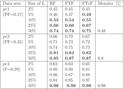
3.3 Comparison between our results and Menzies’s results with Probability of Detection(PD) at specified PF . . . 40

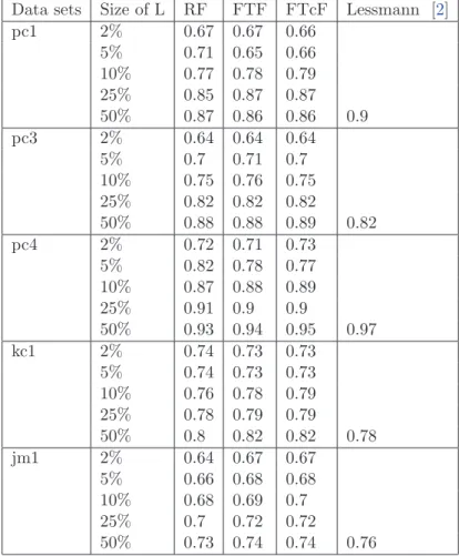
3.4 Comparison between our results and Lessmann’s results with Area under ROC curve(AUC). . . 41

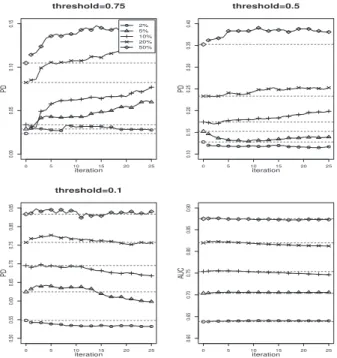
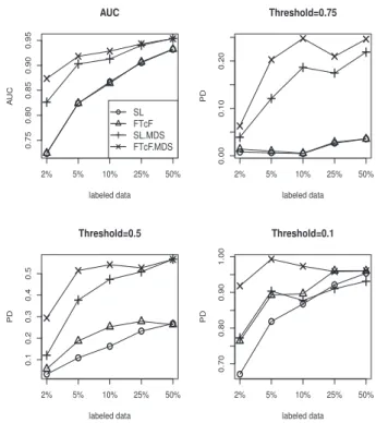
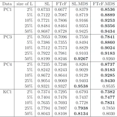
4.1 AUC for the four data sets . . . 49

4.2 PD with threshold=0.75 for the four data sets. . . 50

4.3 PD with threshold=0.5 for the four data sets . . . 51

4.4 PD with threshold=0.1 for the four data sets . . . 51

4.5 One way ANOVA test for PD(threshold= 0.5) at 2% labeled data . . . . 52

4.6 P-value of ANOVA test on varied size of labeled data for all performance measures. . . 52

4.7 Significance comparison of PD(0.5) . . . 52

4.8 Significance comparison of PD(0.1) . . . 52

4.9 Average decrease in AUC measure. . . 53

4.10 Average percent decrease in PD measure (Threshold is 0.5). . . 53

4.11 Comparison of results with [1] . . . 54

4.12 Comparison of results with [2] using AUC. . . 55

5.1 NASA software metrics . . . 62

5.2 Number of modules in initially labeled data set . . . 62

5.3 Percentage of change over the iterations of adaptive learning procedure. . 67

6.1 Software data sets . . . 76

6.2 Metrics in Eclipse data set. . . 77

6.3 Metrics in Camel and Ant data sets . . . 77

6.4 One way ANOVA test for AUC measures at 10th iteration, when defects in release 2.1 are predicted from 2.0 . . . 90

6.5 P-values by ANOVA test, when defects in release 2.1 are predicted from 2.0 (package level) . . . 90

6.6 Post-hoc test for performance differences between the six active learning approaches at package level (1 :M DS Act,2 :M DS rand,3 :IG Act,4 : IG rand,5 :Act,6 :Rand). “X_{” stands for statistically significant} dif-ference between two approaches. “x” stands for no signisficant difference detected between the two approaches. . . 90

(10)

6.7 Post-hoc test for performance differences between the six active learning approaches at file level (1 : M DS Act,2 : M DS rand,3 : IG Act,4 :

IG rand,5 :Act,6 :Rand). “X_{” stands for statistically significant}

dif-ference between two approaches. “x” stands for no signisficant difference

detected between the two approaches. . . 91

7.1 Run-time (minutes) of semi-supervised learning when random forest is used as base learner . . . 99

D.1 Performance comparison, from release 2.0 to 2.1 for Eclipse packages . . . 112

D.2 Performance comparison, from release 2.1 to 3.0 for Eclipse packages.. . . 112

D.3 Performance comparison, from releases 2.0 and 2.1 to 3.0 for Eclipse pack-ages. . . 113

D.4 Performance comparison, from release 2.0 to 2.1 for Eclipse files. . . 113

D.5 Performance comparison, from release 2.1 to 3.0 for Eclipse files. . . 114

D.6 Performance comparison, from releases 2.0 and 2.1 to 3.0 for Eclipse files. 114 D.7 Performance comparison, from release 1.2 to 1.4 for Camel. . . 115

D.8 Performance comparison, from release 1.4 to 1.6 for Camel. . . 115

D.9 Performance comparison, from release 1.3 to 1.4 for Ant. . . 116

(11)

Introduction

1.1 Software Fault Prediction Problem

As software continues to insinuate itself into nearly every aspect of our life, the qual-ity of software has been an extremely important issue. Software Qualqual-ity Assurance (SQA) consists of activities that ensure the development of high-quality software. It encompasses the development and implementation of methods and processes for quality software, regardless of the underlying software development model being used.

To ensure high quality products, software engineers need undertake significant efforts to ensure that software functions are intended while inspecting the risks of vulnerabilities that could bring harm to the end user. Software quality inspection and improvement can be detecting faulty software modules and reducing the number of faults occurring during system operations. A software fault usually refers to a defect or a flaw in an executable product that can cause system failures during operation. Faults in software systems are major problem that need to be resolved. Software module is the lowest level of software for which we have data, for example, java method or class.

It is critical to detecting where fault hides, as it allows verification and validation ex-perts to concentrate their time, efforts, and resources on the potentially problematic modules under development, thus enables Verification and Validation (V&V) activities more effective [3–6]. On the other hand, learning the pattern how faults hide in code helps software engineering improve their design or development in the future project or release. Software fault prediction can identify faults in the current code base, but also warns about future fault-prone areas.

(12)

Over the past years, software fault prediction problem has been an important area of research [7–11]. Given the shorter development and release life cycles, accurate detec-tion of software fault relies increasingly on automated techniques. Machine learning approaches are nature solutions to this type of problem. In a classic machine learning procedure, a predictive model can be trained to form a set of learning rules or patterned structures using training data set, such as historical software modules from previous releases where fault contents are known. The trained model can be then used to esti-mate the fault content of modules currently developed, for example, modules in a newly developed subsystem or in an upcoming project release. Depending on the learning problem, machine learning can be narrowed down into two categories, regression based methods and classification based methods. Target variable refers to ‘response’ variable in statistical language, or ‘label’ in machine learning literature. For regression problem, the target variable can be the number of faults associated with each software module. For classification problem, the target variable is a binary variable, fault proneness (fp) or non-fault proneness (nfp). Predicting the exact amount of faults is too risky, especially in the early development stage when only little information is available. Classifying software intofp ornfp can be more general and reliable. Throughout this dissertation, we focus on the binary classification problem in software fault prediction.

Besides the target variable, an important element in software fault prediction problem is the software metrics, or so-called features in machine learning. Most widely used software metrics includes static code metrics, Object-Oriented (OO) metrics, development process metrics, complexity metrics of modules, network based metrics and many others. The basic idea behind using software metrics is that, for example, more complex the code is more likely to have faults, or a software component is likely to be fault prone if it is similar to other faulty components in code structure or code complexity. Software metrics, for example the static code metrics, can be obtained using automated data collection tools. Typically, software metrics together with their fault contents form the basis of software fault prediction learning data, or training data.

For binary classification problem, software fault prediction models can be assessed using confusion matrix based criteria. The most widely used are accuracy, recall, precision, F-measure, G-mean, or the more recently used AUC measure. In addition, other criteria are also important when deploying fault prediction models in a development environ-ment, including ease of use, computational efficiency, or model comprehensibility.

(13)

1.2 Machine Learning in Software Fault Prediction

Software fault prediction models have been studied since 1990s until now. There have been numerous efforts of applying various types of approaches in software fault prediction problem. Many of them aim to propose approaches to allocate limited SQA resources in a cost effective manner by utilizing machine learning approaches [12–14].

Machine learning practitioners have used unsupervised learning approaches and super-vised learning approaches to estimate the fault contents of software modules, depending on whether labels are available or not in training data. Learning approaches with given labels in the training data set refers to supervised learning. Learning with no labels in the training data set refers to unsupervised learning. Both are important learning branches in machine learning and have been widely employed in software fault predic-tion problem. Intuitively, unsupervised learning approaches are good choices for new developed system which has no previous subsystem or release[15,16], while supervised learning approaches are preferred when the previous subsystem or releases are tested and the corresponding fault contents are obtained[17–20].

In unsupervised learning setting, fault prediction models are built based on the natural structure and distribution of the data points. K-mean and hierarchical clustering are popular unsupervised learning approaches to software fault prediction practitioners. The underlying assumption is that software modules are likely to be labeled the same if they are closely connected to each other or highly grouped together. After the clustering analysis, software experts can label the clusters as eitherfpornfpwithout inspecting the modules one at a time. This eases the labeling task and also saves budget consumed on labeling for each module. This could be significantly important in software development, especially when the software delivery date is urgent and the budgets are very limited. The challenge for unsupervised learning approaches is that the performance of the fault prediction is highly affected by the violation of the density (clustering) assumption, especially, for the situation when the data is strongly imbalanced or the clusters of minority class and majority class are significantly overlapped.

In supervised learning setting, software modules together with their fault contents form the training data set and the trained models can be used to predict fault contents of software modules currently under development. Logistic regression, Naive Bayes, tree-based methods, k-nearest neighbors and support vector machines are commonly used supervised learning approaches. The assumption for supervised learning approaches is that modules in training set and test set are from the same data space. Usually, super-vised learning can provide relatively better performance in fault prediction comparing to unsupervised learning as it fits model with given fault contents. They thus are more

(14)

preferred in practice. However, to ensure high accurate in prediction supervised learning requires a reasonably large set of labeled modules (training set). The more fault contents in the training set the more accurate the trained model. A small set of fault contents will probably mislead the training and bias may arise. This requirement could be hard to meet the development schedule is tight or the budget is limited.

1.3 Practical Problems in Software Fault Prediction

Despite years of researches, the study of software fault prediction seems to have reached a plateau. According to recent studies, the probability of detection (PD) (71%) of fault prediction models may be higher than PD of software reviews (60%) if a robust model is built [21]. In this section, we discuss the practical problem or limits that causes such plateau.

1.3.0.1 Limited Fault Data

To build a desirable predictive model, it requires the training data set, i.e., software fault data as large as possible. Most of the past studies in literature assume that there are enough fault data to build the prediction models. Literature in the field indicates that researchers typically utilize at least 50% of software modules for training[1, 22]. However, sometimes we cannot have enough fault data to build accurate models. For example, a new project may have no previous release. On the other hand, labeling large amount of modules consumes time and human resources, which leads to a higher developing budget. This is problematic for most learning approaches, but particularly weighs in on supervised learning approaches.

1.3.0.2 Imbalance in classes

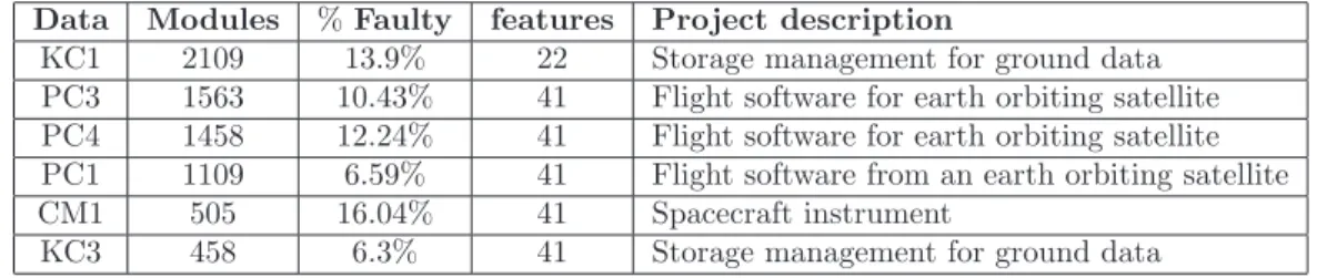
One characteristic of software fault data is that the amount of faulty modules is usually smaller than that of non-faulty modules. Sometimes, such imbalance can be significant. Part of experimental data used in our study are software projects from PROMISE repos-itory, which are very typical examples reflecting the imbalance problem of software fault data (Table3.1). Like most imbalance data prediction problem, the interest of study is on the “rare” class - the fault proneness class. Unfortunately, most commonly used clas-sification approaches are designed to minimize the overall error rate rather than paying particular attention on the “rare” class[23]. Thus they may not work well for imbalance

(15)

data prediction problem. As a consequence, the effectiveness of predictive approaches can be vague if invalid performance measures are used.

1.3.0.3 Low quality in software data

Data Quality is another important issue for software fault prediction problem. Data may be low quality for the following reasons. First, a module may be contaminated by noise, that is, either the complexity metrics or the labels associated to modules are inaccurate. Second, a module may be an outlier in the class it belongs to, which is a typical observation or case. An outlier may or may not be contaminated by noise. The third, software data may be considered low quality if it contains missing values. Although several of imputation methods are available, additional bias or noise may be introduced into the data by missing data imputation. Finally, some other quality issues related to predictors could be constant predictors or inconsistent instances [24, 25]. As by now, very few studies report any data-processing scheme prior to fault prediction process.

The goal of our study is to innovate effective predictive approaches to address the limits in traditional predictive methods. Lacking of labeled data such as the limited fault data problem can be referred to as the|L|<<|U|case where the labeled size is significantly smaller than the unlabeled size, where L denotes the set of labeled data and U de-notes the set of unlabeled data. Intuitively, the knowledge stored in unlabeled modules provides information that can achieve better performance for fault prediction. Thus, semi-supervised learning or active learning is an ideal solution to solve such problem due to their ability of incorporating information from unlabeled data.

1.4 Semi-supervised learning in Software Fault Prediction

problem

Semi-supervised learning has received considerable attention in the machine learning literature due to its potentials in reducing the need for expensive labeled data software fault contents. It has proven successful in image recognition, speech recognition, text categorization, protein structure prediction, and many other domains. Semi-supervised learning falls somewhere between supervised learning and unsupervised learning. In fact, most semi-supervised learning approaches are based on the extension of either supervised learning or unsupervised learning approaches. In a semi-supervised learning setting, both labeled and unlabeled data are used as training data set. With the help of unlabeled data the amount of labeled data could be reduced which in turn reduces

(16)

the cost of labeling for training data [26, 27]. The underlying hypothesis for semi-supervised learning is that knowledge stored in unlabeled modules aids in improving the overall performance of classification.

In this section we will give a brief review on the history of semi-supervised learning. There has been a whole spectrum of interesting ideas on how to learn from both labeled and unlabeled data. It should be noted that semi-supervised learning is a rapidly evolv-ing field, and the review is necessary incomplete. Accordevolv-ing to our knowledge, traditional semi-supervised learning algorithms can be roughly classfied into four categories:

1. Generative algorithms (such as EM algorithm [28]);

2. Iterative algorithms (such as self-training and co-training [29,30]); 3. Density based algorithms (such as transductive-SVM [26]);

4. Graph based algorithm [26, 27].

The generative algorithms require the assumption of data distribution prior to learning. It is common to assume that the data is from multivariate normal distribution, so that the prediction of labels turns out to be the problem of estimating the missed parameters of a normal distribution (µ and Σ). The early work of generative algorithm in semi-supervised learning assumes that the complete data comes from a mixture Gaussian distribution. Let a full generative model be p(D|θ) = p(X, Y|θ), thus the generative model for semi-supervised learning is:

P(D|θ) =P(Xl, Yl, Xu|θ) = X

Yu

p(Xl, Yl, Xu, Yu|θ) (1.1)

where θ = {w, µ,Σ}with Gaussian model p(x, y|θ) = p(y|θ)p(x|y, θ) =wyN(x;µy,Σy.

The goal is to findθto maximizeP(D|θ). Theθcan be solved using maximum likelihood estimation (MLE). For simplicity, consider binary classification problem using MLE, the labeled data has: logp(Xl, Yl|θ) =

l P

i

logp(yi|θ)p(xi|yi, θ). For labeled and unlabeled

The Expectation-Maximization(EM) algorithm is a nature solution to find the optimum. Typically, EM algorithm contains two steps - E-step and M-step. The algorithm starts

(17)

from MLEθ by calculatingθ={w, µ,Σ}on(Xl, Yl). At E-step, the algorithm computes

the expected label p(y|x, θ) = Pp(x,y|θ)

j

p(x,yj|θ) for all x∈ Xu. At the M-step, the algorithm

updates MLEθwith (now labeled)Xu. This procedure repeats the E and M steps until

it converges to a local maximum of θ. Generative semi-supervised learning approaches are in a clear and well-studied probabilistic framework. It can be extremely effective if the model is close to correct. Unfortunately, it is often difficult to verify the correctness of the model assumption. The classification performance may be bad if generative model is wrong.

Unlike generative models, iterative semi-supervised learning algorithms, also called boot-strapping algorithms, do not reply on the knowledge of data distribution. They are ba-sically wrapper methods that apply to existing classifiers. Self-training and co-training are two representatives in this category. The earliest self-training algorithm is called Yarowsky algorithm, which becomes widely known in computational linguistics. Later versions of self-training algorithms are about variants of the Yarowsky algorithm. The Yarowsky algorithm contains two loop. The inner loop is a supervised learning algorithm and called as base learner, consisting of a list of decision rules - If instance xcontains featuref, then predict label j. The base learner selects those rules whose precision on the training data is highest. The Outer loop of self-training is given a seed set of rules to start with. In each iteration, it uses the current set of rules to assign labels to unlabeled data. Then, it selects those instances on which the base learners predictions are most confident. It then calls the inner loop to construct a new classifier and the cycle repeats. Abney has introduced a modified Yarowskey algorithm which differs to the original one in two points: 1) once an unlabeled example gets labeled it stays labeled; 2)the labeling threshold is fixed to be 1/L. In his study, he showed that the original Yarowsky algorithm aims to minimize an objective function. They proposed several variants of Yarowsky algorithm based the difference of objective function. The object function is the cross entropy between the prediction distribution of the model and the labeling distribution over all instances. For labeled instances the entropy of the labeling distribution is zero. Minimizing the objective function forces unlabeled data to be labeled, and forces the model to maximize the likelihood of the (old and newly) labeled data.

In contrast to self-training which iteratively trains a single base learner, co-training requires data attributes to be naturally separated into two views that are conditionally independent given the target label. It is showed that the classifier trained on one view has low generalization error if it agrees on unlabeled data with the classifier trained on the other view. There are also studies to extend two views into multi-views.

(18)

The main assumption for self-training and co-training is that the confidence prediction by base learner(s) is correct. That says both algorithms heavily rely on the base learner. This also implies that early mistake in iterative semi-supervised learning could reinforce themselves.

Next category of semi-supervised learning is density-based algorithm. The assumption regarding density-based algorithms is that the data can be naturally grouped into clus-ters according to the classes they belong to. Given the clustering assumption of the density-based algorithms, the semi-supervised learning problem can be viewed as the maximizing margin problem, i.e., the optimizing marginal technique based algorithms. With the rising popularity of support vector machine, transductive SVMs emerge as an extension of standard SVMs to semi-supervised learning. Transductive SVMs, also called as semi-supervised SVMs or S3VMs, is a method to improve the generalization accuracy of SVMs by using unlabeled data. S3TMs, like SVMs, learn a large marginal plane classifier using labeled training data, but simultaneously force this hyper-plane to be far away from the unlabeled data. More specifically, it aims to find a decision boundary that lies in the region of low density in terms of both labeled and unlabeled data. Therefore, it assumes that the underlying distribution of two classes is such that there is a low-density region between them.

The original S3VMs is based on an iterative algorithm. At the initial iteration, the standard SVMs is used to obtain an initial separating hyper-plane based on the labeled data. Then, pseudo labels are given to the unlabeled samples, which are thus called semi-labeled data. After that, transductive samples chosen from the semi-semi-labeled patterns according to a given criterion are used to define a hybrid training set made up of these semi-samples together with original training samples. The resulting hybrid training set is used at the following iterations to find a more reliable discriminant hyper-plane. This hyper-plane can be derived as follows:

min w,ξl,ξu {1 2w T_w₊_C n X l=1 ξl+C∗ d X u=1 ξu}, s.t.yl[wTφ(xl) +b]≥1−ξl, ξl>0, yu[wTφ(xu) +b]≥1−ξu, ξu>0 (1.3)

where C is the penalty term for misclassification vectorξl, andC∗ is the penalty term

for misclassification vector ξu. φ(.) is any mapping function. yu or ˆyu is the prediction

(19)

In order to handle non-separable training and transductive data, similarly to the SVMs, the slack variables ξl and ξu, and the associated penalty value C and C∗ of both the

training and transductive instances are introduced. d(d < m) is the number of selected unlabeled samples for transductive learning. S3VMs provides a clear mathematical framework and applicable wherever SVMs are applicable. However, S3VMs has difficulty of optimization and can be trapped in bad local optima. On the other hand, it has more modest assumption than generative model or graph-based approaches.

For graph-based semi-supervised learning, the data are represented by a graph, where the edges are labeled with the pairwise similarities. All graph algorithms aim to compute a soft assignment of labels to the nodes of a graph G= (V, E, W), whereV is the set of nodes, E is the set of edges, and W is an edge weight matrix. If edge (u;v) ∈/ E,

Wuv = 0. The assumption of the graph-based semi-supervised algorithms is that the

points connected in a high-density region should belong to the same class.

1.5 Active learning for Software Fault Prediction problem

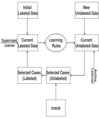
An alternative to semi-supervised learning to address the limited labeled data problem is active learning. The idea of active learning is to improve fault prediction performance by augmenting the training data set with intelligently sampled unlabeled data set. Active learning has many overlaps with iterative semi-supervised learning. For example, active learning requires a base learner iteratively pick the instances from the pool of unlabeled data set in the same way in semi-supervised learning. The key difference between the two learning schemes is that active learning requires the true labels by interacting with an outer oracle, who has expertise to provide ground truth of labels[31]. The general as-sumption behind active learning is that good prediction performance can be achieved by using only “essential data. This characteristic of active learning is desirable in situations where the availability of labeled data is limited.

Active learning approaches vary from different sampling mechanism. There is a class of strategies to sample the data from which to learn. The most popular ones are uncertainty sampling, query-by-committee (QBC), expected error reduction, and density weighted methods [32]. Of these, uncertainty sampling is the most widely used one in machine learning literature. The motivation behind uncertainty sampling is finding unlabeled instances that contain most uncertainty, and use them to clarify the decision boundary. One simplest strategy is to query the instances about which it is least confident how to label. This approach is straightforward for probabilistic learning models. For example, when using a probabilistic model for a binary classification problem, the instances with

(20)

most uncertainty are those with posterior probability closest to 0.5 typical decision cutoff for binary classification with balanced class sizes.

For multi-class problem this least confident criterion only considers information about the most probable label. It “throws away” information about the remaining label distri-bution. To correct for this shortcoming, a more general uncertainty sampling strategy is to use entropy as an uncertainty measure. In this case, one can consider it as selecting instances that maximize the Shannon entropy:

H(y|x) = arg max

x − X

i

P(yi|x)logP(yi|x), (1.4)

where H(x) is the uncertainty measurement function based on the entropy estimation of the classifier’s posterior distribution. P(yi|x) is the posteriori probability. For binary

classes, both least confidence and entropy-based strategy reduce to be equivalent. In our case,y∈ {0,1}where 1 stands for defect prone packages and 0 stands for not defect prone packages. The highest uncertainty score implies that the current learner has the least confidence on its classification of this unlabeled component, thus should be selected first.

The QBC method construct an ensemble of learners induced over labeled data and request labels for instances in unlabeled data set for whose class ensemble members most disagree. This method is inspired by computational learning theory, that is, each committee member may be viewed as a hypothesis consistent with the instances in labeled data set. Acquiring a label for an instance about which two or more hypotheses disagree can be seen as a means of explicitly shrinking the version space, comprising of the hypotheses consistent with labeled data set.

Expected error reduction is decision-theoretic approach, which aims to measure not how much the model is likely to change, but how much its generalization error is likely to be reduced. Instances in unlabeled data set that directly minimize the expected model prediction error should be archived by acquiring a label. This expectation can be computed using the current model. Expected error minimization is appealing because it explicitly maximizes the prediction accuracy. However, in terms of software fault prediction, this type of approaches could be problematic, due to the accuracy is not a suitable performance measure for imbalance class problem in fault data.

Density-weight active learning is a relatively new approach in this subject. The idea behind is that informative instances should not only be those, which are uncertain, but also those which are representative of the underlying distribution. For example, one can query instances by maximize following equation:

(21)

arg max x φA(x)×( 1 U X u sim(x, x(u)))β, (1.5) where φA(x) represents the informativeness of xaccording to a learner A. The second

term weights the informativeness of xby its average similarity to all other instances in the vector space of unlabeled data, subject to a parameter β controlling the relative importance of the second term, i.e., theweights. Density-weighted active learning varies when different learners ofAor different similarity approachessimare used.

In this dissertation we investigate the uncertainty-sampling active learning for software fault prediction problem considering that it is straightforward for probabilistic learning models. We will come back to this with detail in chapter 5.

1.6 Outline

The outline of this proposal is as follows. Chapter 2 provides a literature review for software fault prediction problem. In Chapter 3, we present experimental results of investigating semi-supervised learning in SFP problem. Chapter 4 extends the similar experiments using semi-supervised learning approach with supplemented by dimensional reduction technique. In chapter 5, we present our experiments using active learning approaches. In Chapter 6, we revisit the active learning to release base software data set. Finally, conclusion of our study and future work are discussed in Chapter 7.

(22)

Literature Review

Software fault prediction involves the identification of software locations what quality assurance efforts should focus on. It is one of the most important research areas in software engineering. Studies regarding on software fault prediction can be dated back to the mid 1970s. Each of these studies used their own unique data, features, and predictive techniques and evaluated their models differently. It is important to study the prior work in order to better understand the assumptions and implications of their work. In this Chapter we discuss the elements in software fault prediction models and review the prior literature in the area essential to understanding the role of machine learning in software fault prediction problem.

2.1 Distribution of Faults in Software Systems

A software fault is defined as flaws or imperfection found within code, which may cause the system or system component to fail to perform as required. Faults can be introduced into code at any phase of the software life cycle. In [33], it was discovered that faults in software product are not uniformly distributed throughout the code by investigating three evolutionary releases of a software product. They claimed that the fault rate increases when parts of the code for a new release are modified or newly developed code is added. [34] stated that nearly half of all faults in their telecommunication software system were related to coding faults, majority of which could have been prevented. A recently study based on data extracted from NASA mission stated that requirement faults, coding faults and data problems are the most common types of software faults [35]. They also suggested that observed common trends in software faults are likely intrinsic characteristics rather than project specific.

(23)

The analysis of fault distribution in the development of software systems is an area of interest to software developer as well as empirical researchers. [36] investigated four basic fault distribution hypotheses on two releases of a large commercial telecommunications system. One of the hypotheses showed that a small number of modules contain the majority of faults, that is approximately 20% of all faults are concentrated in about 80% of the modules which follows the Pareto principle. This observation was replicated and confirmed by [37–39]. Later on by Zhang [40], it was shown that the distribution of software faults can be more precisely described as the Weibull distribution, where they implemented Eclipse data and analyzed the distribution of its faults across models in package level. [41] discussed both Pareto and Weibull distribution and proposed a generalized pareto model to assess software fault distribution. Their results showed that the modified pareto model highly fit to the actual fault data.

Another important hypothesis in [36] concerned the similarities in fault densities within project phases or cross projects. This hypothesis was partly supported by their obser-vation. The same hypotheses are replicated in [42] and [43] which confirmed Fenton’s investigation by revisiting the same four hypotheses on different multi-releases software systems.

2.2 Software Metrics

The size metrics, such as the lines of code (LOC), are widely used prediction metrics that are the simplest and easiest to be extracted. Numerous studies investigated the relationship between size of modules and the number of faults, such as [36, 44, 45]. Some studies directly built linear regression models by using software module size as the predictor and fault count as the response. Others derived models analytically first and then fit the data to validate those models, such as Lipow’s logarithmic model and Cox proportional hazard model [45, 46]. In [47], Koru applied cox models and further pro-viding evidence that there is a power-law relationship between size and fault proneness with the latter increasing at a slower rate. This observation supports their hypothesis that smaller modules are proportionally more fault prone. They thus recommended fo-cusing quality assurance resources on smaller modules, as they are more cost effective, i.e., more faults will be found in the same amount of code. This studies were further confirmed in [48] by the study of four large-scale object-oriented products.

In [36], a hypothesis regarding whether size metrics are good predictors of faults is also tested. Their observation shows that size metrics correlate with the number of faults, but there is no strong evidence that size metrics are a good predictor of faults. Limited supporting to the hypothesis was also observed in [42,43].

(24)

In addition to size metrics, complexity metrics such as McCabe’s cyclomatic complexity [49] and Halstead’s metrics [50] are also widely used as fault prediction metrics. Some important studies using complexity metrics can be found in [22, 51, 52]. Fenton and Ohlsso [36] reported that complexity metrics are reasonable predictors but not the best. They observed that both the McCabe and halstead metrics are highly related to each other and to the lines of code. Zhou [53] also noted that size metric has strong con-founding effect on association between complexity metrics and fault proneness and that the explanatory power of complexity metrics is limited.

In a recent study[54], the authors reviewed 106 paper published between 1991 to 2011 and concluded that Object-Oriented metrics and process metrics are more successful at fault prediction than traditional size metrics and complexity metrics. Their findings are similar to those of Hall’s study [55] for size, complexity and OO metrics, but differ regarding process metrics. In Hall’s paper, they reported that process metrics performed the worst among all metrics.

Although most of the research done in recent years focused on the impact of structural properties and process aspect of software component on fault-proneness, there are a few studies that investigated other types of prediction metrics. For example, Nagappan [56,

57] used code churn together with dependency metrics to predict fault-prone modules. In [58] counted the number of changes done in a module as well as the average age of the code.

2.3 Software Fault Prediction Models

Identifying fault in software components effectively is an economically important activ-ity. Software fault prediction is a well-understood research field and has been studied for more than three decades. There exist a large number of modeling techniques to build fault prediction models in the literature. These techniques include statistical modeling techniques such as discriminant analysis [59–61], regression based models [62–66], and machine learning techniques like Naive Bayes [1, 67, 68], random forest [13, 69–71], C4.5 [12, 72, 73], neural network[74–78], and many others[79–85]. In [54], a system-atic review on modeling techniques according 106 papers published from 2000 to 2010 indicated that statistical techniques, primarily logistic regression and linear regression, were used in 68% of the studies, while machine learning techniques were used in 24% of the studies. There are only 8% studies focusing on correlation analysis. However, even the large amount of studies, there is still no consensus on which modeling techniques perform the best when individual studies were viewed separately. Some researchers have

(25)

been conducting empirical overview of various software quality prediction techniques and analyze their performance in terms of various software datasets.

Khoshgoftaar and Seliya [72] compared seven fault prediction techniques that were built using a variety of tools. The models were built using different regression and classification trees including C4.5, CHAID, different versions of CART, logistic regression, and case-based reasoning. The techniques were evaluated against each other by comparing a measure of expected cost of misclassification. The differences between the techniques were at best moderate. They explained that the datasets and system characteristics affect the performance of prediction models.

Guo et al. (2004) compared 27 modeling techniques including random forest, logistic regression and other techniques available through the WEKA tool using five projects from NASA repository. The study compared the techniques using five different datasets from the NASA MDP program, and although the results showed that Random Forests perform better than many other classification techniques in terms of accuracy and speci-ficity, the results were not significant in four of the five data sets.

In [86], the authors compared the performance of thirty predictive techniques on two datasets - JEditData and AR3 from PROMISE repository. This study showed that clas-sification via regression technique and LWL performed better than the other techniques. However, this study was inconclusive as it only used two datasets.

Jiang and Cukic [87] claimed that comparison of fault prediction models is a multi-dimensional problem. Their results across multiple software projects as well as perfor-mance measures showed that there was rarely one model that can be proved to be the best for all possible uses in software quality assessment.

Elish and Elish [88] compared SVM against eight other modeling techniques. The mod-eling techniques were evaluated in terms of accuracy, precision, recall and the F-measure using four data sets from the NASA Metrics Data Program Repository. All techniques achieved an accuracy ranging from approximately 0.83 to 0.94. Their results showed that there were some differences, but no single modeling technique was significantly better than the others across data sets.

Vandecruys [89] compared Ant Colony Optimization against well-known techniques like C4.5, support vector machine (SVM), logistic regression, K-nearest neighbor, RIPPER and majority vote. In terms of accuracy, C4.5 was the best technique. However, the differences among the techniques in terms of accuracy, sensitivity and specificity were moderate.

(26)

Lessman [2] tried to benchmark classification techniques for software fault prediction problem. In his study, 22 techniques over 10 public domain datasets from NASA reposi-tory were compared. However, there are no significant performance differences detected among these techniques. He also argued that fault prediction techniques should not be judged on their predictive performance alone, but that other aspects such as com-putational efficiency, ease of use, and especially comprehensibility should also be paid attention to.

Menzies [1] achieved fault prediction performance of pd=71% and pf=25% on NASA projects using Naive Bayes leaner (with logNum filter) as predictive model, but they also admit that the conclusion may not still apply when the data sets are changed. Another study by Menzies [12] also suggested that to select a preferred learner for a particular domain.

Catal and Diri [90] collected 74 software fault prediction papers in 11 journals and several conferences. According to their review, they indicated that machine learning techniques have better features than statistical methods or expert opinion based approaches, and they suggested that the percentage usage of machine learning techniques should be increased. An extension to this study can be found in [91] where Catal investigated 90 software fault prediction papers published from 1990 to 2009 and provided review on each papers in terms of the year the papers published. Current trend in software fault prediction domain was discussed in their paper.

Arisholm [85] compared many data mining and machine learning methods to build pre-dictive models in an industrial setting for a java system. They showed that the choice of predictive techniques has limited impact on the resulting classification accuracy or cost-effectiveness. They argued that fault prediction techniques that are ranked, as the best is highly dependent on the evaluation criteria applied. Thus, it is important that the evaluation criteria should be justified in the context in which the models are to be applied.

Tracy [55] reviewed 208 papers in term of software fault prediction from 2000 to 2010. They illustrated that simple technique, such as Naive Bayes and Logistic Regression perform comparatively well comparing to technique like SVM and C4.5. However, they also claimed that models seem to have performed best where the right techniques have been selected for the right set of data.

D’Ambros [92] provided a benchmark for software fault prediction models using publicly available datasets consisting of several software systems. They presented an extensive comparison of well-known prediction techniques as well as novel approaches. Their results showed that, while some approaches perform better than others in a statistically

(27)

significant manner, external validity in defect prediction is still an open problem, as generalizing results to different context/leaners proved to be a partially unsuccessful endeavor.

Dejaeger [93] investigated 15 different Bayesian Network algorithms and compared them to other popular machine learning techniques in terms of the AUC and H-measure. Their results showed that augmented Naive Bayes could perform similar or better than the commonly used Naive Bayes classifier. They also claimed that the development context is an item, which should be taken into account during modeling selection.

Recently, a new study [94] evaluated 179 machine learning classifiers, arising from 17 families, over 121 data sets. They concluded that “the classifiers most likely to be the best are the Random Forest (RF) versions”. However, they also recognized that the best-performed classifier has no significantly different with the second best - SVM classifier.

2.4 Semi-supervised and Active learning in Software Fault

Prediction problem

To our knowledge, semi-supervised learning has been marginally considered in the field of software fault-proneness prediction. The earliest study is the work from Khoshgof-taar on NASA MDP software projects[95]. In their study, an EM-based semi-supervised learning algorithm was implemented. As we’ve discussed in previous section, the EM algorithm is natural to this problem since one could view the labels of unlabeled in-stances as missing and thus semi-supervised learning can be reduced to be missing data problem. In their study, a case study is presented in which NASA software project JM1 is used as training data for software measurement modeling. A small size of labeled data is randomly selected from JM1, while remaining modules are treated as the unlabeled dataset. The performance of the EM-based semi-supervised algorithm is evaluated with multiple test datasets consisting of other NASA software projects. Their results demon-strated that the semi-supervised learning approach yielded better performance than a decision tree algorithm - C4.5 trained on program modules with known fault proneness data. Unfortunately, unlike random forest,C4.5 has not been identified as one of the top supervised learning algorithms on the MDP data set [2] making this result inconclusive. They also examined the modules remaining in the unlabeled dataset to be noisy from the perspective of data mining. They observed that roughly half of the modules that remain were in common as noisy.

(28)

Another interesting approach is semi-supervised clustering [96]. Unlike in self-training which extends supervised learning into semi-supervised learning, this approach extends traditional unsupervised learning (clustering) into semi-supervised context so that better partitions (or grouping) is achieved with the use of unlabeled data. However, this is not an entirely automated approach and requires software engineering experts in the loop. Semi-supervised clustering improves the performance compared to the corresponding unsupervised learning, but unsupervised learning does not perform as well as supervised learning. Hence, it is not likely that semi-supervised clustering is a good candidate for practical applications.

Catal[97] proposed an artificial immune system based semi-supervised learning approaches. In their proposed approach, a recent semi-supervised learning algorithm called YATSI (Yet Another Two Stage Idea) is used and in the first stage of YATSI, AIRS - Artificial Immune Recognition System - is applied. In addition, AIRS and Random Forest are benchmarked. Their experiments showed that the performance of AIRS based YATSi are comparable with Random Forest algorithm.

Kocaguneli [98] proposed an active learning solution to the problem of software effort estimation which relax the label data requirement. The proposed approach requires at most 40% of the original data and can perform as well as state-of-the-art supervised learners, which require all the available instances and labels. The reduced set of instances that can provide performance values as good as using all the instances is called as the essential content of the dataset.

Guangchun [99] implemented a two-stage active learning algorithm (TAL) for software defect prediction, in which clustering and support vector machine techniques are com-bined. Their results show that the proposed method improves the performance with a moderate labeling effort.

Li[100] proposed a software fault prediction approach which maps ensemble learning, random forest, into semi-supervised learning setting. Three methods of sampling were discussed in this study: random sampling with conventional machine learners, random sampling with supervised learning learner and active sampling with active semi-supervised learning learner. The proposed semi-semi-supervised learning methods - CoForest and ACoForest - then construct defect prediction models based on selected samples. In their CoForest method, random forest is trained using initially labeled modules. Each random tree is then iteratively refined with the original labels and the labels assigned to previously unlabeled modules from the other random trees. When the stop criterion is reached, the majority voting from the ensemble forms the prediction. CoForest is a disagreement-based semi-supervised learning algorithm, which exploits the advantage of both semi-supervised learning and ensemble learning. The ACoForest method extends

(29)

CoForest by actively selecting and labeling some previously unlabeled data from train-ing the classifiers. Their results showed that the prediction models constructed ustrain-ing CoForest and ACoForest can achieve better performance than those using conventional machine learning techniques, such as logistic regression, decision tree and Naive Bayes.

(30)

Semi-Supervised Learning for

SFP problem

3.1 Semi-Supervised Learning approaches

Semi-supervised learning has tremendous practical value. In manay tasks, there is a dearth of labeled data. The labels Y may be difficult to obtain because they require human annotators, special devices, or expensive and slow experiments. Labeling fault data in software development falls in this category. Semi-supervised learning is attrac-tive because it can potentially utilize both labeled and unlabeled data, assuming that information hidden in unlabeled data are useful in term of prediction.

In the past decade, semi-supervised learning has provided a class of classification ap-proaches that can outperform corresponding supervised learning apap-proaches, especially when|L|<<|U |. Of particular note is self-training, which is the simplest and has less restriction on data compared to the others. One can take a supervised approach as base learner and extend it to semi-supervised learning by an iterative procedure. There are different variants of self-training. The classic one is to take the instances with the high confident scores from unlabeled data and then incorporate them (along with the corre-sponding predictions) into the initial labeled data to train a new leaner for subsequent iteration. The procedure repeats until converge or some stop criterion is met.

Yarowsky’s algorithm [101] is the earliest version of such approach in which a simple decision list learner forms the “inner loop”. If instance x contains feature f, then predict label j, and selects those rules whose precision on the training data is highest. The Outer loop of Yarowsky’s algorithm is given a seed set of rules to start with. The initial Yarowsky algorithm is extended with important modifications such as those from

(31)

Abney et al. [102] and Haffari et al. [103]. The former argued that the best threshold could be fixed at 1/n where n is the size of initial labeled data, and an instance must stay labeled once it becomes labeled, but the label may change. The latter provided a general framework together with mathematical analysis on the variants of the Yarowsky’s algorithm.

In this study we investigate two variants of traditional self-training based semi-supervised approaches in fault prone prediction problem: (i) the existing Fitting The Fits (FTF) approach [104] and (ii) a new variation called Fitting The confident Fits (FTcF).

3.1.1 Notation Definition

To begin, let X be the (n+m)×p matrix that denotes the given software data set.

n is the size of labeled set l and m is the size of unlabeled set u. Rows in X are

p-dimensional vectors defined as x, with x ∈ ℜp_{. Specifically,} _X ₌ _{_X

l, Xu}, where

Xl={x1, x2,· · ·, xn}andXu={xn+1, xn+2,· · ·, xn+m}. LetY ={Yl, Yu}be response

variable (or labels) where Yl = {y1, y2,· · ·, yn} and Yu = {yn+1, yn+2,· · ·, yn+m} is

missing or unspecified. The observed labels are binary variables, yi ∈ {0,1}, where 0

denotes non-fault prone (nfp) module and 1 denotes fault prone (fp) module.

Our task with the investigated algorithms is to extend supervised learning into semi-supervised setting. Let φ(.) be any given supervised learner (base learner). Given a set of input-output pairs Dl = (Xl, Yl), the notation φ_Dl(Xu) indicates that the classifier

trained from Dl is used to predict on unlabeled data set Xu. The probability class

estimates (PCEs) for fault prone class, ˆp = P(Y = 1|Xu), are returned. PCEs are a

specific form of confident scores which is generally used in the literature. Commonly, we consider a module as fault prone when ˆp > τ and non fault prone otherwise, where

ˆ

p∈[0,1] andτ is a specified threshold for making the decision.

3.1.2 Fitting The Fits algorithm - FTF

The FTF algorithm provides an interesting variant of traditional Yarowsky algorithm by extending learners from a supervised setting into a semi-supervised setting. It initially sets up the labels for unlabeled data to ensure that both the labeled set and the unlabeled set are labeled, and then a supervised procedure is implemented on the entire data set. The labels for the unlabeled data are gradually updated until a convergence criterion is met. This is different from Yarowsky’s algorithm in which only a subset of unlabeled data is used to train a new classifier at each iteration. Also, FTF can be shown to globally converge which is a property that cannot be achieved with Yarowsky’s algorithm.

(32)

Figure3.1gives the description of the FTF algorithm. The procedure of FTF starts with setting the initial labels for the unlabeled data at the 0thiteration. Specifically, a learner is trained from initial labeled dataD(0)_l = (Xl, Yl), and then the learner is used to predict

the labels for unlabeled data ˆYu(0) = φ D(0)l

(Xu). In the loop, labels for initial labeled

data set are always reset to be original values ˆYk

l =Yl(step 3). The base learner which

is built based on current status of entire data set D(k) = (X,Yˆ(k)_{) is used to predict}

new labels for entire data set ˆY(k+1) ₌ _φ

D(k)(X) (step 4). This cycle continues until

the statuses of labels converge. We observed that the convergence property is sensitive to the use of base learner, which will be discussed later. Note that the predictions of unlabeled data ˆYu(k) are the probability values (PCEs) in the sense that in the loop the

learner trained is regression based.

Algorithm1: Fitting The Fits (FTF) 1: Initialization: ˆY0

l =Yl, ˆYu0=φ_D(0)

l

(Xu), k= 0;

2: loop until convergence*: 3: Yˆk l =Yl 4: Fit ˆY(k+1)₌_φ D(k)(X), whereD(k)= (X,Yˆ(k)) 5: k=k+ 1 6: End loop Figure 3.1: _{FTF algorithm}

3.1.3 Fitting The confident Fits algorithm - FTcF

Next, we discuss another iterative self-training approach that can be considered as a vari-ant of Yarowsky’s algorithm: Fitting The Confident Fits (FTcF). Typically, a learner trained from current labeled data is used to classify the available unlabeled data. Pre-dicted instances from unlabeled data with high confident scores are considered and added to the pool of labeled data set. Both sizes of labeled data and unlabeled data are up-dated due to the migration of instances from unlabeled data to labeled data at each iteration. As the procedure accesses to the end, the size of unlabeled data set goes to be zero, which means that all instances from unlabeled data set are labeled. The main difference between FTcF and Yarowsky’s algorithm is that in Yarowsky’s algorithm se-lected instances, which are used to train new learner are always given back to the pool of unlabeled data set so that the size of unlabeled data never changes. For FTcF, instances added to the pool of labeled data will stay in the pool with the fixed labels. Therefore, the size of unlabeled data decreases until exhausted. Figure 3.2provides the details for FTcF algorithm.

(33)

Compared to the FTF algorithm, which constructs the learner based on all the modules set by giving an initial “guess” to the labels for unlabeled data, FTcF always learns from current labeled data. Typically, in the iterative phase of FTF the labels for unlabeled data set are updated based on the decision rules probabilities from previous iteration. In contrast, FTcF gradually pushes confident modules into labeled data set so that the size of labeled data set is increasing iteration by iteration. More specifically, in FTF it is considered that there is a “better” classifier by repeatedly fitting the predicted labels in unlabeled data set; in FTcF only a small amount of labels with highest confident scores are trusted. Both algorithms need the guidance of initial labeled data at the beginning.

Algorithm2: Fitting The Confident Fits (FTcF)) 1: Initialization: ˆYl=Yl

2: loop until|u| →0: 3: Fit ˆYu=φDl(Xu)

4: Take u′ _{confident cases from} _X

u 5: updating: Xl=Xl+u′,Yˆl= ˆYl+ ˆYu′, and Xu=Xu−u′ 6: End loop Figure 3.2: _{FTcF algorithm} 3.1.4 Base Learner

Both FTF and FTcF procedures share the underlying concept that a supervised learner is trained repeated by using some form of unlabeled data. Basically, the supervised learner plays two important roles in our investigated algorithms: (i) provides initialization for iterative fitting, and (ii) trains new leaner at each iteration. Apparently, a well-chosen base learner can provide effective prediction for initially unlabeled portion of the data set and ensure a good starting point for tracking “better” learners. On the other hand, the ability that a base learner extracts useful information from unlabeled data at each iteration decides the behavior of entire algorithm. Most important, the selected base learner may lead to local or global convergence. Thus, we have to carefully choose the base learner.

In supervised learning literature, there are lots of choices. We have two constraints on the choices of base learner. First, the learner should have competitive performance in the fault prediction domain and its implementation should be available off-the-shelf. Second, it should produce well-calibrated probabilities, i.e., PCEs. In [105], an examination is provided on the relationship between the predictions made by different supervised algorithms and true posterior probabilities. They showed that some learning algorithms they examined, such as random forest and logistic regression, showed little or no bias

(34)

and predicted well-calibrated probabilities. Based on their work, we will explore random forest and logistic regression as supervised base learners. Also, support vector machine are worth for consideration due to their popularity and off-the-shelf status [106].s

• Logistic Regression (LR)

Logistic regression is a standard off-the-shelf approach for building models for binary classification and has been widely used in software fault prediction problem. Let us assume that PCEs are modeled as a function of a linear combination, i.e, ˆ

p = f(Xβ) ∈ [0,1] where f(.) is a link function . For logistic regression, the function is given as f(Xβ) = ₁₊eXβ_eXβ, which is the logistic transform applied to

Xβ. This transformation forces probabilities to be between 0 to 1. Parameters of a logistic regression model are usually estimated using the maximum likelihood method.

• Support Vector Machine (SVM)

Support Vector Machine (SVM) is another popular classification approach which is motivated by the intuitive geometric interpretation of maximizing the margin. When two classes of points can be separated by a hyper-plane, it is natural to use the hyperplane that separates the two classes of points by the largest margin. This amounts to the hard margin support vector machine:

min w,b 1 2||w|| 2 _(3.1) yi(wTφ(xi) +b)≥1,

The goal is to find the hyper-plane described by{w, b}that generates a maximal margin between two classes of points. One can also utilize a mapping functionφ(.) to allow for the linear separation in non-linear classification problem. To allow the misclassification, one can incorporate a penalty vectorξsuch thatξi≥1 indicates

the corresponding point xi is misclassified. This is well known as soft margin

support vector machine.

min w,b,ξ 1 2||w|| 2₊_CX i ξi (3.2) yi(wTφ(xi) +b)≥1−ξi, ξi>0 • Random Forest (RF)