DRO
Deakin Research Online,
Deakin University’s Research Repository Deakin University CRICOS Provider Code: 00113B
Projected changes in wet-bulb globe temperature under alternative climate
scenarios
Citation:
Newth, David and Gunasekera, Don 2018, Projected changes in wet-bulb globe temperature
under alternative climate scenarios
, Atmosphere
, vol. 9, no. 5(187), pp. 1-12.
DOI:
http://www.dx.doi.org/10.3390/atmos9050187
© 2018, The Authors
Reproduced by Deakin University under the terms of the
Creative Commons Attribution Licence
Downloaded from DRO:
atmosphere
ArticleProjected Changes in Wet-Bulb Globe Temperature
under Alternative Climate Scenarios
David Newth1,* and Don Gunasekera2
1 CSIRO Oceans and Atmosphere, Commonwealth Scientific and Industrial Research Organisation, Canberra, ACT 2601, Australia
2 Centre for Supply Chain and Logistics, Faculty of Science, Engineering and Built Environment, Deakin University, Melbourne Burwood Campus, Burwood, VIC 3125, Australia;
don.gunasekera@deakin.edu.au
* Correspondence: david.newth@csiro.au; Tel.: +61-2-6281-8261
Received: 6 April 2018; Accepted: 14 May 2018; Published: 15 May 2018 !"#!$%&'(!!"#$%&' Abstract:The increased levels of Greenhouse Gasses (GHGs) in the atmosphere will result in increased near-surface air temperature and absolute humidity. These two factors increasingly pose a risk of heat stress to humans. The Wet-Bulb Globe Temperature (WBGT) is a widely used and validated index for assessing the environmental heat stress. Using the output from the Coupled Model Intercomparison Project Phase 5 (CMIP5) simulations of the four Representative Concentration Pathways (RCPs), we calculated the global and regional changes in WBGT. Globally, the WBGT is projected to increase by 0.6–1.7 C for RCP 2.6 and 2.37–4.4 C for RCP 8.5. At the regional scale, our analysis suggests a disproportionate increase in the WBGT over northern India, China, northern Australia, Africa, Central America and Southeast Asia. An increase in WBGT has consequences not only on human health but also on social and economic factors. These consequences may be exacerbated in developing economies, which are less able to adapt to the changing environmental conditions.
Keywords:wet-bulb globe temperature; representative concentration pathways; heat stress
1. Introduction
Climate change simulations suggest that the global near-surface air temperature will increase in the future due to the effects of elevated concentrations of greenhouse gases (GHGs) in the atmosphere [1]. The increase in the near-surface air temperature causes changes in other environmental conditions, such as humidity. These combined effects can pose a significant threat not only to economic output and infrastructure but also to human health and well-being through heat stress [2–9]. Heat stress is an individual experience, which is dependent upon two factors: the amount of heat an individual internally generates from the physical activity he/she is undertaking; and the characteristics of the environment governing the heat transfer between the atmosphere (air temperature, humidity, and radiant heat) and the human body. Humans can survive in air temperatures exceeding both skin and core temperatures through the evaporative cooling of their skin. As a result, the use of various meteorological metrics, such as dry air temperature or apparent temperature [2,10], to assess the effect of heat stress on humans can be unreliable [11]. By contrast, the Wet-Bulb Globe Temperature (WBGT) captures the combined effects of air temperature, humidity, wind and radiative forcing on heat transfer between the environment and the human body. As a result, this has become the accepted international standard for the assessment of heat stress [11].
A number of studies have pointed out the relative vulnerability of various regions of the world, including South-East Asia, South-Eastern USA and Northern Australia to heat stress. A study by Dunne et al. [3] demonstrated that labour capacity could be reduced by over 60% during peak summer Atmosphere2018,9, 187; doi:10.3390/atmos9050187 www.mdpi.com/journal/atmosphere
Atmosphere2018,9, 187 2 of 12
months due to heat stress. Dunne et al. [3] also showed that a wider geographical area of the world, including China, Eurasia, Europe, Africa and Latin America, were also vulnerable to heat stress under the Intergovernmental Panel on Climate Change’s (IPCC) RCP 8.5 emissions scenario. Beyond the direct health-related implications, due to the massive reduction in labour capacity, heat stress has significant social and economic implications, particularly for the developing and emerging economies that are dependent upon labour-intensive economic activities and are less able to adapt to the changing environmental conditions.
The latest generation of climate scenario projections indicates that under the RCP 8.5 scenario, the average global near-surface air temperatures will increase by 2.6–4.8 C during the period of 2081–2100 compared to the temperatures in 1986–2005 [1]. The more likely scenarios of RCP 4.5 and 6.0 suggest a warming of 1.1–2.6 C (RCP 4.5) and 1.4–3.1 C (RCP 6.0) compared to the temperatures in 1986–2005. Such an increase in temperature poses significant social, economic and human health risks [1]. Dunne et al. [3] demonstrated that due to the WBGT’s lack of sensitivity to weather-scale events that drive extreme weather and its demonstrated applicability to human health and well-being, this index is a robust metric for the characterisation of the baseline climate conditions represented in the global climate models [3]. Given this background, this paper aims to focus our analysis on the large-scale change in climate that leads to the conditions conducive for heat stress; and to explore the global and regional changes to the Wet-Bulb Globe Temperature patterns as simulated by the latest generation of earth system models with the consideration of alternative scenarios of GHG emissions. The organisation of the rest of this paper is as follows. The methods used and experiments undertaken are described in Section2. The results are presented in Section3. A discussion of the key findings and their implications are presented in Section4. Key conclusions and closing comments are given in the final section.
2. Methods and Experiments
In the present study, we explored the global and regional changes in WBGT under various IPCC GHG emissions pathways. In the following sub-section, we outlined the Davies-Jones method for the calculation of the Wet-Bulb Globe Temperature. After this, we describe the four IPCC emissions scenarios.
2.1. Davies-Jones Method for Calculating Wet-Bulb Globe Temperature
We followed Dunne et al. [3] and used the Davies-Jones [12] method for calculating the Wet-Bulb Temperature from the output of our analysis. We will briefly cover the calculation in the remainder of this subsection. The general form of the WBGT is [6,12,13]:
Twbgt=0.7Twbt+0.2Tg+0.1Ta (1)
whereTwbtis the natural Wet-Bulb Temperature, in C;Tgis the temperature of a 150-mm diameter black globe ( C); and Ta is the air temperature ( C). As summarized in a previous study [13], it is possible to simplify Equation (1). Under shaded and indoor conditions withTg ⇡ Ta, Twbgt becomes [13]:
Twbgt=0.7Twbt+0.3Ta (2)
whereTa =Tre f 273.15, withTre f defined as the absolute air temperature (K) at a reference level of 2 m. As reported in previous studies [3,13], by doing this, we ignore the radiative and extreme daytime components as well as the other weather scale events that drive extreme weather conditions. This makes the above definition of WBGT insensitive. However as pointed out in reference [3], when compared to other heat stress metrics, this insensitivity makes this approach a more robust metric for assessing the baseline climate conditions represented in the global climate and Earth system models that lack the resolution (in space, time and process) to capture the fine-scale weather events [3]. As a result, our estimates reflect an average to lower-limit of WBGT, which can be thought of as the large-scale
Atmosphere2018,9, 187 3 of 12
‘priming’ of the climate against which the finer scale climate, weather and extreme conditions play out. As derived in a previous study [12], the Wet-Bulb Temperature,Twbt, is calculated as:
Twbt=45.114 51489 ✓ qE 273.15 ◆ 3.504 (3) which is the temperature of a parcel of air if it were cooled to saturation (100% relative humidity) by the evaporation of water into it, with the latent heat being supplied by the parcel. It should be noted thatTwbtTg.qEis the equivalent potential temperature (K). This is the temperature that a parcel of air would reach if it continued to be adiabatically lifted to condense all water, before being lowered dry adiabatically to 1000 mbar (see previous study [14] Equation (43)):
qE=Tre f 1000p re f !0.2854(1 0.28⇥10 3w) exp ✓✓3.376 TL 0.00254 ◆ w⇣1+0.81⇥10 3w⌘◆ (4) whereprefis the surface pressure (mbar) at a reference level of 2 m andTL is the lifting condensation temperature (K). This is the temperature at which the relative humidity would reach 100% upon adiabatic lifting, which is defined as (see reference [14] Equation (43)):
TL= ⇣ 1 Tre f 55 ln ⇣rhre f 100 ⌘ /2840⌘+55 (5)
whererhre f is the relative humidity at a reference level of 2 m (0.01% rhre f 100%). We definedw to be the mixing ratio (g kg 1), which can be calculated as:
w= rhre f
100 wsat (6)
andwsat is the saturation mixing ratio (g kg 1):
wsat=621.97p esat
re f esat (7)
whereesat is the saturation vapour pressure (mbar) (derived from reference [14] Equation (9) and reference [15] Equation (15) and Table 1) which is defined as:
esat=exp ✓ 2991.2729 T2 re f 6017.0128 Tre f +18.87643854 0.028354721Tre f +1.7838310⇥10 7T2 re f 8.4150417⇥10 10Tre f3 +4.4412543⇥10 13T4 re f+2.858487ln ⇣ Tre f ⌘⌘ /100 (8)
2.2. Representative Concentration Pathways
The latest generation of the IPCC scenarios, namely the Representative Concentration Pathways (RCPs), are defined as the trajectories of globally averaged radiative forcing at the top of the atmosphere, which culminate in increases of 2.6, 4.5, 6.0 and 8.5 Wm 2, respectively, in 2100 compared to the forcing
in the reference year of 1850 [16]. In principle, each RCP could be achieved by a wide range of emissions scenarios, representing different combinations of the social, economic and technological settings or Shared Socio-economic Pathways (SSPs) [17,18]. The four RCP scenarios span a wide range of actions on the climate change from RCP 8.5, which is effectively a ‘business-as-usual’ scenario resulting in a climate warming of 3.2–5.4 K by 2100, through to RCP 2.6 (RCP 3PD), which is an ambitious mitigation scenario that stabilizes warming at approximately 2 K above the preindustrial levels. The CO2emission
Atmosphere2018,9, 187 4 of 12
trajectories for each scenario is shown in Figure1. In terms of the environmental outcomes, RCP 8.5 results in an atmospheric CO2concentration of >1350 ppm and a radiative forcing increase at the
top of the atmosphere of 8.5 Wm 2CO
2equivalents (CO2e) in 2100 [19]. Currently, the observations
from the Global Carbon Project show that the world’s CO2emissions were tracking above RCP 8.5 before 2015, although this is now tracking below this scenario but above the other RCPs [20]. The two moderate action scenarios of RCP 6.0 [21] and RCP 4.5 [22] lead to atmospheric concentrations of ⇡850 ppm and⇡650 ppm CO2e, respectively, in 2100. The ambitious action scenario RCP 2.6 [23] is a
peak-and-decline scenario, where the radiative forcing reaches⇡3 Wm 2around 2060 and declines to ⇡2.6 Wm 2in 2100 with a corresponding concentration peak of⇡490ppm CO
2e.
Several observations should be made about the RCPs. First, as seen in Figure1, the emissions trajectory for a given RCP is independent of the other RCPs. For example, it can be seen from Figure1
that RCP 2.6 and RCP 4.5 have higher emissions than RCP 6.0 in 2020 and 2040, respectively. This should be taken into account when interpreting the CMIP5 model output, as RCP 2.6 and 4.5 will have higher warming than RCP 6.0 in the earlier years. Second, RCP 2.6 requires negative emissions after 2080 and there is considerable uncertainty as to how the Earth system will respond to the direct removal of CO2from the atmosphere. Finally, the RCP pathway is highly contingent upon
the socio-economic pathway along which society develops, including technology development and deployment, population growth, affluence, resource usage and efficiency and use of energy technology among other adaptation and mitigation settings [17,18]. Although RCP 8.5 is an unlikely outcome given the current emissions trajectory, the analysis of this scenario is included to give the possible range of outcomes that are linked with the possible global temperatures.
Atmosphere 2018, 9, x FOR PEER REVIEW 4 of 12
Wm−2 around 2060 and declines to ≈2.6 Wm−2 in 2100 with a corresponding concentration peak of
≈490ppm CO2e.
Several observations should be made about the RCPs. First, as seen in Figure 1, the emissions trajectory for a given RCP is independent of the other RCPs. For example, it can be seen from Figure 1 that RCP 2.6 and RCP 4.5 have higher emissions than RCP 6.0 in 2020 and 2040, respectively. This should be taken into account when interpreting the CMIP5 model output, as RCP 2.6 and 4.5 will have higher warming than RCP 6.0 in the earlier years. Second, RCP 2.6 requires negative emissions after 2080 and there is considerable uncertainty as to how the Earth system will respond to the direct
removal of CO2 from the atmosphere. Finally, the RCP pathway is highly contingent upon the
socio-economic pathway along which society develops, including technology development and deployment, population growth, affluence, resource usage and efficiency and use of energy technology among other adaptation and mitigation settings [17,18]. Although RCP 8.5 is an unlikely outcome given the current emissions trajectory, the analysis of this scenario is included to give the possible range of outcomes that are linked with the possible global temperatures.
Figure 1. The CO2 Emissions Pathways for the four IPCC RCP scenarios. These emissions scenarios represent a wide cross-section of action to mitigate the climate change from “no action” (RCP 8.5) to very strong action (RCP 2.6). The observations from the Global Carbon Project [20] show that we are currently tracking above the RCPs 6.0–2.6 scenario. RCP Emissions pathways are from references [19,21–23].
2.3. Observations and Coupled Model Projections
The changes in Wet-Bulb Globe Temperature associated with each RCP emission trajectory is based on the output of a multi-model ensemble of the climate and earth system model simulations of history and RCP scenarios for 1860–2100, which contributed to CMIP5 [24]. The models display a wide range of climate sensitivities with Equilibrium Climate Sensitivity (ECS) that range over 2.0– 4.67 K and Transitives Climate Response (TCR) that range over 1.1–2.5 K, which allow the analysis to explore a robust set of climate uncertainties [25]. A list of models used in the study is given in Appendix A, along with the RCPs scenarios used.
2.4. Correcting Model Biases
To assure that the simulated model results were consistent with instrument observations, each scenario used was corrected to the National Center for Environmental Prediction (NCEP) reanalysis [26] for the period of 1948–2013. Following Dunne et al. [3], we corrected the biases in the model output, including (1) biases in the geographic structure of the mean WBGT; and (2) biases in the variability in the extremes around the climatological mean. The bias correction algorithms used in this paper are detailed in reference [3].
Figure 1.The CO2Emissions Pathways for the four IPCC RCP scenarios. These emissions scenarios represent a wide cross-section of action to mitigate the climate change from “no action” (RCP 8.5) to very strong action (RCP 2.6). The observations from the Global Carbon Project [20] show that we are currently tracking above the RCPs 6.0–2.6 scenario. RCP Emissions pathways are from references [19,21–23]. 2.3. Observations and Coupled Model Projections
The changes in Wet-Bulb Globe Temperature associated with each RCP emission trajectory is based on the output of a multi-model ensemble of the climate and earth system model simulations of history and RCP scenarios for 1860–2100, which contributed to CMIP5 [24]. The models display a wide range of climate sensitivities with Equilibrium Climate Sensitivity (ECS) that range over 2.0–4.67 K and Transitives Climate Response (TCR) that range over 1.1–2.5 K, which allow the analysis to explore a robust set of climate uncertainties [25]. A list of models used in the study is given in AppendixA, along with the RCPs scenarios used.
Atmosphere2018,9, 187 5 of 12
2.4. Correcting Model Biases
To assure that the simulated model results were consistent with instrument observations, each scenario used was corrected to the National Center for Environmental Prediction (NCEP) reanalysis [26] for the period of 1948–2013. Following Dunne et al. [3], we corrected the biases in the model output, including (1) biases in the geographic structure of the mean WBGT; and (2) biases in the variability in the extremes around the climatological mean. The bias correction algorithms used in this paper are detailed in reference [3].
3. Results
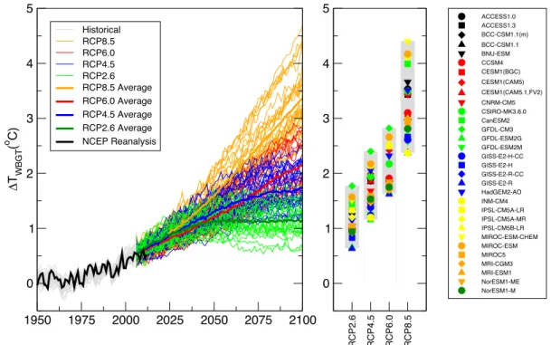
Figure2shows the average annual global change in WBGT during the period of 1950–2100, which is relative to the long-term average between 1948–2010. For RCP 8.5, the global change in WBGT that was averaged over the last decade of this century shows an increase of 2.37–4.4 C, with an ensemble average of 3.36 C. By contrast, the two scenarios with moderate actions on climate change, RCP 6.0 and RCP 4.5, show an increase of 1.6–2.8 C (with an ensemble mean of 2.1 C) and 1.1–2.4 C (with an ensemble average of 1.72 C), respectively. These results suggest that a global moderate action on climate change can have a significant impact on reducing WBGT. Finally, RCP 2.6 shows an increase in WBGT of 0.6–1.7 C (ensemble average of 1.1 C).
The changes in WBGT will not be distributed uniformly across the globe. The regional weather patterns and topography all play a role in influencing the WBGT. Figure3shows the spatial pattern in the maximum monthly mean WBGT.
Atmosphere 2018, 9, x FOR PEER REVIEW 5 of 12
3. Results
Figure 2 shows the average annual global change in WBGT during the period of 1950–2100, which is relative to the long-term average between 1948–2010. For RCP 8.5, the global change in WBGT that was averaged over the last decade of this century shows an increase of 2.37–4.4 °C, with an ensemble average of 3.36 °C. By contrast, the two scenarios with moderate actions on climate change, RCP 6.0 and RCP 4.5, show an increase of 1.6–2.8 °C (with an ensemble mean of 2.1 °C) and 1.1–2.4 °C (with an ensemble average of 1.72 °C), respectively. These results suggest that a global moderate action on climate change can have a significant impact on reducing WBGT. Finally, RCP 2.6 shows an increase in WBGT of 0.6–1.7 °C (ensemble average of 1.1 °C).
The changes in WBGT will not be distributed uniformly across the globe. The regional weather patterns and topography all play a role in influencing the WBGT. Figure 3 shows the spatial pattern in the maximum monthly mean WBGT.
Figure 2. Average global change in WBGT during the period of 1950–2100 compared to the long-term average (1948–2010). For RCP 2.6, the global average WBGT increases by 0.6–1.7 °C (ensemble average of 1.1 °C); RCP 4.5 increases by 1.1–2.4 °C (ensemble average of 1.72 °C), RCP 6.0 increases by 1.6–2.8 °C (ensemble average of 2.1 °C); and RCP 8.5 increases by 2.37–4.4 °C (ensemble average of 3.36 °C).
1950 1975 2000 2025 2050 2075 2100 0 1 2 3 4 5 ∆ TWBGT ( o C) Historical RCP8.5 RCP6.0 RCP4.5 RCP2.6 RCP8.5 Average RCP6.0 Average RCP4.5 Average RCP2.6 Average NCEP Reanalysis RCP2.6 RCP4.5 RCP6.0 RCP8.5 0 1 2 3 4 5 ACCESS1.0 ACCESS1.3 BCC-CSM1.1(m) BCC-CSM1.1 BNU-ESM CCSM4 CESM1(BGC) CESM1(CAM5) CESM1(CAM5.1,FV2) CNRM-CM5 CSIRO-MK3.6.0 CanESM2 GFDL-CM3 GFDL-ESM2G GFDL-ESM2M GISS-E2-H-CC GISS-E2-H GISS-E2-R-CC GISS-E2-R HadGEM2-AO INM-CM4 IPSL-CM5A-LR IPSL-CM5A-MR IPSL-CM5B-LR MIROC-ESM-CHEM MIROC-ESM MIROC5 MRI-CGM3 MRI-ESM1 NorESM1-ME NorESM1-M
Figure 2.Average global change in WBGT during the period of 1950–2100 compared to the long-term average (1948–2010). For RCP 2.6, the global average WBGT increases by 0.6–1.7 C (ensemble average of 1.1 C); RCP 4.5 increases by 1.1–2.4 C (ensemble average of 1.72 C), RCP 6.0 increases by 1.6–2.8 C (ensemble average of 2.1 C); and RCP 8.5 increases by 2.37–4.4 C (ensemble average of 3.36 C).
Atmosphere2018,9, 187 6 of 12
Atmosphere 2018, 9, x FOR PEER REVIEW 5 of 12
3. Results
Figure 2 shows the average annual global change in WBGT during the period of 1950–2100, which is relative to the long-term average between 1948–2010. For RCP 8.5, the global change in WBGT that was averaged over the last decade of this century shows an increase of 2.37–4.4 °C, with an ensemble average of 3.36 °C. By contrast, the two scenarios with moderate actions on climate change, RCP 6.0 and RCP 4.5, show an increase of 1.6–2.8 °C (with an ensemble mean of 2.1 °C) and 1.1–2.4 °C (with an ensemble average of 1.72 °C), respectively. These results suggest that a global moderate action on climate change can have a significant impact on reducing WBGT. Finally, RCP 2.6 shows an increase in WBGT of 0.6–1.7 °C (ensemble average of 1.1 °C).
The changes in WBGT will not be distributed uniformly across the globe. The regional weather patterns and topography all play a role in influencing the WBGT. Figure 3 shows the spatial pattern in the maximum monthly mean WBGT.
Figure 2. Average global change in WBGT during the period of 1950–2100 compared to the long-term average (1948–2010). For RCP 2.6, the global average WBGT increases by 0.6–1.7 °C (ensemble average of 1.1 °C); RCP 4.5 increases by 1.1–2.4 °C (ensemble average of 1.72 °C), RCP 6.0 increases by 1.6–2.8 °C (ensemble average of 2.1 °C); and RCP 8.5 increases by 2.37–4.4 °C (ensemble average of 3.36 °C).
1950 1975 2000 2025 2050 2075 2100 0 1 2 3 4 5 ∆ TWBGT ( o C) Historical RCP8.5 RCP6.0 RCP4.5 RCP2.6 RCP8.5 Average RCP6.0 Average RCP4.5 Average RCP2.6 Average NCEP Reanalysis RCP2.6 RCP4.5 RCP6.0 RCP8.5 0 1 2 3 4 5 ACCESS1.0 ACCESS1.3 BCC-CSM1.1(m) BCC-CSM1.1 BNU-ESM CCSM4 CESM1(BGC) CESM1(CAM5) CESM1(CAM5.1,FV2) CNRM-CM5 CSIRO-MK3.6.0 CanESM2 GFDL-CM3 GFDL-ESM2G GFDL-ESM2M GISS-E2-H-CC GISS-E2-H GISS-E2-R-CC GISS-E2-R HadGEM2-AO INM-CM4 IPSL-CM5A-LR IPSL-CM5A-MR IPSL-CM5B-LR MIROC-ESM-CHEM MIROC-ESM MIROC5 MRI-CGM3 MRI-ESM1 NorESM1-ME NorESM1-M
Atmosphere 2018, 9, x FOR PEER REVIEW 6 of 12
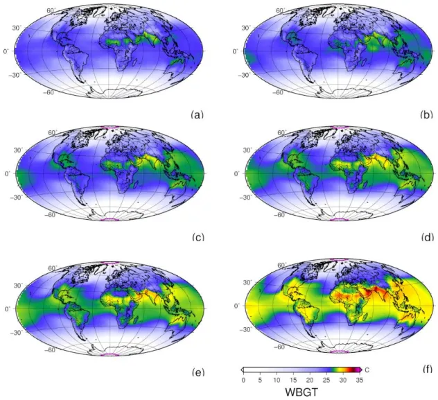
Figure 3. Projected ten-year maximum monthly mean Wet-Bulb Globe Temperature under the Representative Concentration Pathways. In this present study, WBGT is derived from the Wet Bulb Temperature and near-surface air temperature ( ) as a proxy for globe temperature. (a) NCEP reanalysis during the period of 1951–1960; (b) NCEP reanalysis for the most recent decade of 2001– 2010; (c) Projected maximum monthly WBGT for RCP 2.6 for 2091–2100; (d) Projected maximum monthly WBGT for RCP 4.5 for 2091–2100; (e) Projected maximum monthly WBGT for RCP 6.0 for 2091–2100; and (f) Projected maximum monthly WBGT for RCP 8.5 for 2091–2100. For each of the RCPs, the projections are averaged over an ensemble of models from CMIP5 listed in Appendix A. Figures 3 and 4 illustrate the absolute and relative regional changes in the ten-year maximum monthly mean WBGT in the absolute and relative terms, respectively. The human body attempts to maintain a core body temperature of around 37 °C [4–11]. When an individual undertakes physical activity, this creates metabolic heat, which needs to be dissipated to the external environment to avoid the symptoms of heat stress [4–11].
Figure 5 shows the relationship between the metabolic heat created and the cut-off for sustainable WBGT exposure [5]. For points of reference, resting creates around 117 W; moderate labour, such as sustained hand and arm action (hammering) as well as intermittent handling of moderately heavy material, and walking at 3.5–5.5 km/h creates around 297 W; and very heavy labour and intensive activities, such as running, intense shovelling or digging or working with heavy hand tools (e.g., an axe), creates around 522 W [4].
Figure 3. Projected ten-year maximum monthly mean Wet-Bulb Globe Temperature under the Representative Concentration Pathways. In this present study, WBGT is derived from the Wet Bulb Temperature and near-surface air temperature(Tre f)as a proxy for globe temperature. (a) NCEP reanalysis during the period of 1951–1960; (b) NCEP reanalysis for the most recent decade of 2001–2010; (c) Projected maximum monthly WBGT for RCP 2.6 for 2091–2100; (d) Projected maximum monthly WBGT for RCP 4.5 for 2091–2100; (e) Projected maximum monthly WBGT for RCP 6.0 for 2091–2100; and (f) Projected maximum monthly WBGT for RCP 8.5 for 2091–2100. For each of the RCPs, the projections are averaged over an ensemble of models from CMIP5 listed in AppendixA.
Figures3and4illustrate the absolute and relative regional changes in the ten-year maximum monthly mean WBGT in the absolute and relative terms, respectively. The human body attempts to maintain a core body temperature of around 37 C [4–11]. When an individual undertakes physical activity, this creates metabolic heat, which needs to be dissipated to the external environment to avoid the symptoms of heat stress [4–11].
Figure5shows the relationship between the metabolic heat created and the cut-off for sustainable WBGT exposure [5]. For points of reference, resting creates around 117 W; moderate labour, such as sustained hand and arm action (hammering) as well as intermittent handling of moderately heavy material, and walking at 3.5–5.5 km/h creates around 297 W; and very heavy labour and intensive activities, such as running, intense shovelling or digging or working with heavy hand tools (e.g., an axe), creates around 522 W [4].
Atmosphere2018,9, 187 7 of 12
Atmosphere 2018, 9, x FOR PEER REVIEW 6 of 12
Figure 3. Projected ten-year maximum monthly mean Wet-Bulb Globe Temperature under the Representative Concentration Pathways. In this present study, WBGT is derived from the Wet Bulb Temperature and near-surface air temperature ( ) as a proxy for globe temperature. (a) NCEP reanalysis during the period of 1951–1960; (b) NCEP reanalysis for the most recent decade of 2001– 2010; (c) Projected maximum monthly WBGT for RCP 2.6 for 2091–2100; (d) Projected maximum monthly WBGT for RCP 4.5 for 2091–2100; (e) Projected maximum monthly WBGT for RCP 6.0 for 2091–2100; and (f) Projected maximum monthly WBGT for RCP 8.5 for 2091–2100. For each of the RCPs, the projections are averaged over an ensemble of models from CMIP5 listed in Appendix A. Figures 3 and 4 illustrate the absolute and relative regional changes in the ten-year maximum monthly mean WBGT in the absolute and relative terms, respectively. The human body attempts to maintain a core body temperature of around 37 °C [4–11]. When an individual undertakes physical activity, this creates metabolic heat, which needs to be dissipated to the external environment to avoid the symptoms of heat stress [4–11].
Figure 5 shows the relationship between the metabolic heat created and the cut-off for sustainable WBGT exposure [5]. For points of reference, resting creates around 117 W; moderate labour, such as sustained hand and arm action (hammering) as well as intermittent handling of moderately heavy material, and walking at 3.5–5.5 km/h creates around 297 W; and very heavy labour and intensive activities, such as running, intense shovelling or digging or working with heavy hand tools (e.g., an axe), creates around 522 W [4].
Atmosphere 2018, 9, x FOR PEER REVIEW 7 of 12
Figure 4. Regional changes in ten-year maximum monthly mean Wet-Bulb Globe Temperature during the period of 2091–2100 compared to the long-term average (1948–2010) under the Representative Concentration Pathways. (a) Relative changes in WBGT for RCP 2.6; (b) Relative changes in WBGT for RCP 4.5; (c) Relative changes in WBGT for RCP 6.0; and (d) Relative changes in WBGT for RCP 8.5. For each of the RCPs, the projections are averaged over an ensemble of models from CMIP5 listed in Appendix A.
Figure 5. Sustainable level of heat stress exposure for normal, healthy adults. Sourced from reference [5].
Figure 3a,b show the spatial patterns of the ten-year maximum monthly mean WBGT from the NCEP data for 1951–1960 and 2001–2010, respectively. Over this 50-year period, there is an expansion of the regions experiencing WBGT temperatures of over 25 °C, which is mainly across the Pacific region. However, this increase has little impact on the day-to-day activities of acclimatised individuals. Figure 3c–f show the patterns of WBGT for the four RCP scenarios for the last decade of this century. Under RCP 8.5, South East Asia, Latin American, Pacific Islands, India, Northern Australia, Central Africa and the Middle East experience the ten-year maximum monthly mean of more than 30 °C, meaning there are potentially extended periods where the individuals exerting more than 230 W are at risk of heat stress. Many of the affected regions are developing and the emerging economies are likely to be more vulnerable to high levels of WBGT with the adverse implications for human health (due to heat stress and other health impacts) and for socio-economic activity (due to lower labour capacity associated with heat stress). RCP 2.6 shows a significant increase in WBGT with the areas in Central Africa experiencing a maximum monthly mean WBGT of around 27 °C, which means there are some regions for which labour productivity and human health could be an issue.
It is important to note that compared to the reference period of 1948–2010, WBGT increases considerably over time under RCP 6.0 and RCP 8.5 (Figure 4), with almost all regions of the world
Figure 4.Regional changes in ten-year maximum monthly mean Wet-Bulb Globe Temperature during the period of 2091–2100 compared to the long-term average (1948–2010) under the Representative Concentration Pathways. (a) Relative changes in WBGT for RCP 2.6; (b) Relative changes in WBGT for RCP 4.5; (c) Relative changes in WBGT for RCP 6.0; and (d) Relative changes in WBGT for RCP 8.5. For each of the RCPs, the projections are averaged over an ensemble of models from CMIP5 listed in AppendixA.
Atmosphere 2018, 9, x FOR PEER REVIEW 7 of 12
Figure 4. Regional changes in ten-year maximum monthly mean Wet-Bulb Globe Temperature during the period of 2091–2100 compared to the long-term average (1948–2010) under the Representative Concentration Pathways. (a) Relative changes in WBGT for RCP 2.6; (b) Relative changes in WBGT for RCP 4.5; (c) Relative changes in WBGT for RCP 6.0; and (d) Relative changes in WBGT for RCP 8.5. For each of the RCPs, the projections are averaged over an ensemble of models from CMIP5 listed in Appendix A.
Figure 5. Sustainable level of heat stress exposure for normal, healthy adults. Sourced from reference [5].
Figure 3a,b show the spatial patterns of the ten-year maximum monthly mean WBGT from the NCEP data for 1951–1960 and 2001–2010, respectively. Over this 50-year period, there is an expansion of the regions experiencing WBGT temperatures of over 25 °C, which is mainly across the Pacific region. However, this increase has little impact on the day-to-day activities of acclimatised individuals. Figure 3c–f show the patterns of WBGT for the four RCP scenarios for the last decade of this century. Under RCP 8.5, South East Asia, Latin American, Pacific Islands, India, Northern Australia, Central Africa and the Middle East experience the ten-year maximum monthly mean of more than 30 °C, meaning there are potentially extended periods where the individuals exerting more than 230 W are at risk of heat stress. Many of the affected regions are developing and the emerging economies are likely to be more vulnerable to high levels of WBGT with the adverse implications for human health (due to heat stress and other health impacts) and for socio-economic activity (due to lower labour capacity associated with heat stress). RCP 2.6 shows a significant increase in WBGT with the areas in Central Africa experiencing a maximum monthly mean WBGT of around 27 °C, which means there are some regions for which labour productivity and human health could be an issue.
It is important to note that compared to the reference period of 1948–2010, WBGT increases considerably over time under RCP 6.0 and RCP 8.5 (Figure 4), with almost all regions of the world
Figure 5.Sustainable level of heat stress exposure for normal, healthy adults. Sourced from reference [5]. Figure3a,b show the spatial patterns of the ten-year maximum monthly mean WBGT from the NCEP data for 1951–1960 and 2001–2010, respectively. Over this 50-year period, there is an expansion of the regions experiencing WBGT temperatures of over 25 C, which is mainly across the Pacific region. However, this increase has little impact on the day-to-day activities of acclimatised individuals. Figure3c–f show the patterns of WBGT for the four RCP scenarios for the last decade of this century. Under RCP 8.5, South East Asia, Latin American, Pacific Islands, India, Northern Australia, Central Africa and the Middle East experience the ten-year maximum monthly mean of more than 30 C,
Atmosphere2018,9, 187 8 of 12
meaning there are potentially extended periods where the individuals exerting more than 230 W are at risk of heat stress. Many of the affected regions are developing and the emerging economies are likely to be more vulnerable to high levels of WBGT with the adverse implications for human health (due to heat stress and other health impacts) and for socio-economic activity (due to lower labour capacity associated with heat stress). RCP 2.6 shows a significant increase in WBGT with the areas in Central Africa experiencing a maximum monthly mean WBGT of around 27 C, which means there are some regions for which labour productivity and human health could be an issue.
It is important to note that compared to the reference period of 1948–2010, WBGT increases considerably over time under RCP 6.0 and RCP 8.5 (Figure4), with almost all regions of the world experiencing an increase in WBGT. By contrast, under RCP 2.6 and RCP 4.5, various regions of the world, including central Australia, Northern Central Africa, parts of Europe, Russia and Northern China, experience a reduction in the WBGT ten-year monthly maximum compared to the reference period of 1948–2010, reflecting potentially abated or reduced heat stress. These changes in WBGT are mainly attributable to smaller changes in relative humidity. However, these regions are also associated with a higher degree of uncertainty in the change in the relative humidity [1]. The patterns of reduced heat stress under RCP 2.6 and RCP 4.5 have several implications. First, these regions are most likely to be located in emerging and developing economies, which are those most dependent on human labour and are going to be disproportionately affected. Second, the reduced maximum WBGT in emerging and developing regions, such as Northern Central Africa and Northern China, means that these economies could see an improvement in labour productivity and well-being. Finally, less stringent adaptation measures will be required to offset the effects of climate change. A detailed analysis of the socio-economic impacts of heat stress is required to fully understand the net costs and benefits of mitigating and adapting to changes in WBGT.
In this study, we utilize the meteorological variables at the monthly time scale. Since the WBGT is a non-linear function of temperature, humidity and surface pressure with these variables varying significantly at the hourly to daily timescale, the analysis in this present study ignores extremes. For example, the heatwaves are often offset by cooler weather, resulting in a lower monthly average, although it is the extremes that exert the largest impact on human health and labour productivity. Furthermore, the monthly averages combine both day and night statistics, meaning that daily maximums that may last a few hours are smoothed out. As a result, the monthly averages will tend to underestimate hourly and daily weather effects on WBGT as well as smooth out the occurrence of heatwaves. Finer scale daily and hourly data for the required variables was not readily accessible. However, we hope that these data will become available as part of the CMIP6 experiment. The calculation of WBGT at the finer timescales would provide insights into the evolution of heat waves, in terms of WBGT, particularly their frequency, intensity, timing and duration.
4. Discussion
Heat stress is the net heat load to which an individual may be exposed from the combined contributions of the metabolic cost of work, environmental factors and clothing. Humans can adapt to temperatures exceeding both human skin temperature (35 C) and even core temperature (36.8 C). However, WBGT exceeding these limits pose a risk to human health and well-being. These risks have implications beyond the individual. For example, apart from discomfort, heat stress adversely affects human labour capacity and performance. In a previous study [3], it was suggested that by 2200, the labour capacity across many parts of the world may be reduced by up to 60% in hot months under RCP 8.5. This indicates that not only heavy labour-intensive sectors but sectors requiring moderate (e.g., manufacturing) and light (e.g., services) level of labour intensity will be impacted. This has significant consequences for developing and emerging economies, such as those in Asia, Africa and Latin America, whose economies could be poorly situated to adapt their labour-intensive production practices to more technological or capital-intensive practices. The loss of labour capacity and productivity will have a significant bearing on economic growth and development along with
Atmosphere2018,9, 187 9 of 12
socio-economic implications, such as reduced household income, increased income inequality and reduced quality of life. Transitioning the most vulnerable economies away from labour-intensive modes of production will be challenging. This will require structural adjustment and economic restructuring supplemented by capital and infrastructure investment. This medium to long-term structural change will be crucial for maintaining these regions’ economic and social development and ensuring an adequate level of household welfare.
Away from the active labour force, the most at-risk individuals are the young and elderly. The trends in heat-related excess mortality analysis show that deaths due to global warming are estimated to rise from 11 people per million per year to about 700 people per million people per year under climate change scenarios, such as RCP 8.5 [27]. Of those affected, the young and elderly are most at risk [28]. This raises a range of public health policy issues. For instance, what would be the impact of high level of WBGT (exceeding 30 C) on infants, children, young people and the elderly? Could high level of fatigue among children affect their ability to undertake activities outside classrooms? What are the potential WBGT—premature mortality relationships and what are the implications for the health sector? How could high WBGT impact on morbidity and mortality among the older adults and what are the implications for the aged care? The population, particularly in developing countries, already struggles to deal with heat waves, because they lack access to basic infrastructure, such as clean drinking water or cooling centres. The analysis of these risks as well as their potential economic and societal impacts, including public health costs and funding, are the areas of further research. Understanding such costs and associated benefits will become of increasing importance for the formation of mitigation policies to limit global warming and reduce the associated public health risks and broader societal impacts.
The analysis and results presented here are largely consistent with several previously published investigations [2–5,27,28], which focus on the single locations, regions or countries with a focus on a particular model run or climate scenario and the metrics that are hard to correlate to human health and well-being. Within this context, the variety of modelling techniques used, statistical analysis, scenario approaches and assumptions make it difficult to compare results quantitatively and to draw a detailed picture of the global impact of climate change on human health and wellbeing. By contrast, our assessment applies a systematic analysis of the latest generation of climate models and emissions scenarios across all regions and climates to provide a consistent overview of geographical and temporal differences. Our projections of the current estimates of WBGT changes under the future warming scenarios allow the isolation of the effects of the changing climate but ignore contributions from other factors, including demographic shifts and migration, regional adaptation and mitigation. As a result, our findings should be interpreted as the potential impacts under well-defined but hypothetical scenarios and not as predictions of future climate change.
The changes in WBGT are also highly dependent on the extent of warming expected under each of the RCP emission scenarios and the response of the earth system to those emissions. The highest levels of warming are seen under RCP 8.5, which is a scenario characterised by “business as usual”, greenhouse gas emissions and an associated steep increase in temperature and humidity. Conversely, the effects of climate change and particularly the increase in WBGT in lower latitudes are comparatively smaller under RCP 6.0, 4.5 and 2.6. These findings emphasise the importance of the implementation of effective climate policies to limit global warming and to potentially reduce the associated negative impacts. The formulation of these policies needs to take an integrated approach, incorporating coordinated and evidence-based climate, public health and economic development policies.
5. Conclusions
Global and regional changes in WBGT under different climate scenarios were explored. It was found that under all of the RCP emissions scenarios, there was a global increase in WBGT. Under RCP 2.6, the model projections suggest an increase in global WBGT of 0.6–1.7 C (ensemble average of 1.1 C). Under RCP 8.5, the model projections suggest an increase in the global WBGT of 2.37–4.4 C
Atmosphere2018,9, 187 10 of 12
(ensemble average of 3.36 C). The tropical regions will see the largest increases in WBGT. The model projections suggest that Northern India, Southeast Asia, South-Eastern USA, Northern Australia and Central Africa and Central America will be especially vulnerable to the increase in humidity and near-surface air temperature. These findings have significant implications for human health as well as economic development and labour capacity and productivity. These implications are likely to be felt in some of the world’s most highly populated and economically challenged and vulnerable regions.
In summary, this study offers a more comprehensive characterisation of the climate change impacts due to the changes in near-surface air temperature and humidity. The global analysis extends across all current alternative scenarios of global warming as well as both emissions and earth system model outputs. Two key insights must be highlighted. First, the changes in WBGT vary across areas, with the populations living in warmer and in many cases, developing economies are expected to be disproportionately affected. Second, the increases in WBGT and its associated impact on human health and well-being are substantially reduced in the scenarios involving action on climate change. Further analysis is required to understand the net socio-economic effects of the damages from increases in WBGT.
Author Contributions:D.N. and D.G. conceived and designed the experiments; D.N. performed the experiments and calculations; D.N. and D.G. analysed the data; D.N. and D.G. wrote the paper.
Acknowledgments: The authors would like to thank John Dunne for his help in performing the WBGT calculations. The authors would like to thank the two anonymous reviewers and the Academic Editor for their helpful comments and suggestions.
Conflicts of Interest:The authors declare no conflict of interest. Appendix A
Table A1.CMIP5 Model outputs used in this study.
Model RCP 2.6 RCP 4.5 RCP 6.0 RCP 8.5 ACCESS1.0 ⇥ ⇥ ACCESS1.3 ⇥ ⇥ BCC-CSM1.1(m) ⇥ ⇥ ⇥ ⇥ BCC-CSM1.1 ⇥ ⇥ ⇥ ⇥ BNU-ESM ⇥ ⇥ ⇥ CanESM2 ⇥ ⇥ ⇥ CCSM4 ⇥ ⇥ ⇥ ⇥ CESM1(CAM5.1,FV2) ⇥ ⇥ CESM1(CAM5) ⇥ ⇥ ⇥ ⇥ CNRM-CM5 ⇥ ⇥ ⇥ CSIRO-Mk3.6.0 ⇥ ⇥ ⇥ ⇥ GFDL-CM3 ⇥ ⇥ ⇥ ⇥ GFDL-ESM2G ⇥ ⇥ ⇥ ⇥ GFDL-ESM2M ⇥ ⇥ ⇥ GISS-E2-H-CC ⇥ ⇥ GISS-E2-H ⇥ ⇥ ⇥ ⇥ GISS-E2-R-CC ⇥ ⇥ GISS-E2-R ⇥ ⇥ ⇥ ⇥ HadGEM2-AO ⇥ ⇥ ⇥ ⇥ INM-CM4 ⇥ ⇥ IPSL-CM5A-LR ⇥ ⇥ ⇥ ⇥ IPSL-CM5A-MR ⇥ ⇥ ⇥ ⇥ IPSL-CM5B-LR ⇥ ⇥ MIROC5 ⇥ ⇥ ⇥ ⇥ MIROC-ESM-CHEM ⇥ ⇥ ⇥ ⇥ MIROC-ESM ⇥ ⇥ ⇥ ⇥ MRI-CGCM3 ⇥ ⇥ ⇥ ⇥ MRI-ESM1 ⇥ NorESM1-ME ⇥ ⇥ ⇥ ⇥ NorESM1-M ⇥ ⇥ ⇥ ⇥
Atmosphere2018,9, 187 11 of 12
References
1. Intergovernmental Panel on Climate Change.Climate Change 2014: Synthesis Report. Contribution of Working Groups I, II and III to the Fifth Assessment Report of the Intergovernmental Panel on Climate Change; IPCC: Geneva, Switzerland, 2015; p. 155, ISBN 978-92-9169-143-2.
2. Delworth, T.L.; Mahlman, J.D.; Knutson, T.R. Changes in Heat Index Associated with CO2-induced Global Warming.Clim. Chang.1999,43, 369–386. [CrossRef]
3. Dunne, J.P.; Stouffer, R.J.; John, J.G. Reductions in labour capacity form heat stress under climate warming. Nat. Clim. Chang.2013,3, 563–566. [CrossRef]
4. International Organization for Standardization.ISO 7243. Hot Environments—Estimation of the Heat Stress on Working Man, Based on the WBGT-Index (Wet-Bulb Globe Temperature); International Organization for Standardization: Geneva, Switzerland, 1989.
5. International Organization for Standardization. ISO 7243:2017(E). Ergonomics of the Thermal Environment—Assessment of Heat Stress Using the WBGT (Wet-Bulb Globe Temperature) Index; International Organization for Standardization: Geneva, Switzerland, 2017.
6. Kjellstrom, T.; Briggs, D.; Freyberg, C.; Lemke, B.; Otto, M.; Hyatt, O. Heat, Human Performance, and Occupational Health: A Key Issue for the Assessment of Global Climate Change Impacts. Annu. Rev. Public Health2016,37, 97–112. [CrossRef] [PubMed]
7. Venugopal, V.; Chinnadurai, J.S.; Lucas, R.A.I.; Kjellstrom, T. Occupational Heat Stress Profiles in Selected Workplaces in India.Int. J. Environ. Res. Public Health2016,13, 89. [CrossRef] [PubMed]
8. Kjellstrom, T.; Holmer, I.; Lemke, B. Workplace heat stress, health and productivity—An increasing challenge for low and middle-income countries during climate change.Glob. Health Action2009,2, 46–51. [CrossRef] [PubMed]
9. Kjellstrom, T.; Kovats, S.; Lloyd, S.J.; Holt, T.; Tol, R.S.J. The direct impact of climate change on regional labour productivity.Int. Arch. Environ. Occup. Health2009,64, 217–227. [CrossRef] [PubMed]
10. Willett, K.M.; Sherwood, S. Exceedance of heat index thresholds for 15 regions under a warming climate using the wet-bulb globe temperature.Int. J. Climatol.2012,32, 161–177. [CrossRef]
11. Parsons, K. Heat Stress Standard ISO 7243 and its Global Application. Ind. Health2006, 44, 368–379. [CrossRef] [PubMed]
12. Davies-Jones, R. An Efficient and Accurate Method for Computing the Wet-Bulb Temperature long Pseudoadiabats.Mon. Weather Rev.2008,136, 2764–2785. [CrossRef]
13. Epstein, Y.; Moran, D.S. Thermal Comfort and the Heat Stress Indices. Ind. Health 2006, 44, 388–398. [CrossRef] [PubMed]
14. Bolton, D. The computation of equivalent potential temperature.Mon. Weather Rev.1980,108, 1046–1053. [CrossRef]
15. Wexler, A. Vapor Pressure Formulation for Water in Range 0 to 100 C. A Revision.J. Res. Natl. Bur. Stand.
1976,80A, 775–785. [CrossRef]
16. Moss, R.H.; Edmonds, J.A.; Hibbard, K.A.; Manning, M.R.; Rose, S.K.; van Vuuren, D.P.; Carter, T.R.; Emori, S.; Kainuma, M.; Kram, T.; et al. The next generation of scenarios for climate change research and assessment. Nature2010,463, 747–756. [CrossRef] [PubMed]
17. Schweizer, V.; O’Neill, B.C. Internally consistent combinations of SSP narrative elements.Clim. Chang.2014, 122, 431–445. [CrossRef]
18. O’Neill, B.C.; Kriegler, E.; Riahi, K.; Ebi, K.L.; Hallegatte, S.; Carter, T.R.; Mathur, R.; van Vuuren, D.P. A new scenario framework for climate change research: The concept of shared socioeconomic pathways. Clim. Chang.2014,122, 387–400. [CrossRef]
19. Riahi, K.; Rao, S.; Krey, V.; Cho, C.; Chirkov, V.; Fischer, G.; Kindermann, G.; Nakicenovic, N.; Rafaj, P. RCP 8.5—A scenario of comparatively high greenhouse gas emissions.Clim. Chang.2011,109, 33–57. [CrossRef] 20. Le Quéré, C.; Andrew, R.M.; Friedlingstein, P.; Sitch, S.; Pongratz, J.; Manning, A.C.; Korsbakken, J.I.; Peters, G.P.; Canadell, J.G.; Jackson, R.B.; et al. Global Carbon Budget 2017.Earth Syst. Sci. Data2018,10, 405–448. [CrossRef]
21. Masui, T.; Matsumoto, K.; Hijioka, Y.; Kinoshita, T.; Nozawa, T.; Ishiwatari, S.; Kato, E.; Shukla, P.R.; Yamagata, Y.; Kainuma, M. An emission pathway to stabilize at 6 W/m2of radiative forcing.Clim. Chang.
Atmosphere2018,9, 187 12 of 12
22. Thomson, A.M.; Calvin, K.V.; Smith, S.J.; Kyle, G.P.; Volke, A.; Patel, P.; Delgado-Arias, S.; Bond-Lamberty, B.; Wise, M.A.; Clarke, L.E.; et al. A RCP 4.5: A pathway for stabilization of radiative forcing by 2100.Clim. Chang.
2011,109, 74–94. [CrossRef]
23. Van Vuuren, D.P.; Stehfest, E.; den Elzen, M.G.J.; Kram, T.; van Vliet, J.; Deetman, S.; Isaac, M.; Goldewijk, K.K.; Hof, A.; Beltran, A.M.; et al. RCP 2.6: Exploring the possibility to keep global mean temperature increase below 2 C.Clim. Chang.2011,109, 95–116. [CrossRef]
24. Taylor, K.E.; Stouffer, R.J.; Meehl, G.A. An overview of CMIP5 and the experiment design. Bull. Am. Meteorol. Soc.2012,93, 485–498. [CrossRef]
25. Forster, P.M.; Andrews, T.; Good, P.; Gregory, J.M.; Jackson, L.S.; Zelinka, M. Evaluating adjusted forcing and model spread for historical and future scenarios in the CMIP5 generation of climate models.J. Geophys. Res. Atmos.2013,118, 1139–1150. [CrossRef]
26. Kistler, R.; Kalnay, E.; Collins, W.; Saha, S.; White, G.; Woollen, J.; Chelliah, M.; Ebisuzaki, W.; Kanamitsu, M.; Kousky, V.; et al. The NCEP-NCAR 50-year reanalysis: Monthly means CD-ROM and documentation. Bull. Am. Meteorol. Soc.2001,82, 247–267. [CrossRef]
27. Gasparrini, A.; Gou, Y.; Sera, F.; MariaVicedo-Cabrera, A.; Huber, V.; Tong, S.; de Sousa Zanotti Stagliorio Coelho, M.; Nascimento Saldiva, P.H.; Lavigne, E.; Matus Correa, P.; et al. Projections of temperature-related excess mortality under climate change scenarios.Lancet Plan. Health2017,1, e360–e367. [CrossRef] 28. Zhou, L.; Chen, K.; Chen, X.; Jing, Y.; Ma, Z.; Bi, J.; Kinney, P.L. Heat and mortality for ischemic and
hemorrhagic stroke in 12 cities of Jiangsu Province, China. Sci. Total Environ. 2017,601–602, 271–277. [CrossRef] [PubMed]
© 2018 by the authors. Licensee MDPI, Basel, Switzerland. This article is an open access article distributed under the terms and conditions of the Creative Commons Attribution (CC BY) license (http://creativecommons.org/licenses/by/4.0/).