Remote Sensing of the Ecosystem Impact of Invasive Alien Plant Species

Von der KIT-Fakultät für

Bauingenieur-, Geo- und Umweltwissenschaften des Karlsruher Instituts für Technologie (KIT)

genehmigte

Dissertation

zur Erlangung des akademischen Grades eines

Doktors der Naturwissenschaften

von

Michael Wolfgang Ewald

aus Marburg

Tag der mündlichen Prüfung: 7. November 2019

Referent: Prof. Dr. Sebastian Schmidtlein Korreferentin: Prof. Dr. Birgit Kleinschmit

Invasive alien plant species can adversely affect ecosystems by altering native plant communi-ties and ecosystem functioning. Such ecosystem impacts have been studied extensively using small-scale experiments or field surveys. However, there is a lack of studies investigating the severity of invasion impacts across larger scale, for example at the habitat or landscape level. Remote sensing techniques have high potential to provide insight on large-scale impacts by delivering spatially explicit information on species distribution and ecosystem properties. So far, remote sensing has frequently been used to map occurrences of invasive plant species, but only rarely to assess their impacts. This thesis aims to evaluate the benefit of remote sensing for assessing ecosystem impacts of invasive plant species. Based on three research papers this thesis is evaluating different aspects of this potential. These aspects include the retrieval of vegetation properties from invaded ecosystems, the detection of invasion impacts at different spatial scales, and a spatially explicit assessment of ecosystem impact of invasive plant species.

Paper 1 focused on mapping canopy nitrogen (N) and phosphorus (P) in a temperate forest invaded by the American black cherry (Prunus serotinaEhrh.) using a combination of imaging spectroscopy and airborne Laserscanning (LiDAR) data. This study revealed that high structural canopy heterogeneity hampers remote sensing of canopy chemistry, but also co-variation between canopy chemistry and structure. Thus, LiDAR-derived structural information can improve predictions of canopy chemistry from imaging spectroscopy in structurally heterogeneous ecosystems. Paper 2 compared differences in remotely sensed ecosystem properties between invaded and non-invaded parts of the same temperate forest. These properties included canopy N and P, the N:P ratio, timber volume and leaf area index (LAI). The study revealed differences in canopy chemical and forest structural properties indicating causes and effects ofP. serotina occurrence. Differences were also detectable at the level of forest stands, albeit to a minor degree. Paper 3 focused on mapping fractional covers of the heath star moss (Campylopus introflexus (Hedw.) Brid.) in a dune ecosystem. Predicted covers were used as an indicator of impact magnitude in different habitat types. Paper 3 further assessed the relationship between C. introflexus cover and plant alpha diversity based on field data. These results were combined to highlight potential high impact areas.

This thesis identified and applied two basic approaches to assess ecosystem impacts of invasive plant species using advanced Earth observation techniques. One approach is using maps of ecosystem properties derived from remote sensing to compare characteristics of

level, and contribute to a better understanding of invasion impacts. The second approach is based on mapping abundances of invasive species and using these abundances as an indicator of ecosystem impact. An ideal abundance measure, from a remote sensing perspective is the fractional cover of a species in a reference area. Cover maps can then be used to identify high impact areas. Moreover, this approach compares the impact severity of different species or one species in different habitats, therefore delivering valuable information for management decisions.

Since the retrieval of many ecosystem properties is still challenging, future research should aim at understanding the linkages between vegetation attributes and reflectance. This is a prerequisite for reliable prediction of these properties from remote sensing. Future studies should focus on the retrieval of quantitative information when mapping invasive species distributions. More research is also necessary to ensure a successful identification of species in different ecological contexts. Finally, this thesis should encourage invasion ecologists to use remote sensing products when assessing large scale ecosystem impacts of invasive alien plant species.

Invasive Pflanzenarten können Ökosysteme durch Beeinflussung von einheimischen Pflanzen-gesellschaften und Ökosystemprozessen verändern. Solche Ökosystemauswirkungen wurden mit Hilfe von Experimenten oder Feldaufnahmen umfassend untersucht. Großflächige Aus-wirkungen, zum Beispiel auf Habitat- oder Landschaftsebene wurden bisher jedoch kaum untersucht. Mit Hilfe von Fernerkundung können räumlich explizite Informationen über die Verteilung von Arten und Ökosystemeigenschaften erfasst werden und somit die Lücke in der Erforschung der großflächigen Auswirkungen invasiver Arten geschlossen werden. Bisher wurde Fernerkundung vor allem zur Kartierung von Vorkommen invasiver Pflanzenarten eingesetzt, jedoch nur selten zur Abschätzung ihrer Auswirkungen. Diese Arbeit zielt dar-auf ab, das Potential der Fernerkundung für die Bewertung von Ökosystemauswirkungen invasiver Pflanzenarten zu analysieren. Zu diesem Zweck wurden drei Forschungsarbeiten angefertigt, die verschiedene Aspekte dieses Potenzials beleuchten: (1) Die Ermittlung von Vegetationseigenschaften in von Invasionen betroffenen Ökosystemen, (2) die Analyse von Auswirkungen invasiver Arten auf unterschiedlichen räumlichen Skalen und (3) eine räumlich explizite Darstellung von Ökosystemauswirkungen invasiver Pflanzenarten.

Die erste Studie beschäftigt sich mit der Kartierung von Blattstickstoff (N) und - phosphor-gehalten (P) in einem Laubmischwald mit Vorkommen der frühblühenden Traubenkirsche (Prunus serotina Ehrh.). Für die Kartierung wurden hyperspektrale und Laserscanning (LiDAR) Daten kombiniert. Die Studie ergab, dass die Bestimmung von N und P aus hyperspektalen Fernerkundungdaten in Baumkronen mit hoher struktureller Heterogenität erschwert wird. Allerdings konnte auch ein Zusammenhang zwischen chemischer Zusam-mensetzung und der Struktur des Kronendaches festgestellt werden. So konnten die von LiDAR-Daten abgeleiteten Strukturinformationen genutzt werden, um die Vorhersagen von N und P zu verbessern. In der zweiten Studie wurden aus Fernerkundungsdaten erstellte Karten von Ökosystemeigenschaften genutzt, um Gebiete mit und ohne P. serotina zu vergleichen. Die Karten umfassten N und P, sowie das N:P-Verhältnis von Blättern, das Holzvolumen und den Blattflächenindex (LAI). Es wurden sowohl Unterschiede in den Werten von Blattinhaltsstoffen als auch in der Waldstruktur für Standorte mit und ohne

P. serotina festgestellt. Diese Unterschiede waren auch auf Bestandsebene erkennbar, wenn auch in geringem Maße. In der dritten Studie wurden hyperspektrale Luftbilder verwendet um die prozentuale Deckung des Kaktusmooses (Campylopus introflexus (Hedw.) Brid.) in einem Dünenökosystem großflächig zu kartieren. Darüber hinaus wurde der Zusammenhang zwischen dem Deckungsgrad vonC. introflexusund der Artenvielfalt von Pflanzen untersucht.

Basierend auf diesen drei Studien wurden in dieser Arbeit zwei grundlegende methodische Ansätze zur Analyse von Ökosystemauswirkungen invasiver Pflanzenarten per Fernerkundung identifiziert und angewandt. Der erste Ansatz besteht darin, mit Hilfe von Fernerkundung erstellte Karten von Ökosystemeigenschaften zu verwenden, um diese Eigenschaften in Abhängigkeit des Vorkommens invasiver Arten auszuwerten. Wie gezeigt werden konnte, ist dies auch für große Flächen, beispielsweise auf der Habitat- oder Landschaftsebene, möglich. Somit kann Fernerkundung zu einem besseren Verständnis der Auswirkungen von invasiven Arten beitragen. Der zweite Ansatz basiert auf der Kartierung von Abundanzen invasiver Pflanzenarten. Diese können als Indikator für die Stärke der Auswirkungen genutzt werden. Die resultierenden Karten können verwendet werden, um Bereiche mit hohen Auswirkungen zu identifizieren. Darüber hinaus ermöglicht dieser zweite Ansatz den Vergleich der Auswirkungen zwischen verschiedenen Arten oder Lebensraumtypen und kann somit wertvolle Informationen für Managemententscheidungen liefern.

Da die Ableitung vieler Ökosystemeigenschaften aus Fernerkundungsdaten nach wie vor eine Herausforderung darstellt, sollte die zukünftige Forschung darauf abzielen, die Zusam-menhänge zwischen den Eigenschaften und der Reflektanz der Vegetation besser zu verstehen. Dies ist eine wesentliche Voraussetzung für eine zuverlässige Vorhersage über verschiedene Lebensräume hinweg. Zukünftige Fernerkundungsstudien, mit dem Ziel invasive Arten zu kartieren, sollten sich auf die Vorhersage von Deckungsgraden konzentrieren. Darüber hin-aus sind generalisierte Verfahren wünschenswert, die eine erfolgreiche Identifizierung von Arten unter verschiedenen ökologischen Gegebenheiten gewährleisten. Nicht zuletzt sollte diese Arbeit Invasionsökologen ermutigen, existierende Fernerkundungsprodukte häufiger zu verwenden, um großflächige Auswirkungen von invasiven Pflanzenarten auf Ökosysteme zu analysieren.

Abstract i Zusammenfassung iii 1 Introduction 1 1.1 Invasion Ecology . . . 1 1.1.1 Definitions . . . 1 1.1.2 Invasive plants . . . 2 1.1.3 Ecosystem impact . . . 3 1.1.4 Management . . . 5 1.2 Remote sensing . . . 5 1.2.1 Basics . . . 5 1.2.2 Imaging spectroscopy . . . 6 1.2.3 Airborne Laserscanning . . . 7

1.2.4 Remote sensing of vegetation . . . 7

1.2.5 Remote sensing of plant invasions . . . 10

1.3 Research needs . . . 11

1.4 Thesis outline and research questions . . . 13

1.5 List of papers . . . 13

1.6 Summary of the authors contribution . . . 14

2 Research papers 15 2.1 LiDAR derived forest structure data improves predictions of canopy N and P concentrations from imaging spectroscopy . . . 17

2.1.1 Introduction . . . 18

2.1.2 Materials and Methods . . . 19

2.1.3 Results . . . 23

2.1.4 Discussion . . . 29

2.1.5 Conclusion . . . 36

2.1.6 Supplementary material . . . 37

2.2 Analyzing remotely sensed structural and chemical canopy traits of a forest invaded by Prunus serotina over multiple spatial scales . . . 43

2.2.2 Materials and methods . . . 46

2.2.3 Results . . . 50

2.2.4 Discussion . . . 52

2.2.5 Conclusion . . . 58

2.2.6 Supplementary material . . . 59

2.3 Evaluating the ecosystem impact of an invasive moss using high resolution imaging spectroscopy . . . 71

2.3.1 Introduction . . . 72

2.3.2 Materials and Methods . . . 73

2.3.3 Results . . . 77

2.3.4 Discussion . . . 80

2.3.5 Conclusion . . . 82

2.3.6 Supplementary material . . . 84

3 Synthesis and outlook 89 3.1 Synthesis . . . 89

3.2 Outlook . . . 91

Bibliography 93

Acknowledgements 117

1.1 Invasion Ecology

1.1.1 Definitions

The research field of invasion ecology deals with questions related to organisms occurring outside their natural distribution range, as determined by their natural dispersal mechanism (Richardson and Pyšek, 2008). While introduced species were reported by ecologists in the 19th century already, the field of invasion ecology evolved slowly during the 20th century, with the book “The ecology of invasions by animals and plant” by Charles Elton (1958) as milestone (Richardson and Pyšek, 2008). However, it took until the 1980s that introduced species were widely recognized as problematic and the modern field of invasion ecology was shaped (Simberloff, 2011).

The frequently used synonyms “introduced” or “alien species” refer to species whose presence can be attributed to human activity (Pyšek et al., 2004). They can be grouped into casual, naturalized, and invasive species (Richardson et al., 2000). Casual species are alien species that occur only occasionally outside their native range, are not able to sustain self-reproducing populations and therefore rely on repeated introductions. Naturalized species represent established alien species that are able sustain self-reproducing populations over long time periods. Naturalized alien species that have high potential to distribute over large areas and often occur in very large numbers are regarded as invasive species (Pyšek et al., 2004). In this thesis I will use the term invasive species following Richardson et al. (2011) as

“alien species that sustain self-replacing populations over several life cycles, produce reproductive offspring, often in very large numbers at considerable distances from the parent and/or site of introduction, and have the potential to spread over long distances.”

This definition is solely based ecological and biogeographical criteria and does not imply any impact. In contrast, definitions used in legislation often imply an adverse impact on ecosystems or human health. For example, the European Union (EU, 2014) defines invasive species as

“alien species whose introduction or spread has been found to threaten or adversely impact upon biodiversity and related ecosystem services.”

Similarly the United States legislation (USDA, 1999) defines invasive species as

“alien species whose introduction does or is likely to cause economic or environ-mental harm or harm to human health.”

Species regarded as invasive are determined at the level of individual countries based on local risk assessments (e. g. Baker et al., 2008; Branquart, 2009; Nehring et al., 2013).

1.1.2 Invasive plants

Vascular plants make up the largest group of known alien species. In Europe, there are almost 6000 terrestrial alien plant species listed (Vilà et al., 2010). About half of them have an extra-European origin, making up more than 20 % of the present flora (Pyšek and Hulme, 2010). More than 4000 species are listed as naturalized in at least one European country (van Kleunen et al., 2015). At the level of individual countries the highest proportion of invasive plant species is only occurring casually (Richardson and Pyšek, 2012) and usually only a small proportion will become invasive (Mack et al., 2000). In Germany, for example, about 3 % of the alien flora is regarded as invasive or potentially invasive (Nehring et al., 2013). Large numbers of invasive species are generally observed in highly developed countries (Seebens et al., 2015). Relative to their area, Australia and the pacific islands are most affected by invasive plant species (van Kleunen et al., 2015). Temperate Asia and Europe are regarded as biggest donors of invasive plant species (van Kleunen et al., 2015). Important to note is that most invasive species are introduced intentionally (Turbelin et al., 2017).

The presence of invasive plants and the level of invasion depends on two major factors: resource availability defining the susceptibility of ecosystem for invasions, and propagule pressure of potential invaders (Pyšek and Richardson, 2010). Resource availability is closely linked to disturbances that facilitate plant invasions (Catford et al., 2012). Both factors strongly affect the local and global distribution patterns of alien species. Highly developed countries, where large numbers of alien species are recorded are characterized by both; a high frequency of human disturbances and high propagule pressure through the exchange of trade goods (Seebens et al., 2015).

In general, the highest number of alien plant species can be expected in areas with high human activity. Several studies found high probabilities for alien species occurrence near major cities, in areas with high population density or land use intensity, and along main traffic routes (Vicente et al., 2010; Gallardo et al., 2015, 2017; Ronk et al., 2017; Fuentes et al., 2015). There is also evidence that invasive plants are promoted by environmental change like elevated temperature and nutrient enrichment (Liu et al., 2017; Seabloom et al., 2015).

The number of worldwide newly introduced plant species remained high during the 20th century (Seebens et al., 2017), illustrating the high relevance for research on causes and effects of plant invasions.

In this thesis I refer to ecosystem impact following Ricciardi et al. (2013) as

“a measurable change to the properties of an ecosystem by a non-native species.”

Such impact can vary in magnitude and direction, and can be regarded as positive or negative. The definition includes both ecological and socio-economic changes, as both may be caused by the presence of an invasive species. Invasive plants can have a wide range of possible ecosystem impacts affecting native species communities, abiotic ecosystem properties, ecological interactions, and natural disturbance regimes. These impacts vary among species and are further strongly dependent on the affected habitat and its biotic and abiotic conditions (Ehrenfeld, 2010; Vilà et al., 2011).

Due to the high relevance of biodiversity conservation, potential impacts of invasive plant species on native plant communities received most attention of scientific research by far (Strayer, 2012; Stricker et al., 2015). In many cases, the presence of invasive plants is associated with reduced species numbers of vascular plants compared to non-invaded reference sites (Vilà et al., 2011; Pyšek et al., 2012; Gaertner et al., 2009). There is also evidence that the presence of invaders is associated with reduced phylogenetic and functional diversity of native plant communities (Loiola et al., 2018). Effects on diversity can be attributed to the high competitiveness of many invasive plant species, due to higher resource use efficiency and better growth performance, compared to co-occurring native species (Vitousek, 1990; van Kleunen et al., 2010; Vilà et al., 2011). The presence of invasive plants therefore often has an negative effect on the productivity of resident species (Pyšek et al., 2012). In extreme cases this invasion process can lead to the persistent dominance of a single plant species.

Impacts of invasive plants on abiotic ecosystem properties refer to alterations of chemical or physical conditions. Chemical conditions can be affected by alterations of nutrient or carbon cycling. Nutrient cycles are most directly affected by the introduction of legume species that contribute to nitrogen enrichment through the symbiosis with nitrogen fixing microbes (Castro-Díez et al., 2014). Non-legume invaders can influence nutrient distributions by relocating nutrients from soil to plant biomass (Pyšek et al., 2012), or by enriching nutrients in the topsoil (Dassonville et al., 2008). Plant invasions are often found to influence carbon cycling by accelerating process rates, mainly due to increased primary production (Liao et al., 2008). Moreover, the presence of invasive plant species is related to high decomposition rates, which can be regarded as a joint effect of increased litter biomass and leaf nutrient contents (Liao et al., 2008; Castro-Díez et al., 2014). Changes of physical ecosystem conditions most commonly refer to increased vegetation height or density, affecting the light penetration through the canopy (Ehrenfeld, 2010). Moreover, introduced plants species can influence water cycling by altering rainfall interception or evapotranspiration (Takahashi et al., 2011; Cavaleri et al., 2014).

Biological interactions can be influenced by invasive plants in various ways, including both negative and positive feedbacks. For example, the presence of invasive plant species can increase the availability of flowers, while decreasing the visitation and pollination rate of native plant species (Gibson et al., 2013; Albrecht et al., 2016). On the other hand, the higher availability of exotic flowers attracted pollinators and increased their total numbers (Albrecht et al., 2016). Pollinator diversity can be affected positively or negatively by the presence of invasive plant species (Moroń et al., 2009; Davis et al., 2018). Similarly, species numbers of herbivore insects can be influenced in both directions (Sunny et al., 2015). Besides interaction with pollinators and herbivores, plant invasions can furthermore affect the mutualism between native plant species and mycorrhizal fungi (Hale et al., 2016; Birnbaum et al., 2018).

How an invasive species is affects its environment strongly depends on local biotic and abiotic conditions (Ehrenfeld, 2010; Kumschick et al., 2015). The magnitude and even the direction of impact may differ between ecosystems (Vilà et al., 2006; Scharfy et al., 2009; Koutika et al., 2007). The impact magnitude depends on the interplay between traits of the introduced plant and the specific properties of the invaded habitat. Ecosystem impact is more likely to be observed when trait differences exist between introduced species and the invaded plant community (Lee et al., 2017; Castro-Díez et al., 2014). Growth form and height are examples of traits that strongly determine the ecosystem impact of an introduced species with grasses and trees being associated with higher impact strengths (Pyšek et al., 2012). Islands isolated from the main continents tend to be most susceptible to the impact of invasive species (Pyšek et al., 2012; Castro-Díez et al., 2014; Celesti-Grapow et al., 2016). This high sensitivity is probably due to the incompletely filled niche space on islands, leading to the availability of unused resources, that is promoting the growth of introduced species (Denslow, 2003). Moreover, islands often contain rare endemic species, so that extinctions

are more likely than on continents (Celesti-Grapow et al., 2016; Bellard et al., 2016). The overall impact of a species is primarily determined by its local abundance and spatial distribution (Parker et al., 1999). Species forming dense and widespread populations are more likely to cause changes than species with a low and restricted abundance. Most crucial impacts can be expected, when an invader becomes the dominant species of a plant community. Understanding the relationship between the abundance of an invader and its impact is a main issue in the evaluation of biological invasions (Yokomizo et al., 2009; Thiele et al., 2009). However, such relationships have been studied only for few species (e. g. Elgersma and Ehrenfeld, 2010; Staska et al., 2014; Fried and Panetta, 2016). Most studies indicate non-linear relationships between ecosystem impact and the abundance of an invader with moderate impact at low abundances (Panetta and Gooden, 2017).

Since it is costly to eradicate an established invasive species (Rejmanek and J. Pitcairn, 2002), management of plant invasions focuses on the prevention of new introductions and eradication at early stage of invasion (Pyšek and Richardson, 2010; Courchamp et al., 2017). Risk assessments are needed to identify potentially new invaders, for example by evaluating the floras of neighboring countries. Such assessments are usually conducted at the country level and constitute the legal basis for management actions (e. g. Baker et al., 2008; Branquart, 2009; Nehring et al., 2013). Some transnational assessments were carried out in the past. For example, the European Union maintains a list of introduced species of Union concern, currently including 23 terrestrial plant species (European Commission, 2017). These species are subject to restrictions, particularly concerning keeping and trade, in order to prevent further spread in the European Union. Furthermore, member states are requested to establish early detection and rapid eradication of these particular species (EU, 2014).

The management of established species is usually focused on invaders with the most severe impacts. Since resources are limited, management actions require a strong prioritization (Alberternst and Nawrath, 2018), focusing on the most harmful species and on valuable, susceptible habitats (McGeoch et al., 2016; Blackburn et al., 2014; Kumschick et al., 2012). In Germany management primarily focuses on introduced species occurring in protected areas with a high abundance. Still, management actions with a low cost-benefit ratio should be implemented with higher priority (Alberternst and Nawrath, 2018). According to an estimation of the European environmental agency, the costs of invasive species is amounting toe12 billion per year (Sundseth, 2014). To manage invasive species, information on the distribution and abundance of introduced species, and information on the ecosystem impact of present and potential invaders is essential (Latombe et al., 2016).

1.2 Remote sensing

1.2.1 Basics

Remote sensing refers to collecting information about an object without touching it. Here, I refer to remote sensing to describe the study of the Earth’s surface characteristics from above. Remote sensing is usually based on intensity measurements of electromagnetic radiation, giving the density of radiation energy in _mW2. This intensity is usually specified

relative to intensity of simultaneously measured solar irradiance, describing the reflectance percentage of the Earth’s surface. These measurements cover one or more sections of the electromagnetic spectrum. For example, an color photograph displays the reflectance in the red, green, and blue part of the visible wavelength region (VIS, 400 nm — 700 nm) (Jones and Vaughan, 2010). Apart from VIS, remote sensing can cover several regions of

the electromagnetic spectrum, including the infrared region separated into near-infrared (NIR, 700 nm — 1000 nm), shortwave-infrared (SWIR, 1µm nm 3µm) and thermal-infrared (TIR, 3µm — 1000µm), and the microwave region (≈1 mm — 1 m) (Turner et al., 2003).

Remote sensing can be used to differentiate objects or materials based on their character-istic optical properties. These optical properties are characterized by its interaction with incoming electromagnetic radiation, that can be either absorption, reflectance, scattering or transmission (Jones and Vaughan, 2010).

Remote sensing instruments can be grouped into passive and active instruments. Passive remote sensing instruments capture the reflectance of solar radiation. Most commonly, the output is an image consisting of layers that represent information from various parts of the electromagnetic spectrum. Such part of the spectrum is referred to as a spectral band, and can vary in band width, depending on the covered wavelength range. Every layer is represented by pixels of a specific size which defines the spatial resolution of the image. The spatial resolution of images can strongly vary depending on the instrument and its distance from the object. Apart from the spatial resolution of data, imaging instruments can also differ in spectral resolution. A high spectral resolution is associated with a larger number of bands and narrower band widths.

In contrast to passive instruments, active instruments record the returned energy of radia-tion that was beforehand actively emitted. Examples are Radar or LiDAR instruments, both taking point-wise measurements from a moving platform. Recordings of active instruments usually cover one wavelength only. Apart from the used instrument, data properties are dependent on the platform they were recorded from. Remote sensing data is acquired either from ground-based platforms, airborne platforms like aircrafts and unmanned aerial vehicles (UAV), or satellites. Airborne platforms usually cover small spatial extents in high spatial resolution compared to satellite platforms (Turner et al., 2003; Jones and Vaughan, 2010). For this thesis two different remote sensing techniques were used: Imaging spectroscopy and Airborne Laserscanning. Both techniques will be described in more detail in sections 1.2.2 and 1.2.3.

1.2.2 Imaging spectroscopy

Imaging spectroscopy (also referred to as hyperspectral remote sensing) is a remote sensing technique recording high numbers (usually > 100) of spectral bands with very narrow band widths. Although still covering discrete wavelength sections, the spectral resolution is sufficiently high to approximate the recordings in each band as a continuous reflectance spectrum (Fig. 1.1). Due to its high spectral resolution imaging spectroscopy is very useful to distinguish objects or materials, that differ in spectral signature. So far, imaging spectroscopy data has been most commonly recorded from airborne platforms. Frequently used sensors usually cover the spectral wavelength regions from the VIS to the SWIR (Jones

spectrometers operated from satellite platforms (e. g., Hyperion imaging spectrometer on board of the earth observing-1 (EO-1) 2000 — 2017). However, the use of satellite imaging spectroscopy data is still limited by technical issues, and much potential is expected from recently started or future planned hyperspectral satellite missions (e. g., EnMAP, PRISMA, HISUI) (Ortenberg, 2011; Transon et al., 2018).

0.0 0.2 0.4 0.6 500 1000 1500 2000 2500 Wavelength [nm] Reflectance Bare soil Q. robur P. sylvestris R. rugosa A. arenaria C. vulgaris

Figure 1.1 Soil spectrum and canopy spectra of selected plant species (Quercus robur,Pinus sylvestris,

Rosa rugosa,Ammophila arenaria,Calluna vulgaris).

1.2.3 Airborne Laserscanning

Laserscanning (Light detection and ranging, LiDAR) is an active remote sensing technique, that is frequently used to measure distances. Distance measurements are based on the elapsed time between the emission of a laser pulse and the return of its reflection. With knowledge of the position and orientation of the LiDAR instrument it is possible to determine the accurate position of the object that reflected the beam. Depending on the device used, LiDAR can detect multiple returns from one emitted pulse. Repeated measurements from a moving platform can thus be used to create a three dimensional point cloud that represent the return points (Fig. 1.2). Used platforms usually include aircrafts or helicopters. For terrestrial application, airborne LiDAR instruments used usually cover discrete wavelengths between 900 nm and 1064 nm (Wehr and Lohr, 1999; Lefsky et al., 2002).

1.2.4 Remote sensing of vegetation

Compared to non-living surfaces, remote sensing of vegetation is complicated by its high spatio-temporal variability. In general, the spectral reflectance of vegetation is characterized by strong absorbance in the VIS and relatively high reflection in the NIR (Fig. 1.1). In the transition zone from VIS to NIR, vegetation spectra are characterized by a stong increase of reflectance, which is referred to as red edge. Depending on the vegetation type, reflectance can differ considerably (Fig. 1.1). Differences between vegetation types can be usually detected in the wavelength region ranging from 300 nm to 15µm(Jones and Vaughan, 2010). These differences are determined by the interactions of incoming radiation and components

Figure 1.2 Visualization of a LiDAR point cloud, displaying the invasive tree speciesPrunus serotina in the mid-canopy of an oak forest.

of the canopy. The reflectance of canopies is strongly influenced by leaf properties and the spatial arrangement of the leaves (Ollinger, 2011).

Leaf-level spectral reflectance is influenced by chemical properties and anatomical structure (Ollinger, 2011). Chemical properties that influence reflectance patterns include leaf pigments, water content, and other leaf compounds such as fibers and proteins (Kokaly et al., 2009). Pigments such as chlorophyll, carotenoides and anthocynins are characterized by strong absorbance in the VIS (Ustin et al., 2009). Leaf water content has a substantial influence on reflectance patters in the SWIR region also due to high absorbance (Kokaly et al., 2009; Ollinger, 2011). In contrast, the influence of proteins and fibers such as cellulose or lignin on the reflectance of leaves is less strongly developed (Kokaly et al., 2009). Their influence is based on absorbance of radiation by molecular bonds such as the C-H bond in cellulose and the C-N bond in proteins (Curran, 1989). In addition, the radiative properties of leaves strongly depend on their anatomical structure. Here, reflectance patterns are influenced by the arrangement of cells within the mesophyll, but also by the leaf form. For example, flat and thin leaves are characterized by a higher reflection in the NIR region, compared to thicker cylindrical leaves. Most commonly, the specific leaf area (SLA), defined by the ratio of leaf area to leaf mass, or its reciprocal leaf mass per area (LMA) is used as descriptor for leaf structure (Ollinger, 2011).

At the level of entire plants or plant communities, spectral reflectance is furthermore substantially influenced by the canopy structure (Asner, 1998; Knyazikhin et al., 2013;

(Ollinger, 2011). Canopy depth and density, also characterized by the leaf area index (LAI), affect reflectance patterns ranging from the VIS to SWIR (Jacquemoud et al., 2009) Variations in leaf arrangements are mainly visible in the NIR. Here, the effect of canopy structure can be explained by the scattering of incoming radiation by leaves before it is either reflected or absorbed by other surfaces such as branches, stems or the ground (Ollinger, 2011; Knyazikhin et al., 2013).

Based on differences in spectral properties it is possible to differentiate single vegetation types (Ustin and Gamon, 2010) or plant species (e. g. Fassnacht et al., 2014; Lopatin et al., 2017). Examples include discrete classifications of dominant vegetation types at the global scale (Bonan et al., 2002), to the delineation of single habitats at a local scale (Mack et al., 2016; Stenzel et al., 2017). Species classifications have most prominently been used to map tree species (Fassnacht et al., 2016), but were also used to identify smaller plant individuals (Singh and Glenn, 2009; Skowronek et al., 2017a). Moreover, remote sensing also proved useful to map plant functional types (Schmidtlein et al., 2012; Schmidt et al., 2017a). These maps can for example be used to asses vegetation change related to alterations of environmental conditions or in land use (Ustin and Gamon, 2010). Remote sensing can also be used to assess a gradual change in vegetation types, and to evaluate habitat degradation (Fassnacht et al., 2015; Schmidt et al., 2017b).

Moreover, imaging remote sensing can be used to derive a multitude of other vegeta-tion attributes. Examples mainly refer to characteristics directly influencing the canopy reflectance, such as leaf pigment (e. g. Curran et al., 1997; Schlerf et al., 2010) or water contents (e. g. Huber et al., 2008; Dahlin et al., 2013), SLA (e. g. Asner et al., 2015; Singh et al., 2015) and LAI (e. g. Fernandes et al., 2004; Lu et al., 2018). In addition, vegetation properties with only minor influence on canopy reflectance have been successfully mapped using optical remote sensing, such as canopy nitrogen (e. g. Curran et al., 1997; Serrano et al., 2002; Huber et al., 2008; Schlerf et al., 2010; Dahlin et al., 2013), phosphorus (e. g. Porder et al., 2005; Asner et al., 2015; Pullanagari et al., 2016), and cellulose or lignin content (e. g. Curran et al., 1997; Singh et al., 2015; Asner et al., 2015).

Information from LiDAR point clouds can be used to derive structure-related vegetation characteristics across large areas. Particularly, vegetation height can be derived with high accuracy (van Leeuwen and Nieuwenhuis, 2010). In contrast to passive remote sensing techniques, LiDAR can penetrate through plant canopies. LiDAR can therefore be used to measure the vegetation density in different canopy strata (Morsdorf et al., 2010; Ewald et al., 2014), and to measure LAI (Sasaki et al., 2008; Korhonen et al., 2011). Due to the high correlation of tree growth height and biomass, LiDAR is frequently used to map standing wood biomass or volume of forests (Lefsky et al., 2005; Næsset and Gobakken, 2008).

Usually the acquisition of detailed information on leaf traits requires images of high spectral and spatial resolution. However, some vegetation attributes, such as LAI can also

be mapped at courser resolutions using multi-spectral data. To identify species based on spectral reflectance, typically hyperspectral data is used (Bradley, 2014). Depending on the species, data with a lower spectral resolution may be sufficient. The optimal pixel size to map species depends on the size of the species and can vary between several centimeters and meters. LiDAR data to map vegetation characteristics usually include several discrete measurements per square meter.

The success for mapping these vegetation characteristics relies on the co-variation with traits that influence reflectance patterns (Ustin and Gamon, 2010; Ollinger, 2011). Such co-variation was, for example, observed between canopy structure and nitrogen content (Knyazikhin et al., 2013). These indirect links between vegetation characteristics and spectral reflectance are, however, not well understood. One aim of current research is dedicated to understanding indirect links and eventually identify the ones that are more universally applicable. Of particular interest are approaches to map biochemical leaf traits, because they are fundamental for our understanding of ecological processes related to carbon or nutrient cycling (Melillo et al., 1982; Ollinger et al., 2002; Reich, 2012).

Reflectance is commonly linked to vegetation properties using empirical models. As hyperspectral data contain lots of information with a high level of collinearity they require the use of machine learning to establish relationships between single bands and vegetation properties derived from field surveys. A major advantage of empirical approaches is that they can also find indirect links between vegetation characteristics and reflectance. One major drawback is that empirical approaches are contributing only little to understanding of ecological mechanisms underlying these links. Furthermore, linkages established using empirical models can not easily be transferred to different study areas or points in time (Verrelst et al., 2015; Skowronek et al., 2018). Alternatively, radiative transfer models (RTMs) can be used. RTMs are physical-based models that predict the spectral reflectance of vegetation using a set of properties based on tested cause-effect relationships. Through model inversion, radiative transfer models can also be used to predict vegetation characteristics from measured canopy spectra (Jacquemoud et al., 2009; Verrelst et al., 2015).

1.2.5 Remote sensing of plant invasions

Previous remote sensing studies on plant invasions so far have mainly focused on the detection and the mapping of invasive species distribution (Vaz et al., 2018). This has been shown to work properly for growth forms such as cryptogams (Skowronek et al., 2017a), grasses and herbs (Singh and Glenn, 2009; Skowronek et al., 2018) or shrubs and trees (Somers and Asner, 2013; Kattenborn et al., 2019). Moreover, remote sensing has been used as information basis to model potential distributions by highlighting areas susceptible to future invasions (Andrew and Ustin, 2009; Rocchini et al., 2015; Hattab et al., 2017).

In contrast, remote sensing studies that focus on ecosystem impact or change attributed to the presence of invasive plants are still rare. Asner and Vitousek (2005), for example,

Figure 1.3 Color infrared representation the coastal dunes of the island Sylt, Germany. Patches in light red display presences of the invasive shrubRosa rugosa.

used airborne imaging spectroscopy to map the influence ofMyrica faya on canopy N and water content in a mountain rain forest ecosystem. Dzikiti et al. (2016) used satellite remote sensing to estimate the area-based effect of the invasive treeEucalyptus camaldulensis on evapotranspiration in a river catchment. Vicente et al. (2013) used a spatially explicit ap-proach to connect the richness of alien invasive alien plant species to remotely sensed primary productivity and the provision of other ecosystem services. Barbosa et al. (2017) related changes in gross primary production, derived from high resolution imaging spectroscopy, to the canopy cover of the invasive tree species Psidium cattleianum in a tropical forest. Similarly, Große-Stoltenberg et al. (2018) used imaging spectroscopy data in combination with a spectral index to link gross primary production to the cover of Acacia longifolia in a dune ecosystem.

1.3 Research needs

The ecosystem impact of invasive plant species has been the subject of many research papers, comprising hundreds of case studies (Stricker et al., 2015), several review papers (e. g. Parker et al., 1999; Weidenhamer and Callaway, 2010; Stricker et al., 2015), and a multitude of meta-analyses (e. g. Vilà et al., 2011; Powell et al., 2011; Pyšek et al., 2012). Still, there is a high demand for ongoing research, because the potential influence of each species has to be evaluated separately, and fundamental ecological information is lacking even for species that are considered as the worst invaders (McLaughlan et al., 2014). Moreover, a research gap remains on many aspects of impact research. While impacts on plant communities are generally well studied, impacts on ecosystem processes such as nutrient, carbon, and water cycling or on related ecosystem properties received less attention (Ehrenfeld, 2010; Strayer,

2012; Stricker et al., 2015). At this point remote sensing can deliver valuable insights, offering a non-destructive way to predict vegetation properties at the community level, and thus provide valuable information to evaluate carbon- or nutrient cycling (Andrew et al., 2014; de Araujo Barbosa et al., 2015). However, so far only few studies used remote sensing techniques to distinguish between invaded and non-invaded parts of affected habitats. To my knowledge no other study uses the high potential to evaluate plant invasion impacts across different spatial scales.

Most research on plant invasions is based on experiments or field studies with a limited spatial extent. Stricker et al. (2015) found that in 50 % of the studies on invasion impacts the sampling units covered 1 m2 or less. Less than one third of the studies used sampling units larger than 4 m2. In most cases it is unclear whether observed small scale changes of ecosystem conditions can also be detected when larger extents are considered, at which the target plants occur less frequently (Parker et al., 1999; Pauchard and Shea, 2006). Information acquired over large spatial extents is particularly relevant for the evaluation of nutrient and carbon cycles. Imaging remote sensing can deliver spatially explicit information on ecosystem properties across large areas and thus has potential to study invasion impact at multiple spatial scales.

Moreover, remote sensing techniques are well suited to map the spatial distributions of individual plant species, which is important information to evaluate large scale impacts. Indeed, most studies so far focused on mapping presence or absence of individual species. Remote sensing offers the additional opportunity to map species abundances (e. g. Peterson, 2005; Andrew and Ustin, 2008; Guo et al., 2018). Most of these studies focused on large conspicuous species, and methods need to be tested also for small species. Such maps can be used to identify high-impact areas, particularly when they are combined with abundance-impact relationships, depicting the abundance-impact magnitude of a particular species in dependence of its abundance. Although this possibly represents the easiest approach to evaluate landscape level impact of invasive species, to my knowledge this has not been done before.

Remote sensing is regarded to have high potential to assess ecosystem changes related to invasion processes (Vaz et al., 2018). However, only few studies address this topic, so that research in this field is still in an early stage of development. One major task at this point is to demonstrate and evaluate potential approaches, in order to develop applications that increase the understanding of invasion-related processes and furthermore provide valuable information as basis for management decisions.

The overarching aim of this thesis is to evaluate the benefit of remote sensing to assess ecosystem impact caused by invasive plant species. For this purpose, this thesis presents and examines different applications of remote sensing that hold promise to improve our understanding of invasion impacts, or are beneficial for the management of invasive species. The applications that I used are presented in three research papers as included in this thesis. Paper 1 focuses on mapping the canopy nitrogen and phosphorus content of a forest affected by the presence of an invasive tree species. This paper specifically addresses the potential of remote sensing to map leaf chemical properties of canopies in invaded ecosystems characterized by a high structural complexity. In paper 2, the same maps are combined with remotely sensed maps of structural forest properties, to compare invaded and non-invaded forest stands at different spatial scales. This paper addresses the potential of remote sensing to detect invasion-related changes of ecosystem properties across large areas. Finally, paper 3 aims to map the abundance of an invasive plant species as an indicator of ecosystem impact using imaging spectroscopy data. It addresses the potential of remote sensing to provide a spatially-explicit evaluation of the impact of invasive species. Based on these research papers this thesis aims to answer the following research questions:

1. Can remote sensing be used to map nitrogen and phosphorus contents of canopies characterized by high structural complexity to analyze plant invasion impact? (Paper 1)

2. How do remotely sensed structural and chemical canopy properties differ between invaded and non-invaded sites? (Paper 2)

3. How accurately can we map fractional covers of invasive plant species using imaging spectroscopy data? (Paper 3)

The studies for paper 1 and 2 were located in a temperate deciduous forest using the tree black cherry (Prunus serotina Ehrh.) as study species. Paper 3 focuses on occurrences of the heath star moss (Campylopus introflexus (Hedw.) Brid.) in a dune ecosystem. Both species are listed among the most invasive alien species in Europe (Pyšek et al., 2009; Essl and Lambdon, 2009). The remote sensing data comprised very high-resolution airborne imaging spectroscopy data with a pixel size of 3 ˙m× 3 ˙m and airborne LiDAR data with an average point density of 23 points/m2.

1.5 List of papers

The research papers included in this thesis are listed below. Papers 1 and 2 are published in international peer-reviewed scientific journals. Paper 3 is currently submitted.

1. Ewald, M., Aerts, R., Lenoir, J., Fassnacht, F. E., Nicolas, M., Skowronek, S., Piat, J., Honnay, O., Garzón-López, C. X., Feilhauer, H., Van de Kerchove, R., Somers, B.,

Hattab, T., Rocchini, D., Schmidtlein, S. (2018): LIDAR derived forest structure data improves predictions of canopy N and P concentrations from imaging spectroscopy. Remote Sensing of Environment 211, 13–25. 10.1016/j.rse.2018.03.038

2. Ewald, M., Skowronek, S., Aerts, R., Dolos, K., Lenoir, J., Nicolas, M., Warrie, J., Hattab, T., Feilhauer, H., Honnay, O., Garzón-López, C. X., Decocq, G., Van de Kerchove, R., Somers, B., Rocchini, D., Schmidtlein, S. (2018): Analyzing remotely sensed structural and chemical canopy traits of a forest invaded byPrunus serotina

over multiple spatial scales. Biological Invasions 20 (8), 2257–2271. 10.1007/s10530-018-1700-9

3. Ewald, M., Skowronek, S., Aerts, R., Lenoir, J., Feilhauer, H., Van de Kerchove, R., Honnay, O., Somers, B., Garzón-López, C., Rocchini, D., Schmidtlein, S. (submitted) Evaluating the ecosystem impact of an invasive moss using high resolution imaging spectroscopy.

1.6 Summary of the authors contribution

The research papers were prepared in collaboration with several co-authors within the scope of the project DIARS (Detection of invasive plant species and assessment of their impact on ecosystem properties through remote sensing) funded by the ERA-Net BiodivERsA network. All manuscripts were originally drafted by me and subsequently revised by the co-authors. Apart of writing I was involved in the study design and conducted the field work with the help of several co-authors (and others). Remote sensing data was provided by the Flemish Institute of Technological Research (VITO) and the French Office of Forestry (ONF). I performed the data processing and analysis, stimulated by the ideas of the co-authors. Finally, the results were discussed and interpreted in collaboration with the co-authors.

2.1 LiDAR derived forest structure data improves predictions of

canopy N and P concentrations from imaging spectroscopy

Michael Ewald, Raf Aerts, Jonathan Lenoir, Fabian Ewald Fassnacht, Manuel Nicolas, Sandra Skowronek, Jérôme Piat, Olivier Honnay, Carol Ximena Garzón-López, Hannes Feilhauer, Ruben Van De Kerchove, Ben Somers, Tarek Hattab, Duccio Rocchini, Sebastian Schmidtlein

Abstract

Imaging spectroscopy is a powerful tool for mapping chemical leaf traits at the canopy level. However, covariance with structural canopy properties is hampering the ability to predict leaf biochemical traits in structurally heterogeneous forests. Here, we used imaging spectroscopy data to map canopy level leaf nitrogen (N_mass) and phosphorus concentrations (Pmass) of a temperate mixed forest. By integrating predictor variables derived from airborne laser scanning (LiDAR), capturing the biophysical complexity of the canopy, we aimed at improving predictions of N_massand P_mass. We used partial least squared regression (PLSR) models to link community weighted means of both leaf constituents with 245 hyperspectral bands (450 - 2450 nm) and 38 LiDAR-derived variables. LiDAR-derived variables improved the model’s explained variances for Nmass (R2cv 0.31 vs. 0.41, % RM SEcv 3.3 vs. 3.0) and Pmass (Rcv2 0.45 vs. 0.63, %RM SEcv 15.3 vs. 12.5). The predictive performances of Nmass models using hyperspectral bands only, decreased with increasing structural heterogeneity included in the calibration dataset. To test the independent contribution of canopy structure we additionally fit the models using only LiDAR-derived variables as predictors. Resulting

R2_cv values ranged from 0.26 for N_mass to 0.54 for P_mass indicating considerable covariation between these biochemical traits and forest structural properties. Nmass was negatively related to the spatial heterogeneity of canopy density, whereas Pmass was negatively related to canopy height and to the total cover of tree canopies. In the specific setting of this study, the importance of structural variables can be attributed to the presence of two tree species, featuring structural and biochemical properties different from co-occurring species. Still, existing functional linkages between structure and biochemistry at the leaf and canopy level suggest that canopy structure, used as proxy, can in general support the mapping of leaf biochemistry over broad spatial extents.

This is an Open Access version of an article published in Remote Sensing of Environment licensed under a Creative Commons Attribution-NonCommercial-NoDerivatives 4.0 International License (CC BY-NC-ND 4.0). The original article is available online at: https://doi.org/10.1016/j.rse.2018.03.038

2.1.1 Introduction

Plant traits are important indicators of ecosystem functioning and are widely used in ecological research to detect responses to environmental change (Chapin, 2003; Garnier et al., 2007; Kimberley et al., 2014) or to quantify ecosystem services (Lamarque et al., 2014; Lavorel et al., 2011). Biochemical traits like leaf nitrogen and phosphorus content respond to changing environmental conditions, such as soil nutrients or climate (Di Palo and Fornara, 2015; Sardans et al., 2015) and are key factors related to important ecological processes including net primary production and litter deiosition (Melillo et al., 1982; Ollinger et al., 2002; Reich, 2012). Temporal trends, like increasing N:P ratios caused by nitrogen deposition can serve as indicators for ecosystem health and sustainability (Jonard et al., 2015; Talkner et al., 2015). Using leaf traits to answer questions related to ecosystem functioning often requires scaling from the leaf to the plant community or ecosystem level (Masek et al., 2015; Suding et al., 2008). Due to the fact that certain leaf biochemical traits are closely linked to the reflectance signature of leaves (Kokaly et al., 2009) the use of imaging spectroscopy has proved to be an efficient method for scaling and the prediction of these traits across large spatial scales (Homolová et al., 2013). By far, most studies relating foliage biochemistry to airborne imaging spectroscopy data focused on leaf nitrogen (e.g. Dahlin et al., 2013; Huber et al., 2008; Martin and Aber, 1997; Wang et al., 2016). But also other biochemical leaf ingredients like chlorophyll, cellulose and lignin (Curran et al., 1997; Schlerf et al., 2010; Serrano et al., 2002) and even micronutrients like iron and copper (Asner et al., 2015; Pullanagari et al., 2016) have been successfully related to imaging spectroscopy data. Compared to leaf nitrogen, mapping of leaf phosphorus concentrations received less attention (but see Asner et al., 2015; Porder et al., 2005; Pullanagari et al., 2016).

The link between leaf biochemistry and reflectance established in optical remote sens-ing applications strongly depends on the observational level. At the leaf level, nitrogen concentrations, for example, are directly expressed in the spectral signal. For dried and ground samples, characteristic absorption features can be found in the shortwave infrared (SWIR) region of the electromagnetic spectrum. The absorption of radiation in the SWIR can be attributed to nitrogen bonds in organic compounds primarily of leaf proteins (Kokaly et al., 2009). In fresh leaves the nitrogen concentration is additionally strongly related to absorption in the visible part of the spectrum (VIS) (Asner and Martin, 2008), which can be attributed to the correlation between chlorophyll and leaf nitrogen (Homolová et al., 2013; Ollinger, 2011). At the canopy level, spectral reflectance is strongly influenced by canopy structure (Asner, 1998; Gerard and North, 1997; Rautiainen et al., 2004). Thus, the estimation of leaf traits from canopy reflectance is more complex due to the confounding effects of structural properties like crown morphology, leaf area index (LAI), leaf clumping or stand height (Ali et al., 2016; Simic et al., 2011; Xiao et al., 2014). Consequently, variability in canopy structure can strongly influence the accuracy of nitrogen estimations from remote sensing (Asner and Martin, 2008). On the other hand, canopy structure has been found

to explain part of the relation between reflectance and canopy nitrogen. This relation is revealed by a strong importance of reflectance in the near infrared (NIR) for mapping canopy nitrogen reported by previous studies (Martin et al., 2008; Ollinger et al., 2008). Reflection in the NIR region is dominated by multiple scattering between leaves of the canopy, and thus very sensitive to variation in canopy structure (Knyazikhin et al., 2013; Ollinger, 2011). Covariation between canopy structure and nitrogen was found across different types of forest ecosystems and hence points at the existence of a functional link between canopy structure and biochemical composition. However, the foundation of this functional link has not been fully understood.

In this study, we aim at scaling leaf level measurements of mass based leaf nitrogen (N_mass) and phosphorus content (Pmass) to the canopy scale for a temperate mixed forest. To capture the forest’s diversity in terms of tree species, age distribution and canopy structure we propose to explicitly integrate information on forest structure derived from airborne laser scanning (Light Detection And Ranging, LiDAR) into the empirical models. Airborne LiDAR data can depict the 3D structure of the vegetation and has been successfully used to map forest attributes like the leaf area index and standing biomass (Fassnacht et al., 2014; Korhonen et al., 2011; Zolkos et al., 2013). The benefit of LiDAR-derived information on forest structure for mapping of canopy biochemistry has not been assessed yet. We argue that the integration of structural properties allows for a better acquisition of leaf chemical traits in heterogeneous forests canopies. We furthermore expect that LiDAR data can help to understand expected covariation between canopy structural properties and biochemical leaf traits. Specifically, we aim at: (1.) improving predictions of N_mass and Pmass using imaging spectroscopy through the integration of LiDAR-derived information on forest structure and (2.) finding out which structural canopy properties correlate with N_mass and P_mass in canopies of mixed forests.

2.1.2 Materials and Methods 2.1.2.1 Study area

The study area is the forest of Compiègne (northern France, 49.370◦N, 2.886◦E), covering an area of 144.2 km2. This lowland forest is located in the humid temperate climate zone with a mean annual temperature of 10.3◦Cand mean annual precipitation of 677 mm. The soils cover a range from acidic nutrient-poor sandy soils to basic and hydromorphic soils (Closset-Kopp et al., 2010). The forest mainly consists of even-aged managed stands of beech (Fagus sylvatica), oaks (Quercus robur,Quercus petraea) and pine (Pinus sylvestris) growing in mono-culture as well as in mixed stands, frequently intermingled with European hornbeam (Carpinus betulus) and ash (Fraxinius excelsior) (Chabrerie et al., 2008). Stands are covering a range from early pioneer stages to more than 200-year-old mature forests. As a result of thinning activities and windthrow the forest is characterized by frequent canopy

gaps which are often filled by the American black cherry (Prunus serotina), an alien invasive tree species in central Europe. Prunus serotina is in some parts also highly abundant in the upper canopy of earlier pioneer stages.

2.1.2.2 Field data

Field data were acquired from 50 north-facing field plots (25 m×25 m) established in July 2014. Of those plots, 44 plots were randomly selected from an initial set of 64 field plots established in 2004 during a previous field study by Chabrerie et al. (2008). Six additional plots were selected to include stands in earlier stages of forest succession, aiming to cover the entire range of structural canopy complexity. The plots covered all main forest stand types including mixed tree species stands in different age classes (supplementary material, Tab. 2.3). In each plot we recorded the diameter at breast height for all trees and shrubs higher than 2 m.

In July 2015, we sampled leaves from the most abundant tree species making up at least 80% of the basal area in one plot. This resulted in up to five sampled species per plot. For each species in each plot, we took three independent samples, if possible from different individuals. Taller trees were sampled by shooting branches using shotguns (Marlin Model 55 Goose, Marlin Firearms Co, Madison, USA and Winchester Select Sporting II 12M, Winchester, Morgan, USA) with Buckshot 27 ammunition (27×6.2 mm pellets), aiming at single branches (Aerts et al., 2017). Samples from smaller trees were taken using a pole clipper. In both cases leaves from the upper part of the crown were preferably chosen. Trees growing in canopy gaps were sampled in the center of these gaps, in order to collect the most sunlit leaves from these individuals. For broadleaved trees, each sample consisted of 10 to 15 undamaged leaves, depending on leaf size. The samples of the only coniferous tree speciesP. sylvestris consisted of at least 20 needles from both the current and the last growing season. In total, we collected 328 leaf samples from nine different tree species. Leaves were put in sealed plastic bags and stored in cooling boxes. At the end of each field day samples were weighed, and then dried at 80◦C for 48 hours.

Back from the field, leaves were milled prior to the analysis. Nmasswas measured applying the Dumas method using a vario MACRO element analyzer (Elementar Analysensysteme, Hanau, Germany). P_masswas measured using an inductively coupled plasma-optical emission spectrometer (ICP-OES) (Varian 725ES, Varian Inc., Palo Alto, CA, USA). For each field plot, we calculated community weighted mean values for Nmass and Pmass, taking the basal area of each species in the corresponding plot as the weight. The relative basal area is a good approximation for relative canopy cover of the tree species co-occurring in a forest stand (Cade, 1997; Gill et al., 2000). The relative canopy cover corresponds to the contribution of each species to the reflectance signal of a mixed forest canopy. Although field samples were collected one year after the acquisition of remote sensing data, we consider our field data set as a solid basis for the prediction of N_mass and P_mass. Previous studies indicate

that in temperate tree species there are no remarkable differences in leaf chemical contents between two consecutive years (Reich et al., 1991; Smith et al., 2003). Furthermore, Nmass in deciduous broadleaved species typically shows only little variation during the mid-growing season (McKown et al., 2013; Niinemets, 2016; Reich et al., 1991) and remains stable under drought conditions (Grassi et al., 2005; Wilson et al., 2000). The latter point is noteworthy, because the early summer of 2015 was dryer compared to the year 2014.

2.1.2.3 Remote sensing data

We used airborne imaging spectroscopy data (284 bands, 380 nm – 2500 nm) acquired by the Airborne Prism Experiment (APEX) spectrometer with a spatial resolution of 3 m ×3 m, and airborne discrete return LiDAR data with an average point density of 23 points per m2, both covering the entire study area. APEX data were acquired on July 24, 2014 (9:56 – 11:25 UTC + 2h) at a flight height of 5400 m by the Flemish Institute of Technology (VITO, Mol, Belgium). The data, consisting of 12 flight lines, were delivered geometrically and atmospherically corrected using the standard processing chain applied to APEX recorded images (Sterckx et al., 2016; Vreys et al., 2016). Bands from both ends of the spectra and bands disturbed by water absorption were deleted prior to the analysis. In total, we included 245 spectral bands between 426 nm and 2425 nm for subsequent analyses. We applied a Normalized Differenced Vegetation Index (NDVI) mask in order to exclude values from pixels with bare soil and ground vegetation (Asner et al., 2015). For this purpose, we calculated NDVI values for each pixel and excluded pixels with a NDVI below 0.75. For all remaining pixels we applied a brightness normalization to reduce the influence of canopy shades on the spectral signal (Feilhauer et al., 2010).

LiDAR points were recorded in February 2014 at leaf-off conditions by Aerodata (Lille, France) using a Riegl LMS-680i with a maximum scan angle of 30◦and a lateral overlap of neighboring flight lines of 65%. Average flight height during LiDAR data acquisition was 530 m resulting in a beam diameter of about 0.265 m. The LiDAR data were delivered including a classification of ground and vegetation returns and a digital terrain model (DTM). Height values of LiDAR points were normalized, by subtracting values of the underlying DTM. Vegetation returns were then aggregated into a grid with a cell size of 3 m× 3 m, taking the grid matrix of the imaging spectroscopy data as reference. For each pixel we calculated 19 different LiDAR-derived variables based on point statistics resulting in 19 raster layers. Calculated LiDAR-derived variables included basic summary statistics (e.g. maximum height) based on the height values of LiDAR points in each grid cell and inverse penetration ratios representing the fractional vegetation cover within given height thresholds (Tab. 2.1) (Ewald et al., 2014). Penetration ratios were calculated using the following

formula:

where vch12 is representing the vegetation cover within the height thresholds h1 and h2 (h1

< h2) within one grid cell. nh1 andnh2 represent the sum of all LiDAR points below the

given height thresholds h1 and h2, respectively.

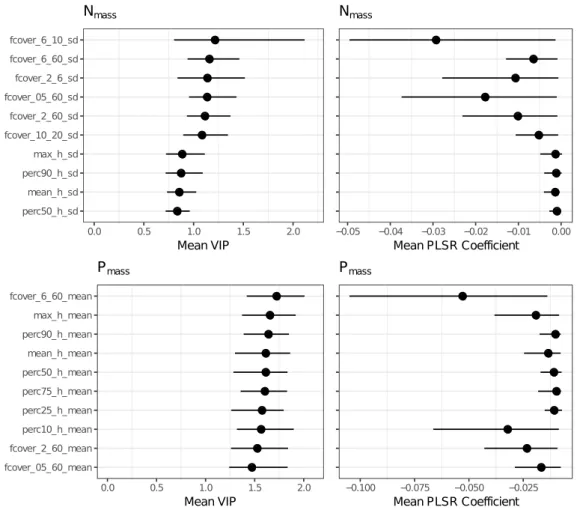
Table 2.1 Variables calculated from LiDAR point clouds in 3 m×3 m resolution. For the use in partial least squares regression models, variables were aggregated into a grid with a cell size of 24 m×24 m, by calculating mean and standard deviation.

LiDAR Metric Abbreviation Description

Minimum min_h_mean; min_h_sd Basic statistics Maximum max_h_mean; max_h_sd based on the Mean mean_h_mean; mean_h_sd height values of Standard deviation sd_h_mean; sd_h_sd vegetation LiDAR

Variance var_h_mean; var_h_sd points

Coefficient of variation cov_h_mean; cov_h_sd 10th percentile perc10_h_mean; perc10_h_sd 25th percentile perc25_h_mean; perc25_h_sd 50th percentile perc50_h_mean; perc50_h_sd 75th percentile perc75_h_mean; perc75_h_sd 90th percentile perc90_h_mean; perc90_h_sd

Fractional cover 0.5m – 2m fcover_05_2_mean; fcover_05_2_sd Inverse penetration Fractional cover 0.5m – 60m fcover_05_60_mean; fcover_05_60_sd ratios representing Fractional cover 2m – 6m fcover_2_6_mean; fcover_2_6_sd an estimate for Fractional cover 2m – 60m fcover_2_60_mean; fcover_2_60_sd fractional cover of Fractional cover 6m – 10m fcover_6_10_mean; fcover_6_10_sd the vegetation Fractional cover 6m – 60m fcover_6_60_mean; fcover_6_60_sd within given height Fractional cover 10m – 20m fcover_10_20_mean; fcover_10_20_sd thresholds

Fractional cover 20m – 60m fcover_20_60_mean; fcover_20_60_sd

From both imaging spectroscopy and LiDAR raster layers, we extracted values from all pixels overlapping with the 50 field plots to be used as input to the statistical models. For each plot, we calculated the weighted mean values of 245 hyperspectral bands and 19 LiDAR-variables (Tab. 2.1) from the extracted cell values, using the percent overlap of each cell with the plot area as weight. Similarly, we calculated the weighted standard deviation for LiDAR-derived variables which represent a measure of spatial heterogeneity of these variables.

For prediction we aggregated the pixels of the imaging spectroscopy and LiDAR raster layers to a grid with a pixel size of 24 m ×24 m, calculating the mean and the standard deviation (for LiDAR-derived variables only) of all aggregated cells. This finally resulted in a dataset containing 245 spectral bands and 38 LiDAR-derived variables (mean and standard deviation).

2.1.2.4 Model calibration and validation

For both response variables, Nmassand Pmass, we built predictive models using the extracted values from the raster layers at plot locations as predictors. We calculated partial least squares regression (PLSR) models with a step-wise backward model selection procedure implemented in the R package autopls (R Core Team, 2016; Schmidtlein et al., 2012). The

number of latent variables was chosen based on the lowest root mean squared error (RMSE) in leave-one-out cross-validation. Before model calibration predictors were normalized, dividing each predictor variable by its standard deviation.

To test the benefit of LiDAR-derived data for the prediction of community weighted means of Nmass and Pmass at the canopy level we fit two sets of models for each response variable, one incorporating the hyperspectral bands only and a second one using a combination of hyperspectral bands and LiDAR-derived variables as predictors. To test the independent contribution of LiDAR data on the predictions, we additionally fit a third set of models for both N_mass and P_mass including only LiDAR-derived variables as predictors. N_mass values were natural log transformed prior to the model calculations.

The model calculations and predictions were embedded in a resampling procedure with 200 permutations, in order to reduce the bias in model predictions, yielding to a better comparison between the three sets of models. In each permutation, a subsample of 40 out of the 50 field plots was randomly drawn without replacement and used for model calibration and validation. Each model was used to generate a prediction map with a grid size of 24 m × 24 m, resulting in 200 prediction maps for each response variable and each of the three predictor combinations used, respectively. From these maps we calculated a median prediction map and the associated coefficient of variation (CV), representing the spatial uncertainty of model predictions (Singh et al., 2015).

For the assessment of the predictive performance of the models, we calculated the mean Pearson r-squared as well as the absolute and normalized root mean squared error (RMSE) between predicted and observed values of each data subset. The same performance measures were calculated for each data subset in leave-one-out cross-validation data. For N_mass, r-squared values and RMSE were calculated based on the log-transformed dataset. The normalized RMSE was calculated by dividing the RMSE by the mean value in the response dataset. r-squared and RMSE values were used to compare the performances of models using only hyperspectral bands or a combination of hyperspectral bands and LiDAR-derived variables as predictors, for N_mass and P_mass respectively. Model performance is affected by the number of variables included, in the case of a PLSR the number of latent variables. To check for such an effect we grouped the corresponding models according to the number of latent variables included and compared the r-squared values for each group separately (supplementary material, Fig. 2.12).

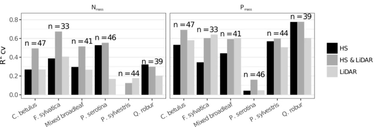
2.1.3 Results

Field plots were located in forest stands with heights ranging from 3 to 40 m and LAI values ranging from 1.7 to 5.9 (supplementary material, Tab. 2.4). Plot-wise community weighted mean values for N_mass and P_mass ranged from 13.8 to 25.4 g·kg−1 and from 0.82 to 1.93 g·kg−1, respectively. Nmass of P. serotina and P. sylvestris were significantly different from all other species (supplementary material, Fig. 2.13 and, Tab. 2.5). Contrary, we

observed no differences in measured N_mass between. F. sylvatica,Q. robur andC. betulus. Pmass differed significantly between all species except between C. betulus and Q. robur (supplementary material, Fig. 2.13). Models combining structural vegetation attributes,

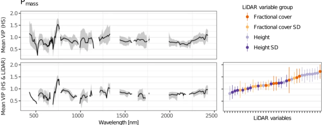
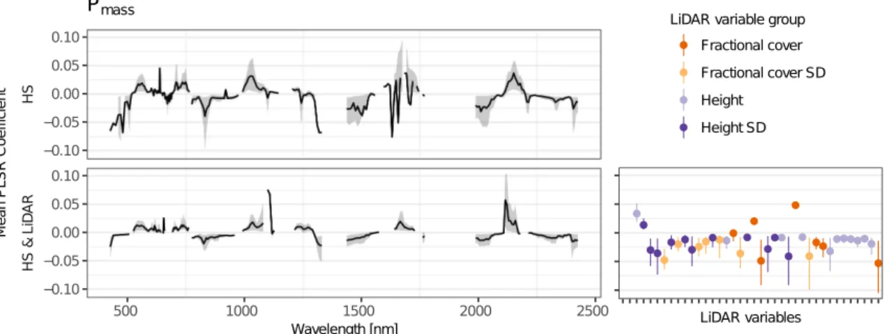
derived from airborne LiDAR, with imaging spectroscopy improved predictions of community weighted mean values for Nmass and Pmass compared to models using imaging spectroscopy data solely (Tab. 2.2, Fig. 2.2). In the combined Nmass models, hyperspectral bands had a significantly higher contribution (p < 0.001) to the variance explained, compared to LiDAR-derived variables (Fig. 1). By contrast, in Pmass models, LiDAR-derived variables showed a significantly higher contribution (p < 0.001). With respect to the selected spectral bands we observed only marginal differences between models including LiDAR-derived variables and models not including them (Figs. 2.3, 2.4, 2.5, 2.6).

Table 2.2 Results of PLSR models for Nmassand Pmassfrom 200 bootstraps. Predictors: used predictor

variables being either, hyperspectral bands (HS) or LiDAR-derived variables; # LV: mean number of latent variables; # Var: mean number of selected predictor variables;Rcal2 : mean coefficient of determination in

calibration;R2

cv: mean coefficient of determination in validation;RM SEcal: average root mean squared

error in calibration;RM SEcv: average root mean squared error in leave-one-out cross-validation

Response Predictors #LV #Var Rcal2 R

2

cvRMSEcalRMSEcv RMSEcalRMSEcv

[%] [%] Nmass∗ HS 5.8 98 0.47 0.31 0.09 0.09 2.9 3.3 ±0.10±0.14 ±0.01 ±0.01 HS & LiDAR 5.7 43 0.55 0.41 0.08 0.09 2.7 3.0 ±0.12±0.16 ±0.01 ±0.01 LiDAR 3.5 8 0.39 0.26 0.09 0.10 3.1 3.4 ±0.08±0.09 ±0.01 ±0.01 Pmass HS 6.3 42 0.59 0.45 0.15 0.18 13.1 15.3 ±0.15±0.16 ±0.02 ±0.02 HS & LiDAR 6.9 38 0.73 0.63 0.13 0.14 10.8 12.5 ±0.08±0.10 ±0.02 ±0.02 LiDAR 3.7 9 0.62 0.54 0.15 0.17 12.6 14.0 ±0.08±0.10 ±0.01 ±0.01 ∗natural log-transformed 0.00 0.25 0.50 0.75 1.00 HS LiDAR V IP p ro po rt io n

N

P

Figure 2.1 Relative contribution of hyperspectral bands (HS) and LiDAR variables to the variance explained in PLSR models for Nmass and Pmass expressed as proportion of the total VIP (Variable