Generalized Stacked Sequential
Learning
Eloi Puertas i Prats
Aquesta tesi doctoral està subjecta a la llicència Reconeixement- NoComercial – SenseObraDerivada 3.0. Espanya de Creative Commons.
Esta tesis doctoral está sujeta a la licencia Reconocimiento - NoComercial – SinObraDerivada 3.0. España de Creative Commons.
This doctoral thesis is licensed under theCreative Commons Attribution-NonCommercial-NoDerivs 3.0. Spain License.
Learning
Eloi Puertas i Prats
Department of Applied Mathematics and Analysis Universitat de Barcelona
Doctoral advisors: Dr. Oriol Pujol i Vila Dr. Sergio Escalera Guerrero
A thesis submitted in the Mathematics and Computer Science Doctorate Program
Doctor in Mathematics - Computer Science (PhD)
In many supervised learning problems, it is assumed that data is indepen-dent and iindepen-dentically distributed. This assumption does not hold true in many real cases, where a neighboring pair of examples and their labels ex-hibit some kind of relationship. Sequential learning algorithms take benefit of these relationships in order to improve generalization. In the literature, there are different approaches that try to capture and exploit this correla-tion by means of different methodologies. In this thesis we focus on meta-learning strategies and, in particular, the stacked sequential meta-learning (SSL) framework.
The main contribution of this thesis is to generalize the SSL highlighting the key role of how to model the neighborhood interactions. We propose an effective and efficient way of capturing and exploiting sequential correlations that take into account long-range interactions. We tested our method on several tasks: text line classification, image pixel classification, multi-class classification problems and human pose segmentation. Results on these tasks clearly show that our approach outperforms the standard stacked sequential learning as well as off-the-shelf graphical models such conditional random fields.
All men by nature desire to know. An indication of this is the delight we take in our senses; for even apart from their usefulness they are loved for themselves; and above all others the sense of sight. For not only with a view to action, but even when we are not going to do anything, we prefer
sight to almost everything else. The reason is that this, most of all the senses, makes us know and brings to light many differences between things.
First of all, I would like to thank my advisors Dr. Oriol Pujol and Dr Sergio Escalera for all the support they have giving me during all these years. Without your help this would not happen. Thank you both for your patience and everything else.
I would like to express my gratitude to all my colleagues of University of Barcelona, specifically those of the Department of Matem`atica Aplicada i An`alisi, thanks to them, work and lunch is always a pleasure.
Thanks to my parents Miquel i Rosa, brother Santi and sister Susana for having always been there for me.
Many thanks to David Masip, Carles Noguera, Jordi Campos, F`elix Bou, Santi Onta˜non for all the discussions we had and for the time we spent together. Guys, you really are an inspiration to me.
I would like to mention the members of IIIA-CSIC and Computer Vision Center research centers I had work with, who have shared with me their knowledge and expertise.
I would also like to take this opportunity to thank my lifelong mentors: Josep Maria Fortuny, Eva Armengol, Maria Vanrell, Philippe R. Richard, Markus Hohenwarter, Jordi Vitri`a, Francesc Esteve, Ramon L´opez de M´antaras and Carles Sierra. Special thanks goes to Nate Davison for your lessons of life, guitar and english!
Finally, last but not least, I would like to thank all my doctoral fellows in MAIA department: Ari Farr´es, Marta Canadell, Dani P´erez, David Mart´ı, Jordi Canela, Carlos Domingo, Ruben Berenguel, Narc´ıs, Marc, Roc, Giulia, Arturo, Nadia, Meri, Maya, Estefania, Miguel ´Angel, Toni, Miguel Reyes, Dani, Albert Clap´es, Cristina, Carles Riera, `Alex, Adriana, Santi, Laura,
twice!
Per acabar els agra¨ıments, ho far´e en la meva llengua mare, el catal`a. Cada mat´ı quan entro a l’edifici hist`oric de la Universitat de Barcelona, no puc deixar de pensar per un moment que per all`a mateix el meu avi Jaume, el meu avi Miguel, que nom´es he conegut en fotografies, i les meves `avies Joana i Adoraci´on deurien passejar-s’hi tot sovint. No puc, doncs, deixar de sentir orgull per tots els meus avis i els meus pares, per haver lluitat, sofert i finalment sortir-se’n endavant durant uns anys tant dif´ıcils com els que van haver de viure. El que he pogut gaudir durant tots aquests anys d’estudi, recerca i treball ´es gr`acies a la seva const`ancia i dedicaci´o.
Tamb´e vull aprofitar l’ocasi´o per agrair a tota la gent que des del moment en que vaig decidir comen¸car a fer un llarg cam´ı en l’Acad`emia han estat, en algun moment o un altre al meu costat. Els amics de deb´o sempre seran els millors aliats en els moments d’alegria i el millor refugi en els moments tristos.
Amb el Ferran, l’ `Alex, en Jony, la Ver`onica, el Guillem i el David hem apr`es a viure la Universitat. Amb l’Esteve i la Rosa, el David i l’ `Oscar hem passat els millors i pitjors moments. Amb el Carles, la Laia, la Su, l’ `Oscar, el N`estor, la Marta, el Paco, el Santi, el Jordi i la Camp hem passat els moments m´es heavys. Amb la Cemre, l’ `Angela i l’Amanda hem passat moments de tots colors, des dels m´es divertits al m´es surrealistes. Amb l’Ivette, l’Anna Bonfill, l’Elisabeth i l’Ariadna Valls, la N´uria i el Loki i la Carolina hem constatat que com el Vall`es no hi ha res. Amb el Jordi, l’Albert, l’Alfons hem descobert Catalunya des de Salses a Guardamar i de
fet del futbol m´es que un esport. Amb la Diamar i l’Albert, el Reixaquet i l’Alba i l’Helena, el Sergi i el Quim hem pogut comprovar que qualsevol nit pot sortir el sol i que casa seva ´es casa nostra, si ´es que hi ha cases d’alg´u. Amb la Sara hem rigut molt. Amb la Marta Palac´ın hem tingut llargues tert´ulies de caf´e sobre la Fe dels Set i la difer`encia entre plet`oric i plat`onic. Gr`acies a l’Anna Bertran per haver-me donat suport en iniciar aquest llarg cam´ı. Gr`acies a l’Anna Lliberia per aguantar-me quan no veia la llum al final del t´unel. I sobretot gr`acies a la Claire per haver-me acompanyat en aquest ´ultim tram.
Finalment agrair tamb´e a tots els estudiants d’Enginyeria Inform`atica de la Universitat de Barcelona que he tingut tots aquests anys i que m’han aguan-tat el rollo i suporaguan-tat les bronques. Especialment a l’Albert Rosado, Adrian Hermoso, David Trigo, Carles Riera, Albert Clap´es, `Alex Pardo, Matilde Gallardo, Albert Hu´elamo, Pablo Mart´ınez i Xavi Moreno; us asseguro que he apr´es m´es jo de vosaltres que no pas al rev´es.
Gr`acies a tots per ser com sou!
List of Figures ix
List of Tables xiii
1 Introduction 1 1.1 Overview of Contributions . . . 2 1.2 Outline . . . 4 1.3 List of publications . . . 4 2 Background 7 2.1 Sequential Learning . . . 7
2.1.1 Meta-Learning sequential learning . . . 8
2.1.1.1 Sliding and recurrent sliding window . . . 9
2.1.1.2 Stacked sequential learning . . . 10
2.1.2 Hidden Markov Models . . . 10
2.1.3 Discriminative Probabilisitic Graphical Models . . . 12
2.1.3.1 Maximum Entropy Markov model (MEMM) . . . 13
2.1.3.2 Conditional Random Fields (CRF) . . . 14
2.2 Contextual information in image classification tasks . . . 16
2.3 Sequential learning in multi-class problems . . . 17
2.4 Conclusions . . . 17
3 Generalized Stacked Sequential Learning 19 3.1 Generalized Stacked Sequential Learning . . . 20
3.2 Multi-Scale Stacked Sequential Learning (MSSL) . . . 21
3.2.1.1 Multi-resolution Decomposition . . . 22
3.2.1.2 Pyramidal Decomposition . . . 23
3.2.1.3 Pros and cons of multi-resolution and pyramidal decom-positions . . . 23
3.2.2 Sampling pattern . . . 24
3.2.3 The coverage-resolution trade-off . . . 26
3.3 Experiments and Results . . . 27
3.3.1 Categorization of FAQ documents . . . 27
3.3.2 Weizmann horse database . . . 31
3.3.2.1 Results on the resized Weizmann horse database . . . . 33
3.3.2.2 Results on the full size Weizmann horse database . . . 36
3.4 Results Discussion . . . 38
3.4.1 Blocking effect using the pyramidal decomposition . . . 42
3.5 Conclusions . . . 43
4 Extensions to MSSL 45 4.1 Extending the basic model: using likelihoods . . . 45
4.2 Learning objects at multiple scales . . . 46
4.3 MMSSL: Multi-class Multi-scale Stacked Sequential Learning . . . 48
4.3.1 Extending the base classifiers . . . 50
4.3.2 Extending the neighborhood functionJ . . . 51
4.4 Extended data set grouping: a compression approach . . . 52
4.5 Experiments and Results . . . 54
4.5.1 Horse image classification using shifting . . . 54
4.5.2 Flowers classification using shifting . . . 55
4.5.3 MSSL for multi-class classification problems . . . 57
4.5.3.1 Experimental Settings . . . 57
4.5.3.2 Numerical Results . . . 60
4.5.3.3 Qualitative Results . . . 63
4.5.3.4 Comparing among proposed multi-class MSSL techniques 70 4.6 Conclusions . . . 73
5 Application of MSSL for human body segmentation 75
5.1 Stage One: Body Parts Soft Detection . . . 76
5.2 Stage Two: Fusing Limb Likelihood Maps Using MSSL . . . 79
5.3 Experimental Results . . . 81
5.3.1 Dataset . . . 81
5.3.2 Methods . . . 82
5.3.3 Settings and validation protocol . . . 82
5.3.4 Quantitative Results . . . 83
5.3.5 Qualitative Results . . . 83
5.4 Conclusions . . . 84
6 Conclusions 87
2.1 Stacked sequential learning algorithm. . . 11
2.2 Graphical structures of HMM, MEMM and CRF for sequencial learning. 13 3.1 Block diagram for SSL . . . 20
3.2 Block diagram for GSSL . . . 20
3.3 Design ofJ(y′, ρ, θ) in MSSL . . . 21
3.4 Two examples of multi-scale decomposition . . . 22
3.5 A graphical representation of the displacements setρ . . . 25
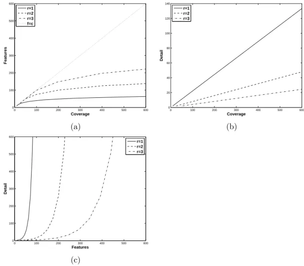
3.6 (a) number of features needed for covering a certain number of predicted values for different window sizesr, (b) detail with respect to the coverage, (c) number of features needed to consider a certain detail value . . . 26
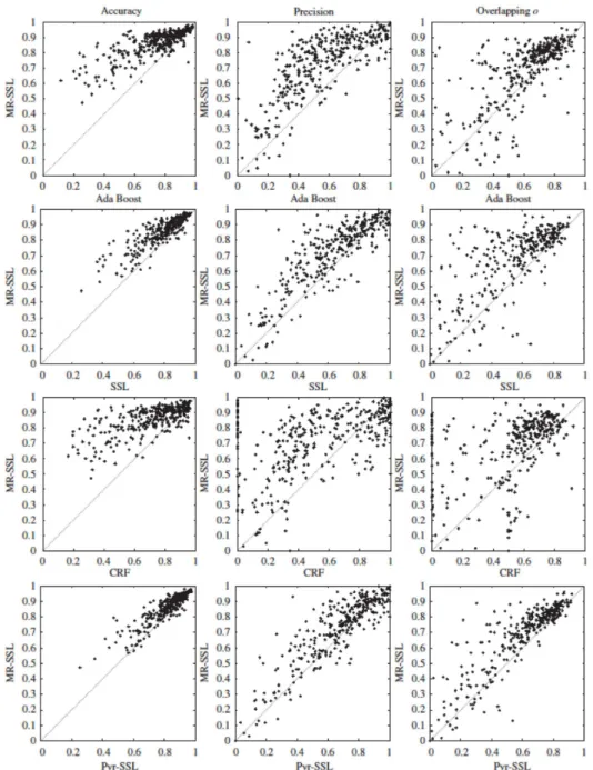
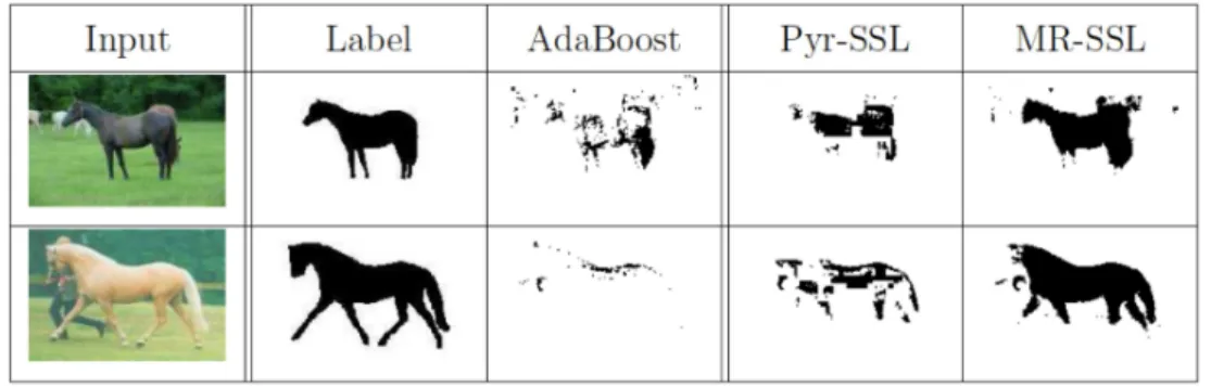
3.7 Comparison of the proposed MR-SSL method to AdaBoost (first row), SSL using a window of size 7×7 (second row), CRF (third row) and Pyr-SSL (last row) on the resized Weizmann horse database. . . 34
3.8 The best 30 segmentations on full size images. First column shows the input image, second column shows the ground truth, third column shows the classification result and the last column shows a color coded image with true positives (blue), true negatives (white), false positives (cyan) and false negatives (red). . . 37
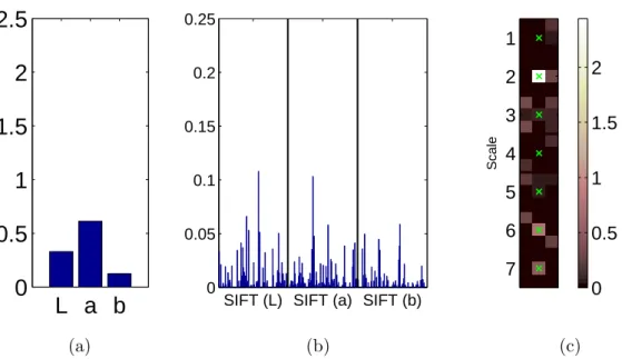
3.9 The weights Adaboost assigned to the (a) pixel-wise color features, (b) textural SIFT descriptor and (c) contextual features. The total weight of the pixel-wise color feature is 1.06 (10.2%), the total weight of SIFT features is 2.4 (23.2%) and the total weight of contextual features is 6.89 (66.6%). . . 39
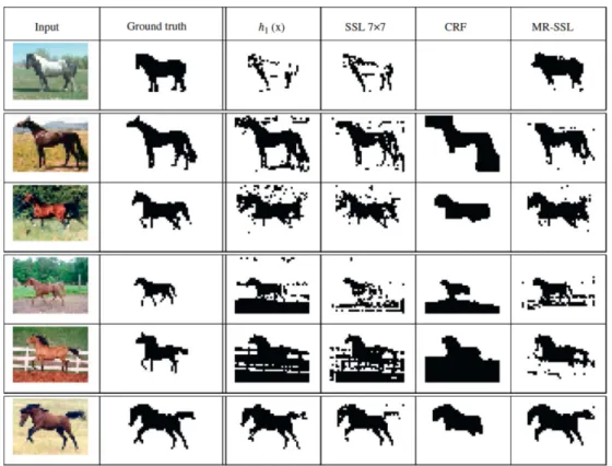
3.10 Input, ground truth and results of different methods on the test image
number 142. . . 39
3.11 Input, ground truth and results of different methods on the test image numbers: 84, 22, 71, 88, 108 and 109 respectively. . . 40
3.12 Label field multi-resolution decomposition classifying image number 84. 41 3.13 Input, ground truth and results of different methods on the test image number 41. . . 42
3.14 Input, ground truth and results of different methods on the test image number 153. . . 42
3.15 Visual comparison of the Pyr-SSL and the MR-SSL on images number 68 and 144. . . 43
4.1 Architecture of theshifting technique. . . 47
4.2 ECOCone-versus-one coding matrix. . . 49
4.3 Multi-class multi-scale stacked sequential learning . . . 50
4.4 5-class likelihood maps compressed to three, using partitions. Binary approach is represented by Table 1. The symbols used are 0 and 1. Ternary approach is represented by Table 2. The symbols used are -1 and 1. Applying Equation. 4.6we obtain the aggregated likelihood maps P1, P2, P3 ∈P. In the case of binary compression, any class marked with zero in a codeword Γ is not considered, while in the case of ternary com-pression, all classes are aggregated according to each of the codewords Γ. . . 53
4.5 Examples of horse classification. Second column shows Adaboost prediction. Third and forth uses MSSL over the images with and without shifting. . . 54
4.6 Predictions using Adaboost and MSSL. . . 56
4.7 Comparison of all methods against each other with the Nemenyi test. Groups of classifiers that are not significantly different are connected. . 64
4.8 Figures of final classification in motion sequential scenario and motion random scenario for ADAboost, multi-label optimization Graph cut, and our proposal MMSSL. Y-axe shows the labels for each class and X-axe is the time interval. Predictions values are marked with + and real values are marked just below with dots. . . 66
4.9 Figures of final classification in ETRIMS 4 Classes HOG database. (a) Shows the original image, (b) the groundtruth image, and (c),(d), and (e) show ADAboost, GraphCut, and MMSSL without compression, re-spectively. . . 67 4.10 Figures of final classification in ETRIMS 8 Classes HOG database. (a)
Shows the original image, (b) the groundtruth image, and (c),(d), and (e) show ADAboost, GraphCut, and MMSSL without compression, re-spectively. . . 68 4.11 Figures of final classification in IVUS using 6 scales. (a) Shows the
original image, (b) the groundtruth image, and (c),(d), and (e) show ADAboost, GraphCut, and MMSSL without compression, respectively. . 69 4.12 Comparative between multi-class multi-scale stacked sequential learning
approaches in ETRIMS 4 Classes HOG database. (a) Shows the original image, (b) the groundtruth image, and (c), (d), (e), and (f) shows the different MMSSL schemes: (c) MMSSL using only label predictions, (d) MMSSL using confidences, (e) MMSSL using binary compression, and (f) MMSSL using ternary compression . . . 71 4.13 Comparative between multi-class multi-scale stacked sequential learning
approaches in ETRIMS 8 Classes HOG database. (a) Shows the original image, (b) the groundtruth image, and (c), (d), (e), and (f) shows the different MMSSL schemes: (c) MMSSL using only label predictions, (d) MMSSL using confidences, (e) MMSSL using binary compression, and (f) MMSSL using ternary compression. . . 72
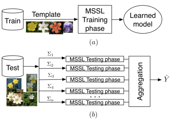
5.1 Method overview. (a) Abstract pipeline of the proposed MSSL method where the outputsY′
i of the first multi-class classifierH1(x) are fed to the multi-scale decomponsition and sampling functionJ(x) and then used to train the second stacked classifierH2(x) which provides a binary output ˆY. (b) Detailed pipeline for the MSSL approach used in the human segmentation context whereH1(x) is a multi-class classifier that takes a vector X of images from a dataset. As a result, a set of likelihood maps Y′
1. . . Yn′ for each part is produced. Then
a multi-scale decomposition with a neighborhood sampling function J(x) is applied. The output X′ produced is taken as the input of the second classifier
H2(x), which produces the final likelihood map ˆY, showing for each point the confidence of belonging to human body class. . . 78 5.2 (a) Tree-structure classifier of body parts, where nodes represent the defined
dichotomies. Notice that the single or double lines indicate the meta-class defined. (b) ECOC decoding step, in which a head sample is classified. The coding matrix codifies the tree-structure of (a), where black and white positions are codified as +1 and−1, respectively. c,d,y,w,X, andδcorrespond to a class category, a dichotomy, a class codeword, a dichotomy weight, a test codeword, and a decoding function, respectively. . . 79 5.3 Limb-like probability maps for the set of 6 limbs and body-like probability map.
Image (a) shows the original RGB image. Images from (b) to (g) illustrate the limb-like probability maps and (h) shows the union of these maps. . . 80 5.4 Comparative betweenH1andH2output. First column are the original images.
Second column are H2 output likelihood maps. Last column are the union of all likelihood map of body parts . . . 81 5.5 Different samples of the HuPBA 8k+ dataset. . . 82 5.6 Samples of the segmentation results obtained by the compared approaches. . . 86
3.1 Average percentage error and methods ranking for different FAQ data-sets, different methods; and different parameterization of SSL, Pyr-SSL and MR-SSL. For the sake of table compactness, the following definitions should be considered: ρ3 = {−3,−2, . . . ,2,3}, ρ6 = {−6,−5, . . . ,5,6},
ρ1={−1,0,1}. . . 29
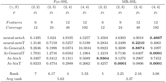
3.2 Average percentage error for different configurations of Pyr-SSL and MR-SSL. The last two rows show the average rank for each parameterization as well as the average rank for each of the multi-scale families. . . 30 3.3 The average performance of AdaBoost, SSL (7×7 window size),
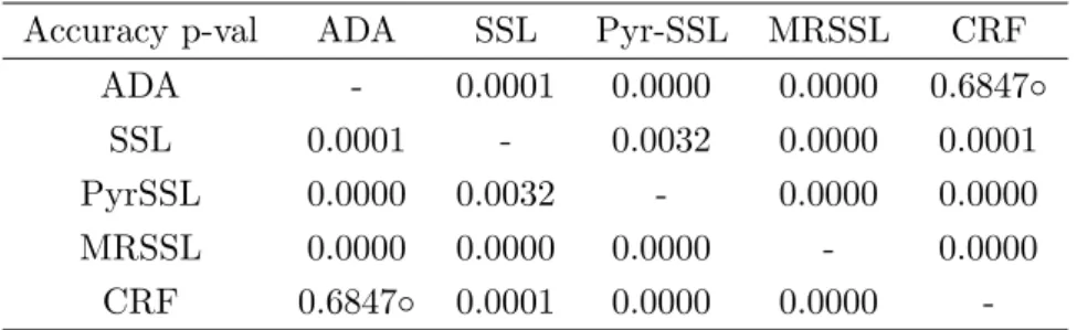
MR-SSL, CRF and Pyr-SSL in terms of Accuracy, Precision and Overlapping. Standard deviations are in brackets. . . 33 3.4 Wilcoxon paired signed rank test p-values for the results of the accuracy
measure. . . 35 3.5 Wilcoxon paired signed rank test p-values for the results of the
overlap-ping measure. . . 35 3.6 The average performance of AdaBoost and MR-SSL in terms of
Accu-racy, Precision and Overlapping; adding 27 Haar-like features to the first feature vector x. Standard deviations are in brackets. . . 36 3.7 The average performance of AdaBoost and MR-SSL in terms of
Accu-racy, Precision and Overlapping using the color plus SIFT descriptor as the first feature vector x. Standard deviations are in brackets. . . 38 4.1 Results of prediction using Adaboost and MSSL with and without shifting
technique. . . 55 4.2 Results using Adaboost and MSSL. . . 56
4.3 Result figures for database motion sequential scenario. . . 60
4.4 Result figures for database motion random scenario. . . 60
4.5 Result figures for database motion one person. . . 61
4.6 Result figures for database FAQ. . . 61
4.7 Result figures for database IVUS, using 6 scales. . . 61
4.8 Result figures for database ETRIMS 4 classes RGB and HOG. . . 62
4.9 Result figures for database ETRIMS 8 classes RGB and HOG. . . 62
4.10 Mean rank of each strategy considering the accuracy terms of the differ-ent experimdiffer-ents. . . 63
5.1 Overlapping results over the 9 folds of theHupBA8K+dataset for the proposed MSSL method and the Soft detectors post-processing their outputs with the Graph-Cuts method and GMM Graph-Cuts method. . . 84
Input data
X Set of input samples
x An input sample
Ci Theith class out of a total ofN
y∈ {C1, C2, . . . , CN} Ground truth labels Multi-scale SSL
H1(x), H2(x) Two classifiers working on the i.i.d. hypothesis
y′ Predicted label value byh1(x)
ˆ
Y Final MSSL prediction produced byh2(x
ext
) ˆ
F(x,c) A prediction confidence map
J(y′, ρ, θ) A functional that models the labels context
θ Neighborhood parameterization
ρ Set of displacement vectors
M Cardinality ofρ
~
ρm∈ρ A generic displacement vector z∈Rw
The contextual feature vector produced byJ w∈N The length of the contextual feature vectorz
xext
The extended feature vector combining xandz
Σ Set of scales
s∈ {1,2, . . . , S} Index of the Σ scales
G(µ, σ) Multi-dimensional Gaussian distribution Φ(s) Multi-resolution decomposition
Ψ(s) Pyramidal decomposition
Multiclass MSSL
n Number of dichotomizers
b A dichotomizer
M ECOC coding matrix
Y A class codeword in ECOC framework
X A sample prediction codeword in ECOC framework
mx Margin for a prediction of samplex
β Constant which governs transition in a sigmoidean function
δ A soft distance
α Normalization parameter for soft distanceδ
P A set of partitions of classes
P A partition of groups of classes
γ A symbol in a partition codeword Γ A partition codeword
Experiments settings
R The mean ranking for each system configurations
E The total number of experiments
k The total number of system configuration
χ2
F Friedman statistic value
Introduction
Over the past few decades, machine learning (ML) algorithms have become a very useful tool in tasks where designing and programming explicit, rule-based algorithms are infeasible. Some examples of applications where machine learning has been applied successfully are spam filtering, optical character recognition (OCR), search engines and computer vision. One of the most common tasks in ML is supervised learning, where the goal is to learn a general model able to predict the correct label of unseen examples from a set of known labeled input data. In supervised learning often it is assumed that data is independent and identically distributed (i.i.d). This means that each sample in the data set has the same probability distribution as the others and all are mutually independent. However, classification problems in real world databases can break this i.i.d. assumption. For example, consider the case of object recognition in image understanding. In this case, if one pixel belongs to a certain object category, it is very likely that neighboring pixels also belong to the same object, with the exception of the borders. Another example is the case of a laughter detection application from voice records. A laugh has a clear pattern alternating voice and non-voice segments. Thus, discriminant information comes from the alternating pattern, and not just by the samples on their own. Another example can be found in the case of signature section recognition in an e-mail. In this case, the signature is usually found at the end of the mail, thus important discriminant information is found in the context. Another case is part-of-speech tagging in which each example describes a word that is categorized as noun, verb, adjective, etc. In this case it is very unlikely that patterns such as [verb, verb, adjective, verb] occur. All these applications present a common feature: the sequence/context of the labels matters.
not independently drawn from a joint distribution of the data samples X and their labelsY. In sequential learning the training data actually consists of sequences of pairs (x, y), so that neighboring examples exhibit some kind of correlation. Usually sequential learning applications consider one-dimensional relationship support, but these types of relationships appear very frequently in other domains, such as images, or video.
Sequential learning should not be confused with time series prediction. The main difference between both problems lays in the fact that sequential learning has access to the whole data set before any prediction is made and the full set of labels is to be provided at the same time. On the other hand, time series prediction has access to real labels up to the current time t and the goal is to predict the label at t+ 1. Another related but different problem is sequence classification. In this case, the problem is to predict a single label for an input sequence. If we consider the image domain, the sequential learning goal is to classify the pixels of the image taking into account their context, while sequence classification is equivalent to classify one full image as one class. Sequential learning has been addressed from different perspectives: from the point of view of meta-learning by means of sliding window techniques, recurrent sliding windows or stacked sequential learning where the method is formulated as a combination of classifiers; or from the point of view of graphical models, using for example Hidden Markov Models or Conditional Random Fields.
In this thesis, we are concerned with meta-learning strategies. Cohen et al. (17) showed that stacked sequential learning (SSL from now on) performed better than CRF and HMM on a subset of problems called “sequential partitioning problems”. These problems are characterized by long runs of identical labels. Moreover, SSL is computationally very efficient since it only needs to train two classifiers a constant number of times. Considering these benefits, we decided to explore in depth sequential learning using SSL and generalize the Cohen architecture to deal with a wider variety of problems.
1.1
Overview of Contributions
The contributions of this thesis aim to give solutions to the open problems in sequential learning described in (25) which are: a) how to capture and exploits sequential corre-lations; b) how to represent and incorporate complex loss functions; c) how to identify long-distance interactions; d) how to make sequential learning computationally efficient. Our first contribution is a generalization of the SSL framework. We argue that a fundamental and overlooked step in SSL is the way in which the extended set (which
is fed into the second classifier) is created. Instead of creating the extended set using a standard window approach, we propose a new aggregation method capable of capturing long-distance interactions efficiently. This method (MSSL) is based on a multi-scale decomposition of the first classifier predictions. In this way, we provide answers to the above open questions obtaining a method that: a) captures and exploit sequential correlations; b) since the method is a meta-learning strategy the loss function depen-dency is delegated to the second step classifier; c) it efficiently captures long-distance interactions; and d) it is fast, because it relies on training a few general learners.
Starting from this general framework, we propose a range of extensions with the purpose of making our architecture usable in a broader number of applications. By using theses extensions, our framework provides a general way for the classification of objects at different scales as well as for performing multi-class classification in an efficient way.
Our concluding contribution is an application of our framework for human body segmentation.
Summarizing, the main contributions of this thesis are:
• Multiscale Stacked Sequential Learning: A generalization of the SSL framework where the extended set is built by applying a multi-scale decomposition of the first classifier predictions.
• Scale invariant MSSL: An extended architecture of the MSSL framework useful when objects appear at different scales. Using this methodology different sized objects can be classified correctly without retraining.
• Multi-class MSSL: A way to extend MSSL to multi-class classification problems. By applying the ECOC framework in the base classifiers of MSSL and converting predictions to a likelihood measure we propose a general way to use MSSL in multi-class classification
• Memory-efficient multi-class MSSL: A compression approach of multi-class MSSL for reducing the number of features in the extended set depending on the number of classes.
• Application of MSSL for human body segmentation: An application of MSSL framework for human body segmentation. Here results show that our framework gives useful contextual information about joint body parts, helping to improve final classification accuracy.
1.2
Outline
This thesis proceeds as follows:
Chapter 2: Background. Chapter2covers some background material on sequential learning from several points of view inside machine learning: meta-learning, hid-den markov models and discriminative probabilistic graphical models. Moreover, from the side of computer vision, works related to contextual information are also described. Finally some works specifically related to sequential learning applied to multi-class problems are shown.
Chapter 3: Generalized Stacked Sequential Learning. In chapter 3 we intro-duce our main contribution to the sequential learning problem. First a gener-alization of the called stacked sequential learning method is described. Next, an implementation of the proposed multi-scale stacked sequential learning (MSSL) method is presented explained. Finally, experiments and results comparing our methodology with other sequential learning approaches are discussed.
Chapter 4: Extensions to MSSL. Chapter 4 provides several improvements over MSSL framework. First the inclusion of likelihoods measures instead of class la-bels in the stacked pipeline is proposed. Next, we show the extended architecture of our framework, where objects can be classified at different scales without re-training. In addition, a general methodology for multi-class classification problem is integrated with MSSL framework. Finally, an approach for compressing the number of features in the stacked pipeline is described.
Chapter 5: Application of MSSL for human body segmentation. In chapter5 an application of MSSL for human body segmentation is described. Here the stacked pipeline is modified to be used along with cutting-edge technologies for body segmentation.
Chapter 6: Conclusions. Chapter6concludes this thesis, highlighting the most rel-evant contributions of this work.
1.3
List of publications
Much of the work presented here has appeared first in other publications. The results of Chapter 3 appeared in (34), though the discussion here is extended. The extension to our MSSL framework learning objects at multiple scales described in Chapter 4
appeared in (52). The multi-class and the compression of the extended set appeared in (53).
Finally the application of MSSL for human body segmentation has been published in the ECCV14 workshopChaLearn Looking at People: pose recovery, action/interaction, gesture recognition that will be held in Zurich, Switzerland from September 6th to 12th 2014 (54).
In addition of these publications, preliminary results were presented in high relevant conferences in the area. A comprehensive list of all the contributions is found in the following lines:
• (2009) Multi-modal laughter recognition in video conversations. S Escalera, E Puertas, P Radeva, O Pujol. Computer Vision and Pattern Recognition Work-shops, 2009. CVPR Workshops. IEEE Computer Society Conference on,
• (2009) Multi-scale stacked sequential learning. O Pujol, E Puertas, C Gatta.
Multiple Classifier Systems, 262-27.
• (2009) Multi-Scale Multi-Resolution Stacked Sequential Learning. E Puertas, C Gatta, O Pujol. Proceedings of the 12th International Conference of the Catalan Association for Artificial Intelligence (CCIA). 112-117.
• (2010) Classifying Objects at Different Sizes with Multi-Scale Stacked Sequential Learning. E Puertas, S Escalera, O Pujol Proceedings of the 10th International Conference of the Catalan Association for Artificial Intelligence (CCIA), 193-200. • (2011) Multi-scale stacked sequential learning. C Gatta, E Puertas, O Pujol.
Pattern Recognition 44 (10), 2414-2426
• (2011) Multi-class multi-scale stacked sequential learning. E Puertas, S Escalera, O Pujol. Multiple Classifier Systems, 197-206
• (2013) Generalized multi-scale stacked sequential learning for multi-class classi-fication. E Puertas, S Escalera, O Pujol. Pattern Analysis and Applications, 1-15
Additionally, in the following lines a list of other coauthored published works related to this PhD is given:
• (2010) Adding Classes Online in Error Correcting Output Codes Framework. S Escalera, D Masip, E Puertas, P Radeva, O PujolICPR 2010, 2945-2948
• (2011) Online error correcting output codes. S Escalera, D Masip, E Puertas, P Radeva, O Pujol. Pattern Recognition Letters 32 (3), 458-467
Background
In this chapter we first explain the sequential learning concept. Next, previous works related to sequential learning from different points of view are described. Besides these related works coming from the machine learning field, sequential learning can be applied in computer vision problems as a tool for contextual information retrieval. Therefore, relevant works in this area are also commented. To conclude this chapter, we point out some works related to sequential learning but explicitly in the case of multi-class problems.
2.1
Sequential Learning
The classical supervised learning problem consists in constructign a classifier that can correctly predict the classes of new objects given training examples of already known objects (48). This task is typically formalized as follows:
Let assume the problem domain of classifying a pixel of an image to the class which it belongs to. LetXdenote an image of an object of interest andY ∈ {C1, C2, ..., CN}
denote the corresponding ground truth label image. A training example is a pair (x,y) consisting of a pixel of the image and its associated class label. We assume that the training examples are drawn independently and identically from the joint distribution P(x,y), and we will refer to a set ofnsuch examples as the training data. A classifier is a functionHthat maps from images to classes. The goal of the learning process is to find anHthat correctly predicts the classy=H(x) for each pixelxfrom a new image. This is accomplished by searching some space H of possible classifiers for a classifier that produces good results on the training data without overfitting. One thing that is apparent in this and other applications is that they do not quite fit the supervised
learning framework. Rather than being drawn independently and identically (i.i.d.) from some joint distributionP(x,y), the training data actually consist of sequences of (x,y) pairs. These sequences exhibit significant sequential correlation. That is, nearby x and y values are likely to be related to each other. Sequential patterns are important because they can be exploited to improve the prediction accuracy of our classifiers, as in the case of image segmentation, where surrounding pixels belong to the same class, except for the ones on the edges.
Sequential learning (25) breaks the independent and identically distributed (i.i.d.) assumption and assumes that samples are not independently drawn from a joint dis-tribution of the data samplesXand their labelsY. In sequential learning the training data consists of sequences of pairs (x,y), and the goal is to construct a classifier H that can correctly predict a new label sequenceY =h(X) given an input sequence X. Sequential learning is often confused with two other, closely-related tasks. The first of these is the time-series prediction problem. The main difference between both problems lays in the fact that sequential learning has access to the whole data set before any prediction is made and the full set of labels is to be provided at the same time. On the other hand, time series prediction has access to real labels up to the current time t and the goal is to predict the label att+ 1. The second closely-related task is sequence classification. In this task, the problem is to predict a single label y that applies to an entire input sequenceX. For example, in the case of images, instead of classifying each pixel of the image, simply to say whether the whole image belongs to a class or another.
In literature, sequential learning has been addressed from different perspectives. We split them into three big families: a) from the point of view of meta-learning techniques, b) from the point of view of hidden markov models and c) from the point of view of various probabilistic graphical models.
2.1.1 Meta-Learning sequential learning
Meta-learning techniques (71) use a combination of different classifiers in order to predict a test example. The idea is to extend the classical supervised learning problem in a recursive fashion, where each step is aimed to obtain better results than the previous, but without overfitting. Recurrent sliding windows and stacked learning are well-known meta-learning strategies. In next subsections they are explained whitin the context of sequential learning,
2.1.1.1 Sliding and recurrent sliding window
The sliding window method converts the sequential supervised learning problem into the classical supervised learning problem. It constructs a classifier H that maps an input window of width w into an single output value y. Specifically, let d = (w−1)/2 be the half-width of the window. Then H predicts yi using the window
[xt−d, xt−d+1, . . . , xt, . . . , xt+d−1, xt+d]. The window classifier H is trained by
convert-ing each sequential trainconvert-ing example (xi,yi) into windows and then applying a standard
supervised learning algorithm. A new sequence x is classified by converting it to win-dows, applying H to predict each y to form the predicted sequence Y. The obvious advantage of this sliding window method is that it permits any classical supervised learning algorithm to be applied. Although the sliding window method gives adequate performance in many applications(29,55,63), it does not take advantage of correlations between nearby yt values. To be more precise, the only relationships between nearby yt values that are captured are those that are predictable from nearby xt values. If
there are correlations among the yt values that are independent of thext values, then
these are not captured. One way that sliding window methods can be improved is to make them recurrent. In a recurrent sliding window method, the predicted valueytis
fed as an input to help make the prediction for yt+1. Specifically, with a window of
half-widthd, the most recentdpredictions,yt−d, yt−d+ 1, . . . , yt−1, are used as inputs
(along with the sliding window [xt−d,xt−d+1, . . . ,xt, . . . ,xt+d−1,xt+d] ) to predictyt.
Clearly, the recurrent method captures predictive information that was not being cap-tured by the simple sliding window. The values used for theytinputs when training the
classifier can be achieved by means of meta-learning; by training a first non-recurrent classifier, and then use itsytpredictions as the inputs. This process can be iterated, so
that the predicted outputs from each iteration are employed as inputs in the next iter-ation. Another approach is to use the correct labelsytas the inputs. The advantage of
using the correct labels is that training can be performed with the standard supervised learning algorithms, since each training example can be constructed independently. On the other hand, when correct labels are used instead of predicted labels, the window classifier can overfit, thus the features used during the training will be much more ac-curate than the ones used during testing, leading the classifier to a higher testing error by relying on not trustworthy features. By using a first non-recurrent classifier we can know the a priory accuracy of the predictions features that will be used during the testing phase, resulting in a more reliable testing error.
2.1.1.2 Stacked sequential learning
Stacked sequential learning is a meta-learning (71) method, in which an arbitrary base learner is augmented, in this case, by making the learner aware of the labels of nearby examples. Basically, the stacked sequential learning (SSL) scheme is a two layers clas-sifier where, firstly, a base clasclas-sifier H1(x) is trained and tested with the original data
X. Then, an extended data set is created which joins the original training data features X with the predicted labels Y′ produced by the base classifier considering a fixed-size window around the example. Finally, a second classifierH2(x) is trained with this new
feature set. Then the inference algorithm takes part. Using the trained model of H1
on new instancesx, a set of predictions ˆy are obtained. With these predictions, a new extended set instancexext is constructed as above. Finally, using the trained model of
H2 on this extended set, a final set of predictions ˆY are obtained. Figure2.1describes
the SSL algorithm. The main drawback of the SSL approach is that the width of the window around the sample determines the maximum length of interaction among sam-ples. Therefore, the longer the window, the further the interaction is considered, but also the extended data set is increased in terms of features. This makes this approach not suitable for problems that present long range sequential relationships. Further-more, if we consider more than one relationship dimension, the size of the extended set increases exponentially, making it not feasible for sequential type of datasets like images.
2.1.2 Hidden Markov Models
The hidden Markov Model (HMM (1,56)) is a statistical Markov model in which the system being modeled is assumed to be a Markov process with unobserved (hidden) states. A HMM can be presented as the simplest dynamic Bayesian network. HMM describes the joint probability P(x,y) of a collection of hidden and observed discrete random variables. It is defined by two probability distributions: the transition distri-bution P(yt|yt−1), which tells how adjacent y values are related, and the observation
distributionP(x|y), which tells how the observed xvalues are related to the hidden y values. It relies on the assumption that thetth hidden variable given the (t−1)th
hid-den variable is indepenhid-dent of previous hidhid-den variables, and the current observation variables depend only on the current hidden state. These distributions are assumed to be stationary (i.e., the same for all times t). In most learning problems, x is a vector of features (x1, . . . , xn), which makes the observation distribution difficult to handle
Parameters: a neighborhood window of size W, a cross-validation parameter K, two base classifiers H1 and H2
Result: prediction ˆy=H2x
Learning algorithm: Given a data setX={(xt,yt)}
// Construct a sample of predictions Yt′ for each xt∈X as follows:
1. SplitX intoK equal-sized disjoint subsetsX1, . . . , Xk
for i←1toK do 2. fj ←H1(X−Xj)
end for
3. Y′ ← {(xt,y′t) :yt′ ← fj(xt);x∈Xj}
// Construct an extended setxext
4. xext← (x
t′,yt) :xt′ ←[x′1, . . . ,x′t] wherex′i←(xi, yi′−W, . . . , yi′+W) andyi′ is
thei-th component of y′t, the label vector paired withxt∈Y′
return {f ←H1(X),f′ ←H2(xext)}
Inference algorithm: Given an instance vector x 1. ˆy←f(x)
2. Construct an extended set instancexext, as above (using ˆy instead ofy′
t)
return Yˆ ←f′(xext)
independently (conditioned on y). This means that P(x|y) can be replaced by the product of n separate distributionsP(xj|y), j = 1, . . . , n.
In a sequential supervised learning problem, it is straightforward to determine the transition and observation distributions. P(yt|yt−1) can be computed by looking at
all pairs of adjacent y labels Similarly, P(xj|y) can be computed by looking at all
pairs of xj and y. The most complex computation is to predict a value ˆy given an
observed sequence x. Because the HMM is a representation of the joint probability distribution P(x,y), it can be applied to compute the probability of any particular y given any particular x : P(y|x). Hence, for an arbitrary loss function L(ˆy, y), the optimal prediction is:
ˆ y= arg min z X y P(y|x)L(z, y).
In the case where the loss function decomposes into separate decisions for eachyt, the
Forward-Backward algorithm (56) can be applied. Rather, where the loss function de-pends on the entire observed sequence, the goal is usually to find theywith the highest probability: y = arg maxyP(y|x). This can be solved by the dynamic programming algorithm known as the Viterbi algorithm (56), that computes, for each class label c and each time step t, the probability of the most likely path starting at time 0 end ending at timet with class u. When the algorithm reaches the end of the sequence, it has computed the most likely path from time 0 to timeti and its probability.
Although HMMs provide an elegant and sound methodology, they suffer from one principal drawback: any relationship relying on long-range interactions (this is, involv-ing not only two consecutiveyvalues) cannot be captured by a first-order Markov model (i.e., where P(yt) only depends on yt−1). A second problem with the HMM model is
that it generates eachxt only from the correspondingyt. This makes it difficult to use
an input window, moreover if the input window is not just of one dimension, but two, like in the case of images, where there exists a spatial relationship.
2.1.3 Discriminative Probabilisitic Graphical Models
Several directions have been explored to try to overcome the limitations of the HMM. The introduction of probabilistic graphical models that represent discriminative model P(y|x) rather than the generative modelP(x,y) is one of these directions. These mod-els do not try to explain how thex’s are generated. Instead, they just try to predict the yvalues given thex’s. In a generative model, one expends efforts to model the joint dis-tributionP(x,y), which involves implicit modeling of the observations x. This means that the generative approach may spend a lot of resources on modeling the generative
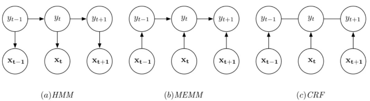
yt −1 yt yt+1 xt −1 xt xt+1 (a)HMM yt −1 yt yt+1 xt −1 xt xt+1 (b)MEMM yt −1 yt yt+1 xt −1 xt xt+1 (c)CRF
Figure 2.2: Graphical structures of HMM, MEMM and CRF for sequencial learning.
models which are not particularly relevant to the task of inferring the class labels. This permits them to use arbitrary features of the x’s including global features, features describing non-local interactions, and sliding windows. Moreover, discriminative ap-proaches can be particularly beneficial in cases where the domain of xis very large or even infinite. Some examples of discriminative graphical models are: Maximum En-tropy Markov models (MEMM (47)), Input-Output HMM (IOHMM (5)), Conditional random fields (CRF (44)). Figure2.2shows the graphical structures of HMM which is a purely generative model, MEMM which is a discriminative model, hence it represents a conditional distributionP(y|x) and CRF which is also discriminative model but here the interactions between the labelsy are modeled as undirected edges.
2.1.3.1 Maximum Entropy Markov model (MEMM)
A maximum-entropy Markov model (MEMM), or conditional Markov model (CMM), is a probabilistic graphical model that combines features of hidden Markov models (HMMs) and maximum entropy (MaxEnt) models. An MEMM is a discriminative model that extends a standard maximum entropy classifier by assuming that the un-known values to be learnt are connected in a Markov chain rather than being con-ditionally independent of each other, i.e. it learns P(yt|yt−1,xt). It is trained via a
maximum entropy method that attempts to maximize the conditional likelihood of the data: Qni=1P(yi|yi−1,xt). The maximum entropy approach represents P(yt|yt−1,xt)
as a log-linear model: P(yt|yt−1,x) = 1 Z(x, yt−1) exp X a λafa(x, yt) ! ,
where, thefa(x,yt) are real-valued or categorical feature-functions that can depend
onyt and on any properties of the input sequencex, andZ(x,yt−1) is a normalization
corre-sponds to the maximum entropy probability distribution satisfying the constraint that the empirical expectation for the feature is equal to the expectation given the model:
Ee[fa(x,y)] = Ep[fa(x,y)] ∀a.
The parameters λa can be estimated using generalized iterative scaling (21). The
optimal state sequencey1, . . . , yn can be found using a very similar Viterbi algorithm
to the one used for HMMs.
Bengio and Frasconi (5) introduced a variation of MEMM called Input-Output HMM (IOHMM). It is similar to the MEMM except that it introduces hidden state variablesst in addition to the output labelsyt. Sequential interactions are modeled by
the st variables. To handle these hidden variables during training, the
Expectation-Maximization (EM (22)) algorithm is applied.
One drawback of MEMMs and IOHMM models is that they potentially suffer from the ”label bias problem”. Notice that in MEMM model:
X yt P(yt|yt−1,x1, . . . ,xt) = X yt P(yt|yt−1,xt)·P(yt−1|x1, . . . ,xt−1) = 1·P(yt|yt−1,x1, . . . ,xt−1) =P(yt|yt−1,x1, . . . ,xt−1)
This says that the total probability mass “received” byyt−1 (based onx1, . . . , xt−1)
must be “transmitted” to labels yt at time t regardless of the value of xt. The only
role of xt is to influence which of the labels receive more of the probability at time t.
In particular, all of the probability mass must be passed on to some yt even if xt is
completely incompatible withyt. Thus, observations xt from later in the sequence has
absolutely no effect on the posterior probability of the current state; or, in other words, the model does not allow for any smoothing.
Conditional random fields (CRF) (44) were designed to overcome this weakness, which had already been recognized in the context of neural network-based Markov models in the early 1990s. Another source of label bias is that training is always done with respect to known previous predictions, so the model struggles at test time when there is uncertainty in the previous prediction.
2.1.3.2 Conditional Random Fields (CRF)
Conditional random fields (44) are a type of discriminative undirected probabilistic graphical model. In the CRF, the relationship among adjacent pairs yt−1 and yt is
words, the way in which the adjacent y values influence each other is determined by the input features. It is used to encode known relationships between examples and construct consistent interpretations. The CRF is represented by a set of potentials Mt(yt−1, yt|x), for each position in tin the sample sequence x, it is defined as:
Mt(yt−1, yt|x) = exp(Λt(yt−1, yt|x)) Λt(yt−1, yt|x) = X k λkfk(yt−1, yt,x) + X k µkgk(yt,x),
where thefkare features that encode some information aboutyt−1,yt, and arbitrary
information aboutx, and thegkare features that encode some information aboutytand
x. It is assumed that bothfk and gk are given and fixed. In this way, it is possible to
incorporate arbitrarily long-distance information aboutx. The conditional probability P(y|x) is written as: P(y|x) = Qn+1 t=1 Mt(yt−1, yt|x) hQn+1 t=1 Mt(x) i start,stop ,
where y0 = start and yn+1 = stop. The normalizer in the denominator is needed
because the potentialsMt are unnormalized ”scores”.
The training of CRFs is expensive, because it requires a global adjustment of the λ values. This global training is what allows the CRF to overcome the label bias problem by allowing thextvalues to modulate the relationships between adjacent yt−1
and yt values. Algorithms based on iterative scaling and gradient descent have been
developed for optimizing both P(y|x) and also for separately optimizing P(yt|x) for
loss functions that depend only on the individual label. Whereas in HMMs or MEEMs case, each gradient step required only a single execution of inference, when training a CRF, we must execute inference for every single data case, conditioning on variablesx. This makes the training phase considerably more expensive than HMMs or MEMMs. For example, in image classification task, inference step using a generative method involves summation over the space of all possible images; if we haveN×N image where each pixel can take 256 values, the resulting space has 256N2
values, giving rise to a highly intractable inference problem (even using approximate inference methods). The next section shows other methods and approaches that particularly exploit contextual information in image classification tasks.
2.2
Contextual information in image classification tasks
While the contribution of this thesis can appear limited into the machine learning area, it is also of interest for the computer vision community. A large part of the com-puter vision community is recently devoting efforts to exploit contextual information to improve classification performance in object/class recognition and segmentation. For these reasons, relevant state of the art comes from machine learning as well as from computer vision communities.The use of contextual information is potentially able to cope with ambiguous cases in classification. Moreover, the contextual information can increase a machine learning system performance both in terms of accuracy and precision, thus helping to reduce both false positive and false negatives. However, the methods presented in the previous section suffer from different disadvantages.
Although CRFs are a general and powerful framework for combining features and contextual information, its application to image classification tasks can be very ex-pensive. This is because the computational cost of both training and inference are very high and both proportional to the exponential of the clique cardinality. Since we assume that all the variables are observed in the training set, we can find the global optimum of the objective function, so long as we can compute the gradient exactly. Unfortunately for CRF involving large clique cardinality it is not tractable to compute the exact gradient. Several approximate inference methods have been used, like mean field, loopy belief propagation (69) or graph cuts (11). Even though approximate in-ference methods will be used, if the clique is not reduced to a few nodes (usually the 4-neighborhood, i.e. the pixels at north, west, south and east of the center pixel), it is infeasible to compute the inference step. In fact, successful CRF models (43,68) have been applied to groups of pixels using a clique of size 2 on a 4-neighborhood.
Other methods of the literature exploit contextual information by identifying super-pixels using segmentation algorithms tuned to perform over-segmentation (18,36,37). In (37), for example, the set of super-pixels is clustered forming a vocabulary of possible local contexts. Finally, the super-pixels are considered as the context for classification by considering the spatial relationship between the pixel (or area) being classified and the neighborhood super-pixels. In (18,36) the super-pixels are used to form the puzzle that better fits the object, using also contextual information, and geometric coher-ence, among different puzzles. All these methods assume that an over-segmentation is possible, and hopefully, different super-pixels can cluster together in a semantically meaningful way.
Other contextual methods extract a global representation of the context, and use it to influence the classification step. In (65), the context is modeled globally. Thus, the method does not locally compute the context and can not relate labels (or objects) spatially (or temporally) by means of the local context.
2.3
Sequential learning in multi-class problems
Usually, the applications considered need classifiers that are able to deal with multiple classes. However, in the case of sequential learning, few of the previous approaches are able to deal with the multi-class case. One case of multi-class extension is the CRF using graph-cut with alpha-expansion (11). Another approach is to decompose the multi-class problem into a set of binary-class problems and combine them in some way. In this sense, the Error-Correct Output Codes (ECOC) (24) framework is a well-studied methodology that is used to transform multi-class problems to an ensemble of binary classifiers. The fundamental issues here are: how this decomposition can be done in an efficient way, and how a final classification can be obtained from the different binary predictions. In the ECOC framework, these two issues are defined as coding and decoding phases in a communication problem. During the coding phase a codeword is assigned to each label in the multi-class problem. Each bit in the codeword identifies the membership of such class for a given binary classifier. The most used coding strategies are the one-versus-all (50), where each class is discriminated against the rest and one-versus-one (3), which splits each possible pairs of classes. The decoding phase of the ECOC framework is based on error-correcting principles, where distances measurements between the output code and the target codeword are the strategies most frequently applied. Among these, Hamming and Euclidean measures are the most used (27).
2.4
Conclusions
Independently of the specific method, there are still fundamental issues in sequential supervised learning that require the attention of the community. In (25) the authors acknowledge the following issues: a) how to capture and exploit sequential correlations; b) how to represent and incorporate complex loss functions; c) how to identify long-distance interactions; d) how to make sequential learning computationally efficient.
In the next chapter we propose our contribution to the sequential learning research. Our framework, called Generalized SSL (GSSL), is a generalization of the standard
stacked sequential learning stated in the stacked sequential learning section 2.1.1.2. Our method aims to give an answer to these previous questions. Particularly, we are interested in how to capture and exploit sequential correlations and how to identify long-distance interactions, focusing on image classification tasks. Our secondary goal is to do it as generally (i.e. setting the minimum number of parameter) as possible, while being computationally efficient and accurate compared to general probabilisitics models, as CRFs.
Generalized Stacked Sequential
Learning
In this chapter, first (Section3.1) we propose a Generalized Stacked Sequential Learning (GSSL) schema for classification tasks. As mentioned in the previous chapter, our contribution is centered on sequential learning problems. Sequential learning assumes that samples are not independently drawn from a joint distribution of the data samples X and their labelsY. Therefore, here the training data is considered as a sequence of pairs: example and its label (x, y), such that neighboring examples exhibit some kind of relationship.
Cohen et al (17) presents an approach of sequential learning based on a meta-learning framework (71) . Basically, the Stacked Sequential Learning (SSL) scheme is a two layers classifier where, firstly, a base classifier H1(x) is trained and tested with
the original data X. Then, an extended data set is created which joins the original training data features X with the predicted labels Y′ produced by the base classifier
considering a fixed-size window around the example. Finally, second classifier H2(x)
is trained with this new feature set. The final result is a set of predictions ˆY. Figure 3.1 shows a scheme of the SSL framework. As said before, the main drawback of this SSL approach is that the width of the window around the sample determines the maximum length of interaction among samples. Therefore, the longer the window, the further the interaction is considered, but also the extended data set is increased in terms of features. This makes this approach not suitable for problems that present long range sequential relationships. Furthermore, if we consider more than one relationship dimension, the size of the extended set increases exponentially, making it not feasible for sequential types of datasets like images, videos, or time series. Our method aims to
give an answer to these drawbacks. Particularly, we are interested in how to capture and exploit sequential correlations and how to identify long-distance interactions, focusing on image classification tasks. Our secondary goal is to do it as generally (i.e. setting the minimum number of parameter) as possible, while being computationally efficient and accurate compared with general probabilisitics models, as CRFs.
Next, section 3.2 describes our implementation of Generalized Stacked Sequential Learning, called Multi-scale Stacked Sequential Learning (MSSL), which gives response to these questions. Finally this chapter ends (Section3.3) with some experiments using our approach and a discussion of the results obtained.
H1(x)
∪
H
2(
x
)
X
Y
′
X
X
′= (
X
;
Y
′)
ˆ
Y
Figure 3.1: Block diagram for the stacked sequential learning.3.1
Generalized Stacked Sequential Learning
The framework for generalizing the stacked sequential learning includes a new block, called J, in the pipeline of the basic SSL. Figure 3.2 shows the Generalized Stacked Sequential Learning process.
H1(x) J(x,ρ,θ)
∪
H2(x)X
Y
′Z
X
X′ = (X, Z)ˆ
Y
Figure 3.2: Block diagram for the generalized stacked sequential learning.
As before, a classifier H1(x) is trained with the input data set X ∈ (x,y) and
the predicted labels Y′ are obtained. Now, but, the next block defines the policy for creating the neighborhood model of the predicted labels, wherez=J(y′, ρ, θ) :R→Rw
is a function that captures the data interaction with a model parameterized byθ in a neighborhood ρ. The result of this function is a w-dimensional value, where w is the number of elements in the support lattice of the neighborhoodρ. In the case of defining
MULTI-SCALE DECOMPOSITION
SAMPLING PATTERN
z
Figure 3.3: Design ofJ(y′, ρ, θ) in two stages: a multi-scale decomposition followed by a
sampling pattern.
the neighborhood by means of a window, wis the number of elements in the window. Then, the output z =J(y′, ρ, θ) is joined with the original training data creating the extended training set X′ ∈ (x′,z). This new set is used to train a second classifier H2(x′) with the goal of producing the final prediction ˆY. Observe, that the system will
be able to deal with neighboring relations depending on how wellJ(y′, ρ, θ) characterize them. In next section we propose a way for defining neighboring relationships based on multi-scale decomposition.
3.2
Multi-Scale Stacked Sequential Learning (MSSL)
In our approach called Multi-Scale Stacked Sequential Learning (MSSL), we propose to design J(y′, ρ, θ) function in a two stage way: (1) first the output of theclassi-fier H1(x) is represented according to a multi-scale decomposition in a similar way
of Laplacian-pyramid code by Burt and Andelson(12) and (2) a grid sampling of the resulting decomposition to create the extended set xext. The first stage answers how
to model the relationship among neighboring locations, and the second stage answers how to define the support lattice given by the extended set. Figure 3.3 shows the two stages composingJ.
In the next subsections we will explain how to obtain a multi-resolution decompo-sition and apyramidal decomposition. Then, an appropriate sampling pattern is pre-sented for the two types of multi-scale decompositions. Finally, we discuss advantages and disadvantages of each decomposition method. A discussion on how the sampling schema influences the long-range interaction ends the section.
3.2.1 Multi-scale decomposition
We propose two ways to decompose the initial label field that outputs the first classi-fier H1(x). A standard multi-resolution (MR-MSSL) decomposition and a pyramidal
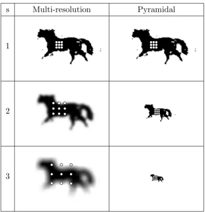
which a label field, resulting from an image classification algorithm, is decomposed and sampled. s Multi-resolution Pyramidal 1 2 3
Figure 3.4: Two examples of multi-scale decomposition and a possible sampling pattern for both. White and black crosses denote the sampling positions.
3.2.1.1 Multi-resolution Decomposition
The Multi-resolution decomposition directly derives from classical multi-resolution the-ory in image processing and analysis. Given y′
Ci(~q), the probability, the marginal, or
the likelihood of the classCiat position~q; we define the multi-resolution decomposition
Φ, as following:
ΦCi(~q;s) =y ′
Ci(~q)∗G(0, γ
s−1) (3.1)
wheres∈ {1,2, . . . , S} represents the scale; ‘∗’ is the convolution operator,Gis a mul-tidimensional Gaussian distribution with zero mean and σ =γs. Here γ is the “step” of the multi-resolution decomposition (typicallyγ = 2). As it can be seen in figure3.4, this methodology, applied on label fields coming from image pixel classification, is mim-icking exactly the well known multi-scale methodology used in image processing and analysis techniques. However here the images represent the probability, the marginal
or the likelihood of a certain class. As a result, the Multi-resolution decomposition provides information regarding the spatial homogeneity and regularity of the label field at different scale. It is easy to understand that, for example, a noisy classification at scale 1 does not influences importantly the results of scale 3. In this way, the highest scale robustly represents the label field in presence of noisy classification (reaching the limit of an almost homogeneous label field) and, at the same time, intermediate scales give different levels of details in the initial label field.
3.2.1.2 Pyramidal Decomposition
An alternative is provided by the pyramidal decomposition (2). The pyramidal de-composition is substantially similar to the multi-resolution dede-composition with the exception that actually, the resulting pyramid codify more efficiently the multi-scale information. However, it has an important drawback that will be discussed in next subsections.
Starting from the above mentioned Multi-resolution decomposition, the Pyramidal decomposition Ψ can be obtained as follows:
ΨCi(~q;s) = ΦCi(⌊kss~q⌋;s) (3.2)
where ⌊·⌋ is the floor function, ~q ∈ NN, N is the dimensionality of the data. Here ~ qj ∈ h 1 Xj γs−1 i
, whereXj is the integer size of every dimension j (for an image,N = 2, X1 andX2are respectively the width and height of the image). Hereksis the sampling
step and depends onγ,ks=γs/2. Actually, the pyramidal decomposition samples the
Multi-resolution theoretically without loss of information, since at higher scales, the high frequency content have been progressively filtered out.
3.2.1.3 Pros and cons of multi-resolution and pyramidal decompositions The multi-resolution approach is the most appropriate in terms of signal processing theory. However, the pyramidal decomposition actually contains the same information as the multi-resolution while coding it in a more compact way. Unfortunately, as it can be noticed in formula (3.5), the sampling at large scales is prone to produce blocking artifacts. This is due to the fact that during the pyramidal decomposition process, each scale summarizes the information of the above area in a block that is γN times smaller (here N is the dimensionality of the data, for images N = 2). Obviously, at large scales this reflects a sharp transition form a value to another in the feature vector. This does not happen using the multi-resolution decomposition, where the Gaussian filtering assures smooth transitions at every scale.
Summarizing, if the input data is sufficiently small, the use of the multi-resolution decomposition is highly recommended, while if the input data is inherently large, the pyramidal decomposition can help to save memory at the cost of possible blocking artifacts. To avoid blocking artifacts, an interpolation technique could be used. How-ever, after the next step, sampling pattern, the resulting output will be the same size, therefore pyramidal decomposition compactness is not a big advantage. For sake of simplicity, our MSSL framework will use the multi-resolution approach as a standard multi-scale decomposition method.
3.2.2 Sampling pattern
Once the desired multi-scale representation has been computed, an appropriate sam-pling pattern should be applied. This pattern can be represented by a set of displace-ment vectors that defines the neighborhoodρ=SMm=1δ~m. Once the displacement
vec-tors are defined, the feature vector for the multi-resolution decomposition is obtained by the following formula:
z(~p) = {Φ(~p+δ~1; 1),Φ(p~+δ~2; 1), . . . ,Φ(~p+δ~M; 1), | {z } scale s=1 Φ(~p+γ ~δ1; 2),Φ(~p+γ ~δ2; 2), . . . ,Φ(~p+γ ~δM; 2), | {z } scale s=2 .. . Φ(~p+γ(S−1)δ~1;S),Φ(~p+γ(S−1)δ~2;S), . . . ,Φ(p~+γ(S−1)δ~M;S) | {z } scale s=S } (3.3)
This formula shows that the sampling is performed following the displacement vectors at each scales. However, the displacement at different scales are multiplied by a factor γ(s−1) so that, higher scales correspond to larger displacement. For the sake of clarity, the sampling in figure3.4(left) is obtained withS = 3,γ= 2,M = 9 and the following set of displacements: ρ={ δ~1 = (−1,−1), δ~2= (−1,0), δ~3 = (−1,1), ~ δ4 = (0,−1), δ~5= (0,0), δ~6 = (0,1), ~ δ7 = (1,−1), δ~8= (1,0), δ~9 = (1,1)}. (3.4)
! δ1 δ!2 δ!3 ! δ4 δ!5 δ!6 ! δ7 δ!8 δ!9 x y
Figure 3.5: A graphical representation of the displacements set ρas defined in formula (3.4)
The feature vector for the pyramidal decomposition can be obtained by the following formula: z(~p) = {Ψ(~p+δ~1; 1), . . . ,Ψ(p~+δ~M; 1), | {z } scale s=1 Ψ(⌊~p/γ⌋+δ~1; 2), . . . ,Ψ(⌊p/γ~ ⌋+δ~M; 2), | {z } scale s=2 .. . Ψ(⌊~p/γ(S−1)⌋+δ~1;S), . . . ,Ψ(⌊~p/γ(S−1)⌋+δ~M;S) | {z } scale s=S } (3.5)
where ⌊·⌋ is the floor function. As in the previous case, the sampling is performed over all the displacements and scales. On the other hand, the position vector ~p is divided by the quantity γ(s−1) to adequately re-scale the coordinates to the resized
images at higher scales. The floor function is needed to obtain an integer vector that lays in the image lattice. The displacement pattern ρ is not modified as the images are progressively smaller at a higher scale. Figure3.4(right) shows an example of this sampling with S = 3, γ = 2, M = 9 and the same displacement set ρ as in formula (3.4).