International Emissions Trading Scheme and European Emissions Trading Scheme : what linkages ?

Documents de Travail du

Centre d’Economie de la Sorbonne

Maison des Sciences Économiques, 106-112 boulevard de L'Hôpital, 75647 Paris Cedex 13 http://ces.univ-paris1.fr/cesdp/CES-docs.htm

International Emissions Trading Scheme and European Emissions Trading Scheme : what linkages ?

Natacha RAFFIN, Katheline SCHUBERT 2007.40

International Emissions Trading Scheme and

European Emissions Trading Scheme: what linkages?

∗

Natacha Raffin

and Katheline Schubert

July 31, 2007

∗_{We thank Mouez Fodha and Philippe Quirion for useful comments and discussion, as well as}

partici-pants to the 7th_{Environmental Economics Meeting. We also thank all the audience of the Environment}

Seminar and Workshop in macroeconomics at Paris I.

†_{Université Paris 1 Panthéon–Sorbonne and Paris School of Economics, 106-112 bd de l’Hôpital, 75013}

Paris, France - Tel: +33 (0)1.44.07.82.13. E-mail address: natacha.raffin@univ-paris1.fr

‡_{Université Paris 1 Panthéon–Sorbonne and Paris School of Economics, 106-112 bd de l’Hôpital, 75013}

Résumé

La concomitance des périodes d’engagement (2008-2012) des marchés internatio-nal et européen de permis pourrait engendrer des distorsions en termes de répartition de la charge environnementale entre les secteurs. En effet, les deux niveaux d’échange (gouvernemental et entrepreneurial) doivent rester cohérents, malgré leurs différentes caractéristiques. Pour atteindre leur objectif, les gouvernements européens devront instaurer une politique additionnelle qui consiste à taxer les émissions des secteurs non-assujettis. La taxe dépendra de l’effort réalisé au sein de l’UE-ETS. Nous pro-posons une modélisation de cette politique à double niveau, en nous concentrant sur le niveau des taxes dans les différents cas d’imbrication. Nous estimons les efforts qui seront demandés aux secteurs non-assujettis ainsi que les différents prix de carbone.

Mots-clef : Protocole de Kyoto, EU-ETS, Coexistence de marchés de permis échangeables domestique et international, prix du carbone et politique environne-mentale.

Codes JEL: Q53 ; Q58 ; Q28

Abstract

Simultaneity between commitment periods (2008-2012) of both International and European Emissions Trading schemes may generate distortions in terms of burden distribution among sectors. There will be two levels of trading (a country and an entity level), which both need to be consistent with one another, despite of their different designs. To reach international targets, European governments will adopt an additional policy. It consists in implementing a tax on emissions of non-covered sectors. The tax rates depend on the effort realized within the European market. We propose a modeling of this two-level environmental policy, focusing on the levels of tax rates in each case of linkage. We obtain empirical estimations of the efforts that could be demanded to non-covered sectors, and of the price(s) of carbon.

Keywords: Kyoto Protocol, EU-ETS, co-existence of domestic and interna-tional emissions trading systems, carbon price, environmental policy.

1

Introduction

Simultaneity between commitment periods (2008-2012) of the International Emissions Trading scheme (hereafter IET) and the European Union Emissions Trading Scheme (hereafter EU-ETS) is likely to generate distortions in terms of distribution of the burden among sectors and among countries. Indeed, the features of these two emissions trading schemes are not the same. The first one is established on a country level whereas the sec-ond one is defined on an entity level. Besides, IET covers sectors not initially included in EU-ETS. To reach international targets, each European government will have to adopt an additional environmental policy concerning these latter sectors. This policy may consist in implementing a tax on emissions of sectors only included in the Kyoto Protocol. The level of such a tax would depend on the effort realized within the European market by the covered sectors. Anyhow, several carbon prices could coexist: an international price, a European price for covered sectors within EU-ETS, and domestic prices –the tax rates– for non-covered European sectors. This would induce distortions in the behavior of firms and states, and would certainly not contribute to the equity and the transparency of the whole carbon device.

We propose in this paper a modeling of this two-level environmental policy, focusing on the additional tax rate that could enable a European government to fulfill its international obligation in presence of a domestic market. It allows us to obtain empirical estimations of the efforts that will be demanded to polluting sectors in European countries, and to show how these efforts would be distributed, under different assumptions about the behavior of Europe on the international market. It also allows us to estimate the different carbon prices that could coexist.

Since February 2005, the Kyoto Protocol on Climate Change has entered into force. It implements an International Emissions Trading Scheme as a mechanism of flexibility to limit greenhouse gas emissions. The first commitment period will start in 2008 and last for five years. The main objective, for Parties members of Annex B1_{, is to reduce the average}

level of emissions by 5.2 percent compared to the 1990 level. Each Party receives a pre-determined amount of allowances (Assigned Amount Units or AAU, expressed in metric tonnes of CO2 equivalent) to fulfill its obligation notified in Annex A of the Treaty. These

units or permits give a right to emit pollutants up to a bounded level. Each government is allowed to sell (or purchase) units on the international market to be in compliance. In this framework, Europe, considered as a “Party”, is required to reduce its emissions level by 8 percent by comparison to the initial level of 1990. In addition, the overall European objective of emissions reduction is distributed among European countries in the “European Burden Sharing Act”.

In spite of the fact that the international market is defined on a country level, the Treaty does not exclude the opportunity of implementing domestic trading systems in or-der to reach targets at least cost, according to Article 17. Thus, according to the Protocol, the European Commission decided in 2003 to implement a domestic environmental

pol-1. Annex B of the Treaty brings together OECD countries participating to the Protocol, plus eastern European countries and ex-soviet block countries, less the United States and Australia.

icy establishing a European Union Emissions Trading Scheme2 (European Commission, 2003). The objective of EU-ETS is to lower the costs of compliance at the international level by gradually reducing emissions, and to enable entities to adapt themselves to a new instrument of environmental policy. This European market is thus established on an entity level. The first commitment period of EU-ETS began in 2005, and the second one will span over the years 2008-2012. Plants included in EU-ETS receive some units called

European Carbon Currency, and can trade them. The European targets within EU-ETS are determined by each European government and reported in the National Allocation Plans. Each NAP is submitted to the approbation of the European Commission.

Hence, both systems will be operating during the same period, 2008-2012. So, there will be two levels of trading during this period: a country level and an entity level, which need to be consistent with one another (Butzengeigeret al., 2001). Each European state will have to respect on the one side the European cap associated with EU-ETS, and on the other side the international target within IET.

However, the designs of these two systems are different. While the international system covers the six main greenhouse gases3_{, EU-ETS covers only CO}

2 emissions. Moreover, the

international market covers sectors not included in the European system such as transport, agriculture, waste and housing-tertiary, in addition to those included in EU-ETS such as energy activities, mineral industries, oil refineries.

In this paper, we focus on the behavior of a European government facing this dou-ble environmental constraint. As mentioned above, within EU-ETS, governments are required to determine the level of emissions reduction, taking into account their inter-national objective. The abatement realized through EU-ETS will be taken into account for the international compliance at the end of the first commitment period, as IET cov-ers emissions of sectors included in EU-ETS. This situation implies a distribution of the burden among covered sectors and sectors only included in IET. As notified by Godard (2005), if the domestic objective is low, then non-covered sectors will have to support the main part of the environmental constraint. Indeed, the presence of a domestic market generates distortions in terms of distribution of the burden both among sectors and among countries.

We consider that European governments will implement a tax rate on emissions of non-covered sectors, to ensure the international compliance. These tax rates will be the instrument that guarantees the linkage between the two systems. They will depend on the burden distribution among sectors, i.e. on the abatement realized within the domestic market compared to the international constraint. But the precise institutional arrange-ments that will prevail are unknown for the moment, so we make several assumptions about the design of the tax system, and study their consequences.

We study in section 2 the behavior of European entities trading on the European

2. European Directive 2003/87/CE, called “Directive PEN” published in the Official Journal of the European Union on October the 13th, 2003.

3. The six main greenhouse gases concerned by the Kyoto Protocol are carbon dioxide (CO2), methane

(CH4), nitrous oxide (N2O), hydrofluorocarbons (HFCs), perfluorocarbons (PFCs) and sulphur

market. We deduce the optimal level of abatement of each country, holding account of the constraints established in the different NAPs. Then, we deal with the consequences of a tax implementation on the behavior of non-covered European entities. We finally study, as a benchmark, the optimal solution, that is to say the initial allocations for covered sectors and the tax rates for non-covered sectors that a European central planner would implement in order to satisfy the Kyoto target at least cost. In section 3, we introduce the International Emissions Trading scheme and describe the behavior of participating countries. We consider three possible cases of linkage. In the first one, a European regulator is the representative actor on the international market; he is able to purchase or sell international permits to ensure the compliance and then he imposes to European countries the same tax rate on their non-covered sectors, equal to the international carbon price. In the second case, there is no European regulator and national governments neglect the possibilities of cost reduction offered by the international market. Then, they fix their own tax rate, to attain their Kyoto objective within the European Burden Sharing Act. Finally, in the third case, a European regulator acts on the international market only and delegates to the countries the task of fixing their tax rate in order to attain the required abatement rate. Section 4 provides numerical estimations of the consequences of the previous assumptions. Finally, we conclude (section 5) by emphasizing the consequences of the current environmental policies and putting forward extensions to the model.

2

Europe

We consider that EU-ETS works independently from IET, over the period 2008-2012. European countries are indexed by k, with k = 1, ..., n. We assume that in a given European countryk, firms belonging to covered sectors can trade permits not only with other covered firms of the same country k, but also with firms of another European country4_{. Each sector is composed of identical firms. Moreover, we assume that European}

sectors are not allowed to engage, for their compliance, units associated with IET, such as project-based mechanisms units (ERUs and/or CERs)5_{. This assumption seems to be}

reasonable, because, at the moment, the amount of CERs and ERUs used by European entities is still marginal.

2.1

Covered sectors: the EUropean Emissions Trading Scheme

The sectors participating to EU-ETS are indexed by j = 1, ..., N. They are the same in all European countries (cf. Annex I of Directive PEN).

4. This assumption is a simplification of reality. In reality indeed, the modeling of intra-European trade requires to define rules about reporting and units conversion. To be consistent with the Kyoto Protocol, trade between European firms in different member-states implies adjustments of countries AAUs amounts (see Carlen, 2004).

5. Industrial trading sectors are allowed to use CERs or/and ERUs for their compliance through the “Linking Directive”, but importation of broad units are limited. ERUs are credits associated to mecha-nisms of Joint-Implementation and CERs are credits associated to Clean Development Mechamecha-nisms.

According to the different NAPs, each sectorj in a given European countryk receives an amount of permits ekj, where PN_j=1ekj = ek 6. A low ekj means of course that the

constraint is stringent, because it represents the level of authorized emissions. The sum over the European countries of the national allocationsekrepresents the overall European

objective: Pn

k=1ek =eets.

It is worth emphasizing that the usual logic of emissions trading systems is reversed here: the European countries decide on their own initial endowmentek, and the addition

of these decisions determines the overall constrainteets.The incentive for each European

country not to choose an initial allocation equal to its business-as-usual emissions comes from the threat of the European Commission not to approve its NAP (see the case of the French NAP in December 2006).

Lete0

kjbe the business-as-usual (BAU) emissions of sectorj in countryk,i.e. emissions

without any environmental policy. Total BAU emissions within EU-ETS for covered sectors are Pn

k=1 PN

j=1e 0

kj = e0ets. Moreover, akj is the abatement of sector j in country

k. The remaining emissions after abatement are e0_kj −akj.

The effort of abatement akj provided by a sector j induces a cost Ckj(akj). The

abatement cost function is supposed twice differentiable and strictly convex: C_kj0 (akj)>0

andC_kj00 (akj)>0. Abatement cost functions can differ among sectors and across countries

because levels of technology are different (Jacoby and Wing, 1999).

Each sector j has to buy (or can sell) European permits at a competitive price pe to

fill the gap between emissions after abatement and its quantified target.

Then, each covered sector j seeks to minimize its compliance costs, by determining the optimal level of abatement:

min

akj

Ckj(akj) +pe[(e0kj−akj)−ekj] ∀j = 1, ..., N and ∀k = 1, ..., n. (1)

The first order condition yields

C_kj0 (akj) = pe ∀j = 1, ..., N and ∀k= 1, ..., n. (2)

So, as it is well known, the marginal abatement costs are equalized in each sector of each country participating to the European market, and the common marginal abatement cost equals the price of permits.

The equilibrium on the European permits market states that the sum of effective emissions after abatement is equal to the emission cap:

n X k=1 N X j=1 (e0_kj−akj) =eets. (3)

It allows us to obtain the price of permits. It can also be written as follows:

n X k=1 N X j=1 akj =e0ets−eets. (4)

6. The initial allocation is given to European sectors by grandfathering, i.e. without charge and in proportion of their past emissions and their growth expectations.

The right-hand side member of equation (4) is the effort in terms of emissions reduc-tion peformed by covered European sectors, and the left-hand side member is the total abatement realized within EU-ETS.

2.2

Non-covered sectors: taxation

We consider here polluting sectors which are not included in EU-ETS. Their greenhouse gas emissions are however involved for the international compliance within the Kyoto Protocol. So, we assume that each European government implements an additional en-vironmental policy, here a tax on emissions, in order to satisfy the international objec-tives. These sectors are specifically transport, and others, such as agriculture, waste and housing-tertiary. They are mainly emitters of non-point source pollution, and for this reason can hardly be included in EU-ETS. This justifies the choice of taxation for reg-ulating their emissions. The coexistence of a domestic and an international emissions trading schemes, i.e. of two environmental policy instruments, implies a distribution of the burden among sectors. If the effort realized within the domestic market by covered sectors is low, then obviously the tax rate imposed on non-covered European sectors will be high, in order to respect the commitments.

Non-covered sectors in each European country k are indexed by h = 1, ..., M. τk

denotes the tax rate on the emissions of these sectors. We assume a single tax rate on all non-covered sectors, in line with the usual implemented fiscal policies. It is exogenous for non-covered sectors, but will be determined by each government in order to comply with its international obligations.

The abatement of non-covered sectors in a given European country k is bkh, with

P

hbkh = bk, and the baseline emissions fkh0 , with

P

hfkh0 = fk0. Emissions after

abate-ment are then(f_kh0 −bkh). Dkh(bkh)denotes the abatement cost function, supposed twice

differentiable and convex: D_kh0 (bkh) > 0 and Dkh00 (bkh) > 0. Non-covered sectors seek to

minimize their costs by choosing the level of abatement:

min

bkh

Dkh(bkh) +τk(fkh0 −bkh) ∀h= 1, ..., M and ∀k= 1, ..., n. (5)

Writing the first order condition yields the usual equality between marginal abatement costs and the tax rate:

D_kh0 (bkh) =τk ∀h= 1, ..., M and ∀k= 1, ..., n. (6)

2.3

Benchmark: the optimal solution

We assume the existence of a European central planner who seeks to minimize the total abatement cost of the European Union, for a given Kyoto commitment eEk for each

European countryk. We want to calculate the efficient global constraint that should be imposed on covered sectors, and the optimal carbon price. We assume that non-European countries express a given net demand of permits on the Kyoto marketεK_i , exogenous from the point of view of the European central planner.

The abatement of a covered sector j in a European country k is by definition equal to the difference between its BAU emissions and the sum of its initial allocation of permits and its purchase (sell) of European permits, denoted εkj, with εkj T0:

akj =e0kj −(ekj+εkj). (7)

The total abatement of covered sectors of country k is then:

X j akj = X j e0_kj −X j ekj− X j εkj =e0k−ek− X j εkj. (8)

The abatement of non-covered sectors in a country k allows it to comply with its Kyoto commitment. For this, it is necessary that the total abatement of country k equals the difference between its BAU emissions and its Kyoto commitment eEk augmented by its

purchases of European permits and of Kyoto permits, denoted εK_k:

X j akj+ X h bkh =e0k+f 0 k − eEk+ X j εkj+εKk ! . (9)

Equations (8) and (9) allow us to obtain the abatement of non-covered sectors of country

k: X h bkh =fk0+ek− eEk+εKk . (10)

The constraints that must hold are the following:

X k X j εkj = 0, (11) X k εK_k +εK_i = 0, (12)

meaning that the sum of net purchase of permits must be equal to zero on the European market and on the Kyoto market as well.

Efficiency requires the minimization of the total abatement cost:

min εkj,ekj,εKk X k X j Ckj(akj) + X h Dkh(bkh) ! , (13)

with respect to constraints (11) and (12).

Letp1 and p2 be the shadow carbon prices on each market. The first order conditions

of the European planner’s program yield:

C_kj0 (akj) =p1 =Dkh0 (bkh) =p2 ∀k, j and h. (14)

The efficient solution then consists in a single carbon price (p∗ = p1 = p2), and in the

is then possible to obtain the efficient global constraint e∗_ets that should be imposed on covered sectors in order to satisfy these conditions, for any given net demand of Kyoto permits by non-European countries.

This solution will be used as a benchmark in the numerical exercises performed below, and we will in particular evaluate the departure of the actual initial allocations from the efficient ones.

The next section describes the IET scheme. The overall objective to respect is a European objective (a reduction of 8% compared to the level of emissions in 1990), which is then shared among European countries. The behavior of each European government on this market will provide the additional tax rate to be implemented.

3

The International Emissions Trading scheme

The IET scheme will run from 2008 to 2012 and is established on a country level: gov-ernments are responsible for their compliance. Annex B Parties will have to reduce by 5.2 % their average level of emissions (compared to the base year, 1990) over the period. Parties participating to the international permits market are able to trade AAUs to be in compliance.

We consider that each Party is price taker and that the international market is com-petitive. p denotes the price of international permits.

In addition, we assume that the IET scheme is represented by two agents considered as two zones: “Europe”, indexed byE, and the “Rest of the Parties”, indexed by i7_.

These two zones must respect an international “cap” e. The free initial allocations of permits for each zone areeE and ei, witheE+ei =e. Hence,e corresponds to the global

international objective of 5.2 % in average over the period 2008-2012.

3.1

The Rest of the Parties

Let e0

i denote the baseline emissions for the Rest of the Parties. Zone i has to fulfill its

commitmentei by reducing its polluting emissions or trading on the market. Notice that

for zone i, all polluting sectors stated in the Kyoto Protocol are included. There is no distinction among sectors. The abatement of zone i is ai and the remaining emissions

after abatement are (e0

i −ai).

As for other Parties, the activity of cleaning up is associated with a twice differentiable, increasing and convex abatement cost functionKi(ai), where Ki0 >0 and K

00

i >0.

Zone i minimizes its compliance costs:

min ai Ki(ai) +p (e0_i −ai)−ei , (15) yielding as usual: K_i0(ai) =p. (16)

7. Bulgaria, Canada, Japan, Liechtenstein, Norway, New-Zealand, Romania, Russian Federation and Switzerland compose the “Rest of the Parties”.

3.2

Europe

Europe as a whole must respect its overall objective eE,where the objective of each

Eu-ropean countryeEk is set in the European Burden Sharing Act. The current institutional

arrangements, and in particular the fact that Europe is considered as a single zone, seem to suggest that the European actor on the market of international permits will be a sin-gle European entity, that we name the European regulator. Nevertheless, we study here differentscenari concerning the potential behavior of European countries on the interna-tional market, and compare their consequences. We assume that European constraints for covered sectors are given, while the tax rates imposed on non-covered sectors are still undetermined. Then, the tax rate must compensate the difference between European emissions of covered sectors and the international European objective.

3.2.1 European regulator able to impose the national tax rates

Suppose first that there exists a European regulator able to impose to European gov-ernments the tax rates they must apply to their non-covered sectors. Then, obviously, he will impose in each European country a tax rate on emissions of non-covered sectors equal to the price of an international permit8_{, given that this price reflects the global}

environmental constraint:

τk =p ∀k. (17)

The abatement of non-covered sectors in a country k is then bkh = D0−kh1(p). Everything

goes as if the non-covered sectors of all European countries were allowed to trade permits directly on the international market, and the equilibrium of the market is, in terms of abatements: ai+ n X k=1 M X h=1 bkh = e0−e − e0_ets−eets . (18)

The abatement of the Rest of the Parties and of the European non-covered sectors is equal to the difference between the global Kyoto effort e0−e and the effort realized by the European covered sectorse0

ets−eets.

This solution is not very plausible. Fixing the tax rates is still a state prerogative, that will not be so easily given up to the European regulator, all the more so since the determination of the NAPs remains a domestic prerogative.

3.2.2 National regulators fixing their own tax rates

So let us consider now that each national regulator does not take into account opportu-nities provided by the international market. It implies that each European government determines its own tax rateτk, in order to reach its Kyoto target eEk, the effort realized

by the covered sectors being considered as given.

8. This simple static set-up prevents from taking into account the fact that a tax rate is fixed for a certain time length, while a market price varies daily. In a more general set-up, the tax rate should be a mean of the carbon market prices.

For European countryk,the iso-abatement curve associated with the abatement objec-tivee0

k+fk0−eEkgives the relationship between the tax rate supported by the non-covered

sectors and the level of the constraint imposed on covered sectors. It can be written as follows: N X j=1 akj+ M X h=1 bkh =e0k+f 0 k −eEk, (19)

or, the abatement levels akj and bkh being given by the first order conditions (2) and (6)

and the price of European permits by equation (4):

N X j=1 C0−_kj1(pe) + M X h=1 D0−_k1(τk) =e0k+f 0 k −eEk, (20) with n X k=1 N X j=1 C0−_kj1(pe) = e0ets−eets. (21)

We can see that the weight of the initial allocation ek of a given European country k in

its iso-abatement curve is “diluted” in the global constraint eets through the European

market. Every country is then incited to propose to the European Commission a NAP assigning an effort to its covered sectors as small as possible, hoping that the others will do the job without enforcing it to increase the tax rate τk to meet a given abatement

objective.

The obvious drawbacks of this solution is that Europe does not take advantage of the international market to reduce its abatement costs. Its merit is that each European country remains sovereign as far as its fiscal policy is concerned.

3.2.3 European regulator acting on the international market only

We suppose now that there exists a European regulator whose job is to determine jointly the total European rate of abatement and the net purchases of international permits, given the Kyoto constraint on European emissionseE.

Lete0

E denote the total European BAU emissions. They are the sum of the emissions

of covered and non-covered sectors:

e0_E = n X k=1 e0_k+ n X k=1 f_k0 =e0_ets+ n X k=1 f_k0. (22)

To determine the total level of abatement, the European regulator minimizes its com-pliance costs. We suppose that he uses an aggregate abatement cost function for Europe

K(aE).The relationship between the sectoral cost functions and this aggregate cost

func-tion is given in the Appendix. Thus, the program of cost minimizafunc-tion for the European regulator acting on the international market is written as follows:

min

aE

KE(aE) +p[ e0E−aE

and the first order condition yields:

K_E0 (aE) = p. (24)

The competitive price of an international permit is given by the equilibrium on the market:

ai+aE =e0 −e, (25)

whereai and aE are given by the first order conditions (16) and (24).

This total European abatement effort within the IET decided by the European regu-lator is also the sum of the abatement efforts of the n European countries:

aE(p) = n X k=1 N X j=1 akj(pe) + M X h=1 bkh(τk) ! , (26)

whereaE(p)is given by equation (24), akj(pe)by equation (2) andbk(τk)by equation (6).

As we assume that allocations for covered sectors are given, then each tax rate must be calculated in a way to satisfy equation (26). Obviously, a unique tax rates system solution of this equation does not exist. A constraint must be added, describing the sharing of efforts among the European countries, which could be proportional to their emissions reduction objective of theEuropean Burden Sharing Act. We would then have

aEk(pe, τk)

eEk

= aE(p)

eE

, (27)

which allows us to obtain τk knowing pe and p.

4

Simulations

We simulate now the previous model, and determine for every European country the tax rate that should be implemented and the resulting abatement for covered and non-covered sectors.

4.1

The tax rates for quadratic abatement cost functions

The assumptions made for the characteristics of the abatement cost functions –convexity and degree of steepness– are very important. We consider a quadratic abatement cost function because it is convex, it yields linear marginal abatement costs, which greatly simplifies the simulations, and finally there is no convincing argument in the literature to do otherwise.

Sectoral abatement cost functions are then

Ckj(akj) = αkj 2 a 2 kj, (28) Dkh(bkh) = βkh 2 b 2 kh. (29)

Parameters αkj >0 and βkh > 0 represent the levels of abatement technology, which

differ between countries and between sectors. The more malleable the production process, the lower the parameter, and the lower the cost of reduction of pollution (Jacoby and Wing, 1999). Opportunities of substitution in the production process, i.e. substitution between polluting and clean inputs, are thought to be more important for covered sectors, in particular for energy.

We can deduce through the first order conditions (2) and (6) that

akj = pe 1 αkj , (30) bkh = τk 1 βkh , (31)

and the equilibrium of the market for emission permits (4) yields:

pe= e0 ets−eets Pn k=1 PN j=1 1 αkj . (32)

We can now calculate the tax rates on non-covered European sectors in the different cases studied above.

4.1.1 Benchmark

We must find the optimal carbon price and the initial global constraint e∗_ets that lead to the equalization of all the marginal abatement costs, for covered and non-covered sectors, in every European country, given the international demand for permitsεK

i and the Kyoto

commitmentseEk.

The international demand of permits is of course related to the level of abatement of non-European countries: εK_i =e0_i −ai−ei. (33) Equation (9) reads: p X j 1 αkj +X h 1 βkh ! =e0_k+f_k0− eEk+ X j εkj+εKk ! , (34)

and the sum of these equations over all European countries combined to the equilibrium constraints and the preceding expression ofεK

i gives: pX k X j 1 αkj +X h 1 βkh ! =X k e0_k+f_k0−eEk +e0_i − p γi −ei =e0 −e− p γi . (35)

The optimal carbon price is then:

p∗ = e 0 _−e 1 γi + P k P j 1 αkj + P h 1 βkh . (36)

This allows us to obtain the abatements a∗_kj = p∗/αkj, b∗kh = p ∗_/β kh, a∗i = p∗/γi, as well as (ekj+εkj) ∗ = e0_kj − p ∗ αkj (37) ek−εKk ∗ = eEk−fk0+p ∗X h 1 βkh , (38)

and, by summing over all sectors and all European countries,

e∗_ets =e0_ets−pX k X j 1 αkj . (39)

Equation (39) gives the optimal total constraint on covered sectors within EU-ETS. Equation (38) shows that the optimal constraint for each European country is not de-termined uniquely: what is unique is the difference between this constraint and the net purchase of Kyoto permits by the country. It is the same at a sectoral level (equation (37)).

4.1.2 European regulator able to impose the national tax rates

We then havebkh = _βp_kh, and equation (18) yields:

p=τk = (e0_−e)−(e0 ets−eets) 1 γi + P k P h 1 βkh . (40)

We can see easily that this carbon price is the same as the optimal one given by equation (36) if and only if the global constraint on the European market is such that

e0 ets−eets P k P j 1 αkj = e 0_−e 1 γi + P k P j 1 αkj + P h 1 βkh , (41)

i.e. if the distribution of the efforts of abatement is the same in the European market and in the Kyoto market.

4.1.3 National regulators fixing their own tax rates

Then, equation (20) yields:

τk = e0_k+f_k0−eEk−(e0ets−eets) P j_αkj1 P k P j 1 αkj P h 1 βkh . (42)

4.1.4 European regulator acting on the international market only

We show in the Appendix that the aggregate cost function for Europe is also quadratic, and can be written

K(aE) = γE 2 a 2 E, (43) with γE = 1 P k P j 1 αkj + P h 1 βk . (44)

We can then easily deduce from equation (27) the tax rates in the quadratic case:

τk= p_γ1 E eEk eE −pe P j 1 αkj P h 1 βkh , (45)

pbeing given by the equilibrium condition on the international permits market (equation (25)): p= e 0_−e 1 γi + 1 γE , (46)

which finally allows us to obtain

τk= 1 P h 1 βkh e0−e 1 γi + 1 γE 1 γE eEk eE − e 0 ets−eets P k P j 1 αkj X j 1 αkj ! . (47)

4.2

Simulations

For European countries, the data used for the simulations come from the European Pol-lutant Emission Register9_{, from the estimated NAPs for 2008-2012 and finally from the}

data of the POLES model (Criquiet al, 2003). We obtain BAU emissions for 2010, for all covered sectors, the allocations per year and also the environmental constraints. More-over, we use BAU data for non-covered sectors and other countries participating to the international emissions trading scheme. We use specifically data from the national reports submitted to the UNFCCC10_{. European covered sectors are: energy activities (refining,}

other combustion activities), production and processing of ferrous metals, mineral indus-try (cement, glass, lime, ceramics products...) and chemical indusindus-try, pulp and paper production and manufacturing industries and construction.

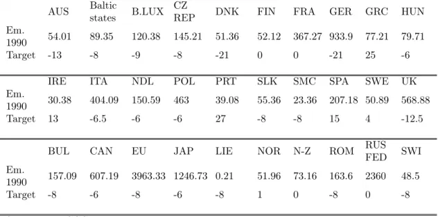
We assume that there are two representative non-covered sectors. The first one is transport, and the second one includes agriculture, housing-tertiary, wastes and other industrial sectors not included in the preceding list. Table 1 gives total greenhouse gas emissions (in Mt CO2 equivalent) for the base year 1990, as considered by the Kyoto

Protocol, and Kyoto’s targets for 2008-2012, for European countries and the Rest of the Parties.

9. http://www.eper.cec.eu.int 10. http://www.unfccc.int

Table 1. Greenhouse gas emissions (Mt eqCO2) and international environmen-tal target (%) under the Kyoto Protocol

AUS Baltic

states B.LUX CZ

REP DNK FIN FRA GER GRC HUN

Em.

1990 54.01 89.35 120.38 145.21 51.36 52.12 367.27 933.9 77.21 79.71

Target -13 -8 -9 -8 -21 0 0 -21 25 -6

IRE ITA NDL POL PRT SLK SMC SPA SWE UK

Em.

1990 30.38 404.09 150.59 463 39.08 55.36 23.36 207.18 50.89 568.88

Target 13 -6.5 -6 -6 27 -8 -8 15 4 -12.5

BUL CAN EU JAP LIE NOR N-Z ROM RUS

FED SWI Em. 1990 157.09 607.19 3963.33 1246.73 0.21 51.96 73.16 163.6 2360 48.5 Target -8 -6 -8 -6 -8 1 0 -8 0 -8 Source: UNFCCC. 4.2.2 Calibration

The most important point for our purpose is the calibration of the parameters of the marginal abatement cost functions. Unfortunately, estimates of marginal abatement costs vary widely in the literature. These estimates are usually obtained by simulation of a model, and the structural modeling choices greatly impact the results. Following the IPPC framework (Fischer and Morgenstern, 2006), four main factors contribute to vari-ances in estimates: the projections of base case emissions, the structural characteristics of the model (sectoral and technical detail, optimization techniques, functional forms...), the climate policy regime considered and finally the consideration of adverted climate damages. After data on marginal abatement costs have been obtained by simulation, these data are fitted to a chosen specification of the abatement cost function, allowing to obtain the parameters of this function. Finally, we need here not only estimates of aggregate marginal abatement costs, but also sectoral data, more difficult to obtain.

This article uses estimates provided by the POLES model (Criquiet al, 2003). POLES is a bottom-up model, with elaborated data concerning different polluting sectors, specific levels of technology and recent projections of business-as-usual emissions. We consider here five main sectors covered by EU-ETS, which are chemistry, electricity, mineral in-dustry, industry of ferrous metals and finally other industries such as pulp and paper. We use POLES to determine the technological parameters included in the abatement cost functions. More precisely, POLES calculates the level of emissions in 2012 in terms of spread (expressed as a percentage) compared to the constraint, for a carbon price ranging from0to42e. Thus, we calculate the parameters values through these estimated values

of emissions11. Table 2 gives the results of the calibration.

Table 2. Estimated technological parameters

Gbr Fra Ita Ger Esp Grc Prt BLN Swe Pol Hun New

count. other count. covered Chem. 2.51 0.67 2.46 0.29 0.78 61.19 6.56 1.78 27.72 0.93 34.86 27.72 46.27 (αkj) Steel 1.64 1.48 1.36 9.53 2.72 274.7 622.6 2.35 1.60 1.48 23.09 28.54 41.55 NMM 51.89 12.27 4.16 9.53 2.21 7.06 3.08 53.06 96.15 27.89 166.4 328.8 115.6 Other in-dus. 0.31 0.44 0.24 0.12 0.38 0.95 1.69 3.49 1.51 1.31 10.38 11.35 3.50 Elec. 0.09 0.21 0.12 0.05 0.10 0.35 0.71 0.41 3.63 0.13 1.51 1.46 0.75 non-covered Trans. 0.11 0.11 0.15 0.11 0.11 0.59 0.51 0.39 0.72 0.93 1.27 2.86 1.08 (βkh) Others 0.20 0.20 0.24 0.17 0.41 1.12 2.45 0.62 8.39 0.75 2.13 9.01 3.01

Source: POLES model and own calculations. BLN : Belgium, Luxembourg, Netherlands.

New countries : Baltic States, Czech Republic, Cyprus, Malta, Slovakia, Slovenia. Other countries: Austria, Denmark, Finland, Ireland.

Our assumption of linear marginal costs is clearly very rough: all the differences among sectors and across countries in terms of technologies, possibilities of substitution between dirty and clean inputs, efforts already done to adopt cleaner production processes... are embodied in a single parameter. For instance, a high value of the parameter of the marginal abatement cost suggests that the opportunities of substitution are low. This can be due either to the fact that some sectors or some countries have already done important efforts by developing cleaner technologies (electricity sector in Sweden for instance), or to the fact that some others do not have any available clean processes of production.

4.2.3 The tax rates and abatements

We present now the results of the different simulations. They are very sensitive to the value of the parameterγi,the level of technology used in the cost abatement function for

zone “Rest of the Parties”. In the absence of information which could have helped us to make a better choice, we suppose here thatγi is equal to the calibrated value of γe.

The exogenous variables are given in tables 3 and 4. Their values result from the data of the United Nations Framework Convention on Climate Change (figures reported in national submissions) and from POLES data (concerning baseline emissions of covered sectors).

11. We calculate parameters on estimated values because so far there is no data about the abatement realized through the carbon market for European countries, this instrument being too recent.

Table 3. Exogenous variables (Mt eqCO2

e0

ets eets eE e0E ei e0i e0 e γi

2339.7 2083.6 3645.9 4944.6 4568.2 4667.4 9612.02 8214 0.005 Source: UNFCCC and POLES.

Table 4. Initial allocations to covered sectors (¯ekj)

Gbr Fra Ita Ger Esp Grc Prt BLN Swe Pol Hun New

count. other count. Chem. 10.1 13.2 10.4 6.2 6.5 0.8 1.0 23.3 2.0 7.9 3.5 7.6 2.2 Steel 19.9 27.5 23.3 37.4 9.7 1.5 0.4 24.0 8.1 18.6 3.4 29.3 15.9 NMM 17.2 21.8 37.4 51.2 33.1 12.5 8.6 15.3 5.2 19.9 5.0 19.0 14.0 Oth. ind. 8.9 19.6 4.8 3.4 4.4 1.3 0.3 11.9 2.3 11.7 0.3 4.6 7.4 Elec. 167.7 62.1 127.1 358.8 93.2 54.4 24.8 69.4 6.9 216.8 23.6 150.0 74.9 total 223.7 144.2 203.0 456.9 146.9 70.3 35.1 144.0 24.5 274.9 35.9 210.5 114.4 Source: POLES.

Table 5 gives the results of the benchmark simulation. We calculate the single carbon price (p∗ = 3.5e/teq CO2), and the optimal global constraint on European covered sectors

(e∗_ets = 1895.5Mt eqCO2). Notice that this constraint is about 10% lower than the actual

one (eets = 2083.6 Mt eqCO2), which supports the analysis of many observers stressing

that the allocations within EU-ETS are too lenient (see for instance Godard 2005). We then deduce the levels of abatement for each sector in each European country and for the “Rest of the Parties”. The abatements are reported as a percentage of BAU emissions, to have a measure of the efforts demanded to the different sectors in the different countries. Marginal costs of abatement are equalized in the benchmark. Nevertheless, the results show that non-covered sectors and especially transport would have to assume an important part of the burden. As for covered sectors, electricity would have to fulfill the main part of the commitment. At a country level, Sweden, which is well-known as an environmentally friendly country, would have to do a low effort to reach its target, except in the steel sector, compared to France, Germany or United Kingdom. Moreover, the generous Kyoto targets in Eastern Europe countries (“hot air”) introduce variances between levels of abatement among countries. Finally, we calculate the abatement for zone “Rest of the Parties”:

ai = 699.10Mt eqCO2, that is to say 16% of BAU emissions.

We now examine the three potential cases of linkages, focusing on the discrepancy of abatement levels, tax rates and permit prices. Notice that from now on, the national European constraints are determined ex ante. Table 6 reports the abatement efforts of

Table 5. Abatement efforts in the benchmark case (% of BAU emissions),

p∗ = 3.5 e/teq CO2

Gbr Fra Ita Ger Esp Grc Prt BLN Swe Pol Hun New

count. other count. covered Chem. 10.1 24.1 10.6 44.4 35.8 8.1 23.8 16.7 13.0 26.9 5.9 32.8 19.3 (a∗_kj) Steel 11.6 15.3 14.3 0.9 16.3 7.5 4.7 16.6 57.5 12.2 5.3 6.8 23.8 NMM 1.7 3.5 5.6 2.7 9.8 10.1 17.6 3.8 3.2 2.7 2.0 2.8 8.8 Oth. ind. 30.8 28.0 57.5 92.5 46.1 68.4 45.5 20.4 33.3 18.6 15.2 50.7 23.7 Elec. 15.3 18.7 18.4 15.0 25.3 17.7 21.7 19.0 11.5 12.2 10.8 14.4 20.0 non-covered Trans. 20.6 20.8 19.3 18.1 29.5 25.0 33.7 24.9 20.8 14.6 24.2 26.9 26.4 (b∗_kh) Others 4.7 7.2 10.5 6.0 5.8 8.1 5.0 13.4 2.5 3.4 4.2 2.7 5.1

European covered sectors within EU-ETS. The European carbon price is pe = 2 e/teq

CO2. It is much lower than the benchmark carbon price (p∗ = 3.5 e/teq CO2). Then,

obviously, the carbon prices for non-covered sectors will be higher, whatever the behavior of the European regulator.

Table 6. Abatement efforts of covered sectors within EU-ETS (% of BAU emissions), pe= 2 e/teq CO2

Gbr Fra Ita Ger Esp Grc Prt BLN Swe Pol Hun New

count. other count. Chem. 5.8 13.9 6.1 25.6 20.7 4.6 13.7 9.7 7.5 15.5 3.4 18.9 11.1 Steel 6.7 8.8 8.3 0.5 9.4 4.3 2.7 9.6 33.2 7.1 3.1 3.9 13.7 NMM 1.0 2.0 3.2 1.6 5.6 5.9 10.2 2.2 1.8 1.5 1.2 1.6 5.1 Oth. ind. 17.8 16.1 33.2 53.3 26.6 39.4 26.3 11.8 19.2 10.7 8.8 29.2 13.7 Elec. 8.8 10.8 10.6 8.7 14.6 10.2 12.5 11.0 6.7 7.1 6.2 8.3 11.5

Table 7 reports the abatement efforts of European non-covered sectors in the case where there exist a European regulator able to impose the national tax rates. Remember that in this case, everything goes as if the non-covered sectors were allowed to act on the international market. The tax rates are equal to the international permit price, p = 4.1

e/teq CO2. The carbon price is then higher for non-covered sectors than for covered ones.

We observe a great variance in the required levels of abatements for non-covered sec-tors. Transport generally supports the main part of the burden.

higher effort demanded to the “Rest of the Parties”: ai = 802.2 Mt eqCO2, reflecting a

reduction by 19% of BAU emissions.

Table 7. Abatement efforts of non-covered sectors (% of BAU emissions) in the case where the European regulator is able to impose the national tax rates, p= 4.1 e/teq CO2

Gbr Fra Ita Ger Esp Grc Prt BLN Swe Pol Hun New

count. other count. Trans. 24.1 24.4 22.6 21.3 34.6 29.3 39.4 29.4 24.4 17.1 28.3 31.5 30.9 Others 5.5 8.4 12.3 7.1 6.8 9.5 5.9 15.8 3.0 4.0 4.9 3.1 6.0

We study now the situation where national European regulators do not take into account the international system. We find the different tax rates imposed on non-covered sectors (table 8).

Table 8. Tax rates and abatement efforts (% of BAU emissions) in the case where national regulators fix their own tax rate

Gbr Fra Ita Ger Esp Grc Prt BLN Swe Pol Hun New

count. other count. τk 21.7 13.1 7.7 17.6 15.5 10.1 13.1 6.5 2.7 0.0 1.9 5.7 18.6 Trans. 127.7 77.7 42.7 91.2 130.3 72.5 46.6 43.1 16.1 0.0 12.8 46.8 128.1 Others 29.3 26.8 23.3 30.4 25.7 23.6 25.1 20.9 2.0 0.0 2.2 4.6 24.6

The main result here is that the tax rates are in general much higher than the European permit price paid by covered sectors, but also much higher than the unique tax rate of the previous simulation. It means that when countries do not take into account the opportunities provided by the international market they transfer a huge part of the burden to non-covered sectors. Acting on the international market enables entities to share the effort through trade. This case is then characterized by great distortions among sectors. Tax rates greater than 100% occur for transport in Great Britain and Spain, meaning that these sectors must reduce their emissions to zero, which can only be achieved by a complete change of technology. Moreover, the global effort is not fairly allocated among countries. Eastern European countries are required to do a relatively low effort, because of their low Kyoto constraint. Poland for instance can achieve its Kyoto commitment without implementing any additional environmental policy. On the contrary, the high levels of tax rates suggest that the “old European countries” should make an important

additional effort to ensure compliance. The case of Spain is interesting and underlines the fact that EU-ETS allocations are sometimes not adapted: actually, the tax rate to impose is high, while this country has an international objective of reduction which is positive (+15%compared to 1990). It means that expected BAU emissions will widely exceed the Kyoto constraint.

To conclude, this case of linkage seems to be the less desirable. Indeed, to reach the same target, non-covered European sectors would have to support very high tax rates, which would intensify sectoral distortions.

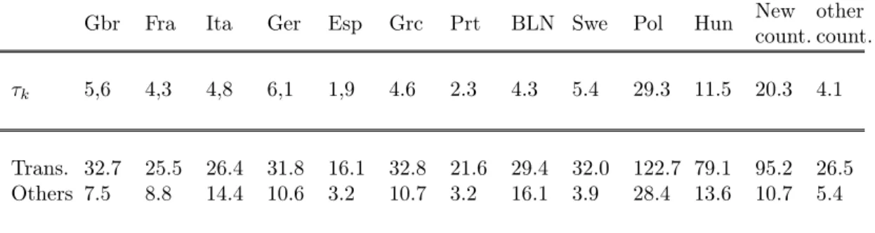
Finally, we study the case where the European regulator acts on the international market. We still deduce the different tax rates, the levels of abatement for covered sectors, non-covered sectors and for the Rest of the Parties and a new international permit price (table 9).

Table 9. Taxation and abatement efforts of non-covered sectors (% of BAU emissions) when a European regulator acts on the international market, p= 3,5e/teqCO2

Gbr Fra Ita Ger Esp Grc Prt BLN Swe Pol Hun New

count. other count. τk 5,6 4,3 4,8 6,1 1,9 4.6 2.3 4.3 5.4 29.3 11.5 20.3 4.1 Trans. 32.7 25.5 26.4 31.8 16.1 32.8 21.6 29.4 32.0 122.7 79.1 95.2 26.5 Others 7.5 8.8 14.4 10.6 3.2 10.7 3.2 16.1 3.9 28.4 13.6 10.7 5.4

Notice that the international permit price is the same as in the benchmark situation, while the European permit price for covered sectors is lower. The tax rates imposed on non-covered sectors are in average higher than both the European and the international permit price. Despite trade between the “Rest of the Parties” and the European non-covered sectors, the burden on European non-non-covered sectors is still large. This is merely induced by too lenient European allocations. The main qualitative difference between this case and the previous one is the effort demanded to the non-covered sectors of the Eastern European countries. As this effort is nil or very low in the previous case, it is high here, because the mechanism of allocation of the effort does not allow them to take advantage of the hot air. On a global level, the European regulator may shift the environmental burden on the less technologically advanced countries, in order to stimulate technological innovation.

5

Concluding remarks

To fulfill their international commitments, European governments will have to implement a tax rate on initially non-covered sectors. The main message of the paper is that if

the allocations granted to covered sectors continue to be globally too lenient, the burden imposed on non-covered sectors (among which transport mainly) and the distortions be-tween sectors and countries will be important. Moreover, the precise way of determining the tax rates will have a great impact. It is essential to take advantage of the international market, which allows to alleviate through trade the burden on non-covered sectors.

The first important extension of the model would be the introduction of project mecha-nisms (Clean Development Mechamecha-nisms and Joint Implementation). These opportunities are not yet used extensively, but they will in the future be the clue of the consistent coexistence of the two systems.

Another interesting extension would be to abandon the assumption of a competitive international market, and to introduce a possible market power of the European Union or of some Parties, such as Russia which benefits from “hot air”.

References

Bréchet, T. and Michel, P. (2005),“Markets of tradable permits when firms are heterogenous”,

mimeo.

Butzengeiger, S., Betz, R. and Bode, S., Hambourg Institute of International Economics (2001).

Making ghg emissions trading work. Crucial issues in designing national and international emis-sions trading systems.

Carlen, B., Department of Economics, Stockholm University. (2004). EU’s emissions trading system in the presence of national emission targets.

Criqui, A., Kitous, A. and Stankeviciute, L. (2003),“The fundamentals of the Future International Emission Trading Systems,” mimeo.

European Commission (2003), Directive 2003/87/EC of the European Parliament and of the Council establishing a scheme for greenhouse gas emission allowance trading within the Commu-nity and amending Council Directive 96/61/EC.

European Commission (2004), Directive 2004/101/EC of the European Parliament and of the Council, amending Directive 2003/87/EC establishing a scheme for greenhouse gaz emission allowance trading within the Community, in respect of the Kyoto Protocol’s project mechanisms.

Fischer,C. and Morgenstern, R. (2006),“Carbon Abatement Costs: Why the Wide Range of Estimates? ” The Energy Journal 27(2):73–86.

Georgopoulou, E., Sarafidis, Y., Mirasgedis, S. and Lalas, D.P. (2006),“Next allocation phase of the EU emissions trading scheme: How tough will the future be?” Energy Policy 34: 4002-4023. Godard, O. (2005),“Politique de l’effet de serre ; une évaluation du plan francais de quotas de CO2.” Revue Française d’Economie, 19:147-186.

Jacoby, H. and Wing, I. S. (1999), “Adjustment time, capital malleability and policy cost.” Special issue The costs of the Kyoto Protocol, The Energy Journal, 73-92.

Mission Interministérielle de l’Effet de serre (2004), Ministère de l’Ecologie et du Développement Durable. Plan Climat 2004.

Appendix: the aggregate abatement cost function

We define the aggregate abatement cost function for any abatement a as the minimum of the sum of the sectoral abatement costs functions for all European countries, given that the sum of sectoral abatements is equal to the aggregate abatement (see for instance Bréchet and Michel, 2005):

KE(a) =    minP k P jCkj(akj) + P hDkh(bkh) a=P k P jakj+ P hbkh .

The Lagrangian of this program is:

L=X k X j Ckj(akj) + X h Dkh(bkh) ! +λ " a−X k N X j=1 akj + X h bkh !# ,

and the first order conditions yield:

λ =C_kj0 (akj) =D0kh(bkh).

We then obtain the sectoral abatements as functions of the Lagrange multiplier λ:

b akj = Ckj0 −1 (λ) bb_kh = D0_kh −1 (λ) b a = X k X j C_kj0 −1(λ) +X h D0_kh−1(λ) ! .

If the sectoral abatement cost functions are homogeneous of any given degree (let’s say of degree q ≥ 1 for exposition), the marginal cost functions are homogeneous of degree

q−1,and their inverse of degree _q−1₁. We then have:

ba=λ 1 q−1 X k X j C_kj0 −1(1) + X h D_kh0 −1(1) ! , hence λ=  ba 1 P k P j C 0 kj −1 (1) + P hD 0 kh −1 (1)   q−1 , and KE(ba) = λ q q−1 X k X j Ckj(Ckj0 −1 (1)) +X h Dkh(Dkh0 −1 (1)) ! = _baq P k P jCkj(Ckj0 −1 (1)) +P hDkh(D0kh −1 (1)) h P k P j C 0 kj −1 (1) + P hD 0 kh −1 (1) iq .

In the case of quadratic cost functions (q = 2), this can be simply written as: KE(ba) = ba 2 P k P j 1 2 αkj (αkj) 2 + P h 1 2 βkh (βkh)2 h P k P j 1 αkj + P h 1 βkh i2 = 1 2 b a2 P k P j 1 αkj + P h 1 βkh = γE 2 ba 2_, with γE = 1 P k P j 1 αkj + P h 1 βkh .

The aggregate cost function is quadratic, and its coefficient can be easily deduced from the coefficients of the sectoral cost functions.