Learning Bayesian Networks based on
Optimization Approaches
Sona Taheri
This thesis is submitted in total fulfilment of the requirement for the degree of Doctoral of Philosophy
School of Science, Information Technology and Engineering (SITE)
University of Ballarat
PO Box 663
University Drive, Mount Helen Ballarat, VIC 3353, Australia.
Thesis Supervisors:
Dr. Musa Mammadov, Assoc Prof. Adil Bagirov
Abstract
Learning accurate classifiers from preclassified data is a very active research topic in machine learning and artificial intelligence. There are numerous classifier paradigms, among which Bayesian Networks are very effective and well known in domains with uncertainty. Bayesian Networks are widely used representation frameworks for reasoning with probabilistic infor-mation. These models use graphs to capture dependence and independence relationships be-tween feature variables, allowing a concise representation of the knowledge as well as efficient graph based query processing algorithms. This representation is defined by two components: structure learning and parameter learning. The structure of this model represents a directed acyclic graph. The nodes in the graph correspond to the feature variables in the domain, and the arcs (edges) show the causal relationships between feature variables. A directed edge relates the variables so that the variable corresponding to the terminal node (child) will be conditioned on the variable corresponding to the initial node (parent). The parameter learning represents probabilities and conditional probabilities based on prior information or past experience. The set of probabilities are represented in the conditional probability table. Once the network structure is constructed, the probabilistic inferences are readily calculated, and can be performed to predict the outcome of some variables based on the observations of others. However, the problem of structure learning is a complex problem since the number of candidate structures grows exponentially when the number of feature variables increases.
This thesis is devoted to the development of learning structures and parameters in Bayesian Networks. Different models based on optimization techniques are introduced to construct
an optimal structure of a Bayesian Network. These models also consider the improvement of the Naive Bayes’ structure by developing new algorithms to alleviate the independence assumptions.
We present various models to learn parameters of Bayesian Networks; in particular we propose optimization models for the Naive Bayes and the Tree Augmented Naive Bayes by considering different objective functions.
To solve corresponding optimization problems in Bayesian Networks, we develop new opti-mization algorithms. Local optiopti-mization methods are introduced based on the combination of the gradient and Newton methods. It is proved that the proposed methods are globally convergent and have superlinear convergence rates. As a global search we use the global optimization method, AGOP, implemented in the open software library GANSO. We apply the proposed local methods in the combination with AGOP.
Therefore, the main contributions of this thesis include (a) new algorithms for learning an optimal structure of a Bayesian Network; (b) new models for learning the parameters of Bayesian Networks with the given structures; and finally (c) new optimization algorithms for optimizing the proposed models in (a) and (b). To validate the proposed methods, we conduct experiments across a number of real world problems.
Statement of Authorship
Except where explicit reference is made in the text of the thesis, this thesis contains no material published elsewhere or extracted in whole or in part from a thesis by which I have qualified for or been awarded another degree or diploma. No other persons work has been relied upon or used without due acknowledgement in the main text and bibliography of the thesis.
Sona Taheri October 2012
Acknowledgement
I would like to acknowledge and express sincere appreciation to a number of people without whom this thesis might not have been written, and to whom I am greatly indebted.
I wish to express my deepest gratitude to my principal supervisor, Dr Musa Mammadov, for his excellent guidance, caring and patience, and for providing me with a great atmosphere for doing research.
I am also grateful to my co supervisor, Associate Professor Adil Bagirov, for his kind advice, support and expert guidance throughout this research.
I offer my special gratitude to the Head of the School of Science, Information Technology and Engineering (SITE), Professor John Yearwood, all SITE staff members, the staff of the Research and Graduate Studies Office, the International Students Programs and the Financial, Academic and Technical support of the University of Ballarat.
I am lucky enough to have the support of my helpful friends; I greatly value their friendship and appreciate their belief in me.
Last but not least; my sincere thankfulness goes to my family. The unequivocal inspiration and guidance from them kept me focused and motivated. I cannot express my gratitude to my mother in words, whose unconditional love has been my greatest strength. I am grateful to my hard working father (who has sacrificed his life for his children), my gracious sisters and their dear families and my caring brother, for their constant love and compassion. I especially thank my precious in-laws who have given me their encouragement and support. This thesis could not have been accomplished without the love and constant devotion of my
fears and tears, and the countless hours of my necessary solitude. My heartfelt expression of gratitude does not suffice; it is simply beyond words.
Most of all I offer thanks for God’s divine bounty that continues to make the impossible possible.
Dedication
In memory of my mother who supported my well being with her selfless love To my father who has been a source of encouragement and inspiration to me
To my husband who has shown extraordinary patience, understanding and resilience through my perpetual quest for further study
Contents
Abstract i
Statement of Authorship iii
Acknowledgement iv Dedication vi 1 Introduction 1 1.1 Background . . . 1 1.1.1 Bayesian Networks . . . 1 1.1.2 Optimization Problems . . . 3
1.2 Motivation for the Research . . . 4
1.3 Outline of the Thesis . . . 5
1.4 Structure of the Thesis . . . 7
2 Literature Review 10 2.1 Data Classification . . . 10
2.2 Bayesian Networks . . . 12
2.2.1 Structure Learning . . . 15
2.2.2 Parameter Learning . . . 16
2.2.3 Naive Bayes Classifier . . . 17
2.2.4 Tree Augmented Naive Bayes . . . 18
2.2.5 k-Dependency Bayesian Networks . . . 20
2.2.6 Advantages of Bayesian Networks . . . 21
2.2.7 Applications of Bayesian Networks . . . 22
2.3 Optimization in Bayesian Networks . . . 23
2.4 Discretization of Continuous Features . . . 25
2.4.1 Fayyad and Irani’s Discretization Method . . . 27
2.4.2 Discretization Algorithm using Sub-Optimal Agglomerative Clustering 28 3 Bayesian Networks 30 3.1 Improving Naive Bayes Classifier using Conditional Probabilities . . . 30
3.2 Structure Learning of Bayesian Networks using a New Unrestricted Depen-dency Algorithm . . . 38
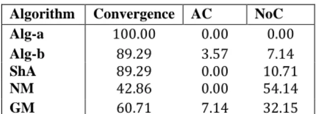
4 Optimization Methods 45 4.1 A Globally Convergent Optimization Algorithm for Systems of Nonlinear Equa-tions . . . 45
4.2 Solving Systems of Nonlinear Equations using a Globally Convergent Opti-mization Algorithm . . . 52
4.3 Globally Convergent Optimization Methods for Unconstrained Problems . . . 60
5 Optimization in Bayesian Networks 76 5.1 Learning Naive Bayes Classifier with Optimization Models . . . 76
5.2 Attribute Weighted Naive Bayes Classifier using a Local Optimization . . . . 88
5.3 Tree Augmented Naive Bayes based on Optimization . . . 103
5.4 Structure Learning of Bayesian Networks using Global Optimization . . . 108
6 Conclusions and Future Work 129 6.1 Summary of Contributions . . . 129
Appendix1 133
Appendix2 134
Bibliography 141
Chapter 1
Introduction
The task of data classification is to assign objects to several predefined categories. Currently, data classification is widely applied in numerous areas, and various techniques have been developed. It is divided to supervised data classification and unsupervised data classifica-tion. This research focuses on Bayesian Networks applied for supervised classifiers involving optimization approaches. Bayesian Networks are among the most commonly used methods in machine learning, and their use have received considerable attention [5, 6, 63, 68].
1.1 Background
The background of this research is presented in two subsections: Bayesian Networks and optimization.
1.1.1 Bayesian Networks
Bayesian Networks are also known as belief networks, causal probabilistic networks, and graphical probability networks. These networks have attracted much attention recently as a possible solution to complex problems related to decision support under uncertainty.
Let us first give a brief discerption to the conditional probability and the Bayes’ Theorem as they are fundamental components of BNs. The probability of event A (an hypothesis)
conditional on the occurrence of some event B (evidence) is denoted by P(A|B). If we are counting sample points, we are interested in the fraction of events B for which A is also true, and we have
P(A|B) = P(A, B) P(B) , this is often written in the form
P(A, B) =P(A|B)P(B),
and referred to as the product rule, this is in fact the simple form of the Bayes Theorem. It is important to realize that this form of the rule is not, as often stated, a definition. Rather, it is a theorem derivable from simpler assumptions. The Bayesian Theorem can be used to tell us how to obtain a posterior probability of a hypothesis A after observation of some evidence B, given the prior probability of A and the likelihood of observing B were A to be the case:
P(A|B) = P(B|A)P(A)
P(B) . (1.1)
Bayesian Networks (BNs) are directed acyclic graphical representations of probabilistic and conditional probabilistic relationships that are constructed by the set of variables. BNs are very successful in reasoning between the variables via conditional probabilities, and have long been used to encode expert knowledge about uncertain domains [54]. To augment available expert knowledge, many researches have been done to construct BNs. Constructing a BN from data is the learning process that is divided in two steps: structure learning and parameter learning. The structure learning process needs to select the arcs (edges) between variables (features) which connect child variables with the set of parent variables, and therefore construct a network from data. In addition to providing a network that will allow us to predict behavior under conditions that we have not seen, the structure can also incorporate
domain expert knowledge to provide more reliable suggestions. Once the structure has been specified, then training the network is straightforward. It consists of computing probabilities and conditional probabilities called parameter learning. Given a set of variables, the more challenging problem is to learn a structure to present the connections among the feature variables.
The learning components of BNs, all together, define the joint probability distribution P(X) for the set of variables X={X1, X2, ..., Xn}, whereXi denotes both the variable and
its corresponding node. Let P a(Xi) denote the set of parents of the node Xi. When there
is an arc from Xi toXj, then Xj is called the child variable for the parent variable Xi. A
conditional dependencyP(Xi|P a(Xi)) connects a child variable with a set of parent variables.
In particular, given a structure, the joint probability distribution forXis given by
P(X) =
n
Y
i=1
P(Xi|P a(Xi))
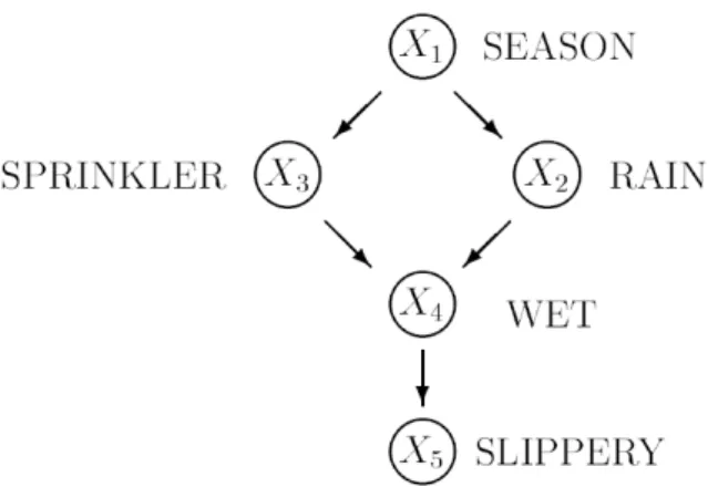
Figure 1.1 illustrates a simple typical BN. It describes the causal relationships among the season of the year (X1), whether rain falls (X2) during the season, whether the sprinkler
is on (X3) during that season, whether the pavement would get wet (X4), and whether the
pavement would be slippery (X5). The joint probability distribution for this sample is:
P(X1, X2, X3, X4, X5) =P(X1)P(X2|X1)P(X3|X1)P(X4|X2, X3)P(X5|X4).
1.1.2 Optimization Problems
Finding parameters and structures in BNs leads to optimization problems. To solve these problems in this thesis, we apply local and global optimization methods. We introduce new globally convergent local optimization methods. The idea in these methods is based on the combination of the gradient and Newton methods. It is well known that the Newton methods have a quadratic convergence rate. However, they are very sensitive to initial points which
Figure 1.1: A Simple Bayesian Network
often lead to failure in practical applications. On the other hand, the gradient methods are globally convergent but they have a linear convergence rate. The proposed methods in this thesis are globally convergent and, at the same time, have high convergence rates. As a global optimization method, we apply the AGOP method introduced in [86, 87]. This algorithm was designed for optimization problems with box constraints. It uses a line search mechanism where the descent direction is obtained via a dynamic systems approach. It is applicable to a wide range of optimization problems requiring only function evaluations to work. We apply this global optimization method in conjunction with the newly suggested local optimization methods.
1.2 Motivation for the Research
The reasons for our choice of BNs are multiple: Firstly, they can encode dependencies among all variables; therefore they readily handle situations where some data entries are missing. BNs are also used to learn causal relationships, and hence can be applied to gain understand-ing about a problem domain and to predict the consequences of intervention. Moreover, since BNs in conjunction with Bayesian statistical techniques have both causal and probabilistic semantics, they are an ideal representation for combining prior knowledge and data. In
dition, BNs in conjunction with Bayesian statistical methods offer an efficient and principal approach for avoiding the over fitting of data [92].
There are several difficulties when applying BNs, which are mainly related to learning pro-cess. Learning parameter with a given structure is one difficulty, whereas learning structure, itself, is another problem. The structural BN learning is much harder problem compared to parameter learning since the number of candidate networks grows exponentially when the number of variables increases. In fact, it has been proved that learning an optimal BN is an NP-hard problem [27, 55]. However, research in this direction is essential because of its enormous usefulness, as much for end user applications.
1.3 Outline of the Thesis
This thesis focuses on BN models; in particular structure learning and parameter learning. We find structures and parameters in BNs by introducing different strategies. Since the definition of structures in BNs is a very difficult problem, priori or manually defined structures are commonly used models for BNs. Naive Bayes (NB) [75] is the most commonly used model of BNs due to its simple structure, fast learning and at the same time being able to provide quite high accuracy in many data classification problems. However, the strong assumption in the NB that all features are conditionally independent given the class is often violated in many real world applications. In this research, we introduce different methods in order to improve the performance of the NB. The first one is alleviating the feature independence assumption. We propose two new algorithms to eliminate this assumption. In the first algorithm, each feature depends on the class and at most one other feature. The dependency between features in this algorithm is found by using conditional probabilities. The second algorithm finds unrestricted dependencies between features iteratively. Each feature in this algorithm has the class and several features as parents. Some features could have a large number of parents, whereas others just have a few. The number of these parents is defined
Another alternative without violating the feature independence assumption in the NB is using feature (attribute) weights. We present a novel attribute weighted NB by assigning weights to conditional probabilities. An objective function has been constructed based on the NB structure and the attribute weights. The number of weights for each attribute is considered as the number of class labels. These weights are considered in the form of powers to conditional attribute class probabilities. The weights, then, are found by using a local optimization method.
We also propose a new algorithm to find an optimal structure in BNs based on global optimization. Although a BN can represent arbitrary feature dependencies, learning an optimal BN from data is an NP-hard problem. To discover better structure, the application of global optimization methods is natural. We apply global optimization method in conjunction with the proposed local methods to find an optimal structure in a BN.
Once the best structure has been specified, then the network is trained by learning pa-rameters. In this research, we introduce three different optimization models to find optimal values of the NB’s parameters. We construct different objective functions with some unknown variables corresponding to class probabilities and conditional feature class probabilities. To optimize these functions to find optimal solutions, we apply newly developed local optimiza-tion methods.
Tree Augmented Naive Bayes (TAN) is another important model in BNs. Unlike the NB, the TAN [42] allows additional edges between features that capture correlations among them. In fact each feature has the class and at most one other feature as parents. Friedman et al. [42], showed that the TAN maintains the robustness of the NB, and at the same time displays better accuracy. The TAN approximates the dependency between features by using a tree structure imposed on the NB structure. In this research, we apply a similar strategy to the NB’s for learning parameters of the TAN. We consider an objective function involving the unknown variables for the class probabilities, and the optimal values of these variables are
computed by applying the proposed local optimization method.
Finally, we introduce our novel local optimization algorithms to solve the models proposed for BNs efficiently. The proposed algorithms are based on the combination of the gradient and Newton based methods. Two different strategies are introduced in this research; in the first one, the step length is determined only along the anti-gradient direction, and in the second case the step length is considered along both directions.
Therefore, the following significant problems are formulated in this thesis:
1. To learn optimal structures in BNs by applying different strategies including optimization techniques.
2. To learn parameters in BNs; in particular the Naive Bayes and the Tree Augmented Naive Bayes, by using optimization formulation for finding the parameters of these models.
3. To develop new optimization methods to solve the optimization problems in 1 and 2 efficiently:
- Local methods: We mainly concentrate on the combination of the gradient method with the Newton
based methods [88, 121, 122].
- Global methods: We apply the method AGOP introduced in [86, 87] in conjunction with the newly suggested local optimization methods.
4. Application of the developed models to the real world problems. We validate the proposed algorithms for BNs using real world data sets taken from the UCI machine learning repository and the LIBSVM.
1.4 Structure of the Thesis
In this section a brief description of the format of the presented thesis (PhD by publication) is given. An introduction is followed by explication of nine papers having different status of publication. A literature review of BNs, local and global optimization methods and
the original formats of published, or submitted to publish of our research work related to BNs, optimization and application of optimization in BNs. The semantic structure for Chap-ters 3 to 5 with the links between the corresponding papers is shown on the next page in a flow chart. In Chapter 3, we introduce new algorithms for learning BNs. In Chapter 4, we propose new local optimization algorithms for solving systems of nonlinear equations and unconstrained optimization problems. Chapter 5 presents applications of the optimization in BNs. We conclude the thesis by providing final remarks and recommendation for future work.
Chapter 2
Literature Review
In this chapter, we present a literature review of Bayesian Networks as well as other concepts and methods related to them which we require for our discussion in the latter part of the Thesis. After a brief description of data classification in Section 2.1, we describe Bayesian Network models in Section 2.2. Subsection 2.2.1 presents approaches to structure learning of Bayesian Network models. In Subsection 2.2.2, we discuss learning the parameters of Bayesian Networks once the structure is known. Some commonly used Bayesian Network models are explained in Subsection 2.2.3 to Subsection 2.2.5. We present several advantages of Bayesian Networks over alternative methods and also applications of them in Subsections 2.2.6 and 2.2.7, respectively. In Section 2.3, we review briefly optimization methods and application of them to Bayesian Networks. Finally, in Section 2.4, we conduct a brief review of discretization methods which we apply in our experiments.
2.1 Data Classification
Data classification is divided into two types: supervised data classification where labeled objects as training sets are required to build the classifier, and unsupervised data classification (clustering), where unlabeled data are fed to the learning system which then chooses an internal organization on its own. The main distinguish between them is that supervised data
classification require a list of predefined classes at the beginning, while unsupervised data classification is given only unlabeled examples. Throughout this research we assume the supervised data classification.
The task of supervised data classification is to assign objects to several predefined cate-gories. For instance, documents can be categorized according to their contents. Examples of classification applications include image and pattern recognition, medical diagnosis, loan approval, detecting faults in industry applications, and classifying financial market trends. Estimation and prediction maybe viewed as types of classification.
According to the number of classes, labels, of a classification problem, there are three main classification categories [80].
1. Binary classification: In this category, there are two classes, such as Yes or No. All examples in this setting will be assigned a positive (1) or negative (−1) integer based on whether or not they belong to the corresponding class.
2. Multi-class classification: In the real world, examples generally have different topics or belong to different classes based on their content. As multi-class setting attempts to classify examples based on their main topic, so that examples can belong to one and only one class. In order to deal with multi-class problems, different approaches have been ex-plored in the literature. There are two types of approaches for multi-class classification. The first one is constructing and combining several binary classifiers, called decomposition ap-proaches. Another one is considering all data in one optimization formulation, called single machine approaches. Several methods have been proposed for decomposition approaches, for instance, one-vs-all approaches [9, 106], all-vs-all approaches [42, 50], and error-correcting code approaches [2, 29, 32]. Unlike the decomposition approaches, the single machine ap-proach attempts to solve a single optimization problem to find q functions simultaneously rather than combine the solutions to a collection of binary problems [129] and [132].
3. Multi-label classification: If an example can belong to more than one class, then we have a set of multi-labeled classification problems. There exists a number of multi-label
multi-label classification methods into two main categories: problem transformation methods and algorithm adaptation methods [80].
2.2 Bayesian Networks
Bayesian Networks (BNs) are high level representations of probability distributions over a set of variables that are used for building a model of the problem domain. The benefit of BNs lies in the way such a model (structure) can be used as a compact representation for many naturally occurring and complex problem domains.
BNs were developed in the late 1970’s to model the semantic and perceptual combination of evidence in reading. The capability for bidirectional inferences, combined with a rigorous probabilistic foundation, led to the rapid emergence of BNs at the early 1980’s as the method of choice for uncertain reasoning in artificial intelligence, expert system, statistic and data mining [24, 53, 61, 100, 113]. For an introductory overview of BNs, we refer the reader to [25, 61, 100] and for a detailed analysis, to [53, 62, 101].
A BN is associated with a directed acyclic graph. The nodes in the graph correspond to the feature variables in the domain, and the arcs (edges) show the causal relationships between feature variables. The direction of the arrow indicates the direction of causality. Edges also determine some qualifying terms for nodes. When two nodes are joined by an edge, the causal node is called the parent of the other node, and another one is called the child. Other terminology you might encounter includes the term root node for any node without parents and leaf node for any node without children. Therefore, a graph G = (V, E) is simply a collection of variablesV and edges E between variables.
How one node influences another is defined by the conditional probabilities for the nodes, that describes the relationship between it and its parents. Conditional probabilities represent likelihoods based on prior information or past experience. For each parent and each possible
state of that parent, there is a row in the conditional probability table (CPT) that describes the likelihood that the child node will be in some state. Nodes with no parents also have CPTs, but they are simpler and consist only of the probabilities for each state of the node under consideration.
A BN for a set of variables X = {X1, X2, ..., Xn} consist of a network structure B that
encodes a set of conditional dependencies assertions about variables in X, and a set P of local probability distributions associated with each variable. Together, these components define the joint probability distribution forX. The network structureB is constrained to be acyclic. The nodes inB are in one to one correspondence with the variableX. We useXi to
denote both the variable and its corresponding node. Let P a(Xi) denote the set of parents
of the nodeXi inX as well as variables corresponding to those parents. The lack of possible
arcs inB encode conditional independencies. In particular, given the structure B, the joint probability distribution for Xis given by
P(X) =
n
Y
i=1
P(Xi|P a(Xi)). (2.1)
In the light of the above information, properties of BNs can be summarized as below [109]: 1. It has a set of variables and a set of directed edges between variables.
2. Each variable contains a finite set of mutually exclusive states.
3. The variables coupled with the directed edges construct a directed acyclic graph (DAG). 4. Each variableXi, 1 ≤i≤n, with its parents has a conditional probability table (CPT)
associated with it.
5. It has a joint probability distribution forX={X1, X2, ..., Xn}, given by formula (2.1).
If variableXi, 1≤i≤n,does not have any parents, then the conditional probability table
can be replaced by the probability P(Xi). A graph is acyclic if there is no directed path X1 →X2...→Xn such thatX1=Xn.
Most of BNs researches can be put into two main categories. First, given a BN model
a set of observed variables. This process is referred to as BN inference [62]. Second, given a collection of data, what is the most appropriate BNs model that describes it. In this research we concentrate on the second category. BNs model identification can be separated into two tasks: structure learning and parameter learning. Structure learning is related to a graph and not to the values of the probabilities. Given a structure, parameter learning is related to find probabilities and conditional probabilities among variables.
There are four classes of learning BNs from data: 1. Known structure and complete data
In this case, the problem is to calculate the conditional probability tables of each node in the network from the complete data (parameter learning). This is a relatively easier problem and has been studied extensively [117].
2. Known structure and incomplete data
The problem of learning parameters for a fixed network in the presence of missing values or hidden variables studied by extending and adapting expectation-maximization (EM) al-gorithm [43] and by Gibbs sampling. Both of these alal-gorithms use a basic strategy that is to estimate the missing data on the basis of available data and information about the missing data. Another approach, called bound and collapse (BC) [110], first bounds the set of possible estimates consistent with the available information by computing the optima of estimates that are gathered from all possible completions of the database constraint by the given pattern of the missing data and then collapses these bounds to a point estimate using information about the assumed pattern of missing data. Genetic algorithm [91] is used to evolve both the missing values and the structures to find an optimal BN.
3. Unknown structure and complete data
Our problem falls into this category in which we are given a complete data set and asked to generate the structure of BNs that fits the data the best.
4. Unknown structure and incomplete data
Since it is generally not feasible to compute exact solutions to this problem, approximate al-gorithms generally employed. It is first attacked by a gradient-based algorithm [107] by using structural EM (SEM) that optimizes parameters with structure search for model selection. Convergence to a sub-optimal network and need for heavy computation during the learning are major problems with the structural SEM algorithm. Another approach is to use above mentioned BC for incomplete data [110]. The problem of learning an optimal structure of a BN from incomplete data is also considered in [134].
The problem we attack falls into the third class in which we try to learn the structure of BNs by using the observed data.
2.2.1 Structure Learning
Structure learning is the task of finding out one graph model that best characterizes the true density of given data. Perhaps the most challenging task in dealing with a BN is learning the structure. However, research in this direction is essential because of its enormous usefulness, as much for end-user applications.
Structure learning can be categorized into two levels: micro-level (quantitative part) and macro-level (qualitative part). In the micro-level, structure learning cares about whether one edge in the graph should be existed or not. In this case, researchers usually employ the conditional independence test to determine the importance of edges [26, 101, 118]. In the macro-level, several candidate graph structures are known, and we need choosing the best one out. In order to avoid over fitting, model selection methods, such as Bayesian scoring function [28, 52], entropy-based method [56], and minimum descriptive length (MDL), etc [22, 42] are often used. Therefore, learning structure of BNs can be divided in two main categories:
1. Constraint-based Methods: Finding dependencies between the random variables; some well known algorithms are IC [101], PC [118], and recently TPDA of Cheng et al. [26]. 2. Score-based Methods: Using heuristic searching methods to construct a model and then
Bayesian Information Criteria (BIC) [112], Normalized Minimum Likelihood (NML) [72– 74], Mutual Information Tests (MIT) [21, 126] and Minimum Description Length (MDL) principal [22, 42], Bayesian Dirichlet (BD) score [28], Bayesian Dirichlet equivalence (BDE) [53], Bayesian Dirichlet equivalence uniform (BDEU) [14], BDgamma [12], CCL [48] and ACL [16].
Both of these categories have their advantage and disadvantage. Generally the first one is asymptotically correct when the probability distribution of data satisfies certain assumption, but as Cooper et al. pointed out in [56], conditional independency tests with large condition sets may be unreliable. The second one has less time complexity in the worst case, but it may not find the best solution due to its heuristic nature.
2.2.2 Parameter Learning
Given a structure, learning the parameters are related to finding probabilities and conditional probabilities. There are two approaches of parameter learning: generative and discrimina-tive. In generative parameter learning, a model of joint probability of the features and corresponding class label are learnt and then prediction is performed by using the Bayes’ rule to determine the class posterior probability. Maximum likelihood (ML) estimation is usually used to learn a generative classifier. Discriminative approaches model the class posterior probability directly. Hence, the class conditional probability is optimized when we learn the classifier which is the most important for classification accuracy.
There are some methods for finding parameters such as ML, ECL, ACL, and CGCL pa-rameter learning [102]. Learning papa-rameters from data, in detail, is discussed in [15, 116] and [11, 46, 125].
Some well known BN models are Naive Bayes [36, 75], Tree Augmented Naive Bayes [42], Super Parent BNs [69], andk-dependence BN [108] which will be presented in the following.
2.2.3 Naive Bayes Classifier
Naive Bayes classifier [75] has the simplest structure among BN models. It assumes that all features are conditionally independent given the class; it means that all features have only the class as a parent. The Naive Bayes (NB) is attractive as it has an explicit and sound theoretical basis which guarantees optimal induction given a set of explicit assumptions. There is a drawback, however, in that some of these assumptions will be violated in many induction scenarios. In particular, one key assumption that is frequently violated is that the features are independent with respect to the class. The NB has been shown to be remarkably robust in the face of many such violations of its underlying assumptions [33].
Let us denote the class of an observationXbyC, whereC ∈ {C1,· · · , Cq}. To predict the
class of a test observationX by using Bayes’ rule, the highest probability of
P(C=c|X=x) = P(C=c)P(X=x|C=c)
P(X=x) , (2.2)
should be found, wherecrepresents a particular class label andx={x1, x2, ..., xn}stands for
a particular observed feature value. Since in the NB, featuresX1, X2, ..., Xnare conditionally
independent given the classC, the formula (2.2) could be written as
P(C =c|X= x) = P(C=c) Qn
i=1P(Xi =xi|C=c)
P(X=x) . (2.3)
Therefore, the NB classifies an observationX by selecting
arg max 1≤k≤qP(Ck|X)∝arg max1≤k≤mP(Ck) n Y i=1 P(Xi|Ck). (2.4)
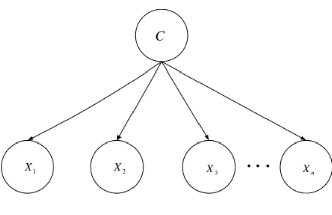
A sample of the NB classifier withnfeatures is depicted in Figure 2.1.
1
X X2 X3 Xn
Figure 2.1: Naive Bayes
2.2.4 Tree Augmented Naive Bayes
Friedman et al. proposed Tree Augmented Naive Bayes (TAN) [42]. The TAN attempts to add edges to the NB. In fact each feature has the class and at most one other feature as parents. The TAN approximates the dependency between features by using a tree structure imposed on the NB structure. They showed that the TAN maintains the robustness and com-putational complexity of the NB, and at the same time displays better accuracy. Algorithm TAN consists of five main steps:
Algorithm. Tree Augmented Naive Bayes Algorithm
Step 1. Compute the conditional mutual information I(Xi;Xj|C) for each pair of features i6=j, using (2.6).
Step 2. Build a complete undirected graph in which the vertices are the featuresX1, ..., Xn.
Annotate the weight of an edge connectingXi toXj by I(Xi;Xj|C).
Step 3. Build a maximum weighted spanning tree.
Step 4. Transform the resulting undirected tree to a directed one by choosing a root variable and setting the direction of all edges to be outward from it.
Step 5. Construct the TAN model by adding a vertex labled by C and adding an arc from C to each Xi.
This procedure reduces the problem of constructing a maximum likelihood tree to finding a maximal weighted spanning tree in a graph. The problem of finding such a tree is to select a subset of arcs from a graph such that the selected arcs constitute a tree and the sum of weights attached to the selected arcs is maximized.
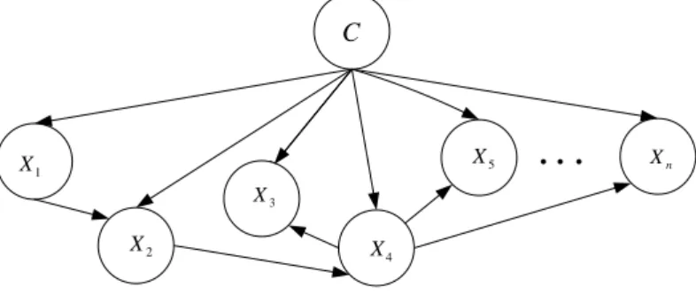
The directions of edges in the TAN are crucial. In Step 4 of the TAN algorithm, a feature is randomly chosen as the root of the tree and the directions of all edges are set outward from it. Notice that the selection of the root feature actually determines the structure of the resulting TAN. Figure 2.2 shows a sample of the TAN withnfeatures.
C 2 X 4 X 1 X 3 X 2 X 3 X 4 X 5 X Xn C
Figure 2.2: Tree Augmented Naive Bayes
In information theory, the mutual information of two nodesXi, Xj is defined as
I(Xi;Xj) = X xi∈Xi,xj∈Xj P(xi, xj)log P(xi, xj) P(xi)P(xj) (2.5)
and the conditional mutual information is defined as
I(Xi;Xj|C) = X xi∈Xi,xj∈Xj,c∈C P(xi, xj, c)log P(c)P(xi, xj, c) P(xi, c)P(xj, c) . (2.6) 19
In this subsection, we present an algorithm [108] which allows us to construct classifiers at arbitrary points (values ofk) along the feature dependence, while also capturing much of the computational efficiency of the NB.
Thek-dependence BN allows each featureXi to have a maximum ofkfeatures as parents,
i.e., the number of variables in P a(Xi) equals to k+ 1; k features and 1 class. In the k
-dependence BN, the number k is a priori chosen. According to the definition, the NB is a 0-dependence BN.
Algorithm. k-dependency Algorithm
Step 1. For each featureXi, compute mutual informationI(Xi;C), using (2.5), whereC is
the class.
Step 2. Compute class conditional mutual information I(Xi;Xj|C), using (2.6), for each
pair of featuresXi andXj, where i6=j.
Step 3. Let the used variable list, S, be empty.
Step 4. Let the BN being constructed begin with a single class node, C. Step 5. Repeat until S includes all domain features:
5.1. Select featureXmax, which is not inS and has the largest value I(Xmax;C).
5.2. Add a node to the BN representingXmax.
5.3. Add an arc fromC toXmax in BN.
5.4. Add m=min(|S|, k) arcs from m distinct features Xj in S with the highest value for I(Xmax;Xj|C).
5.5. Add Xmax toS.
Step 6. Compute the conditional probability tables inferred by the structure of the BN.
2.2.6 Advantages of Bayesian Networks
BNs offer several advantages over alternative modeling approaches [54]. The most important of these advantages are:
1. BNs encode dependencies among all variables, therefore, they readily handle situations where some data entries are missing.
For example, consider a classification or regression problem where two of the variables are strongly anti correlated. This correlation is not a problem for standard supervised learning, provided all inputs are measured in every case. When one of the inputs is not observed, however, many models will produce an inaccurate prediction, because they do not encode the correlation between the variables. BNs offer a natural way to encode such dependencies.
2. BNs can be used to learn causal relationships, and hence, can be used to gain under-standing about a problem domain and to predict the consequences of intervention.
Learning about causal relationships are important for at least two reasons. The process is useful when we are trying to gain understanding about a problem domain, for example, during exploratory data analysis. In addition, knowledge of causal relationships allows us to make predictions in the presence of interventions. For example, a marketing analyst may want to know weather or not it is worthwhile to increase exposure of a particular advertisement in order to increase the sales of product. To answer this question, the analyst can determine whether or not the advertisement is a cause for increased sales, and to what degree. The use of BNs helps to answer such questions even no experiment about the effects of the increased exposure is available.
3. Because BNs in conjunction with Bayesian statistical techniques have both causal and probabilistic semantics, they are an ideal representation for combining prior knowledge (which often comes in causal form) and data.
Anyone who has performed a real world modeling task knows the importance of prior or domain knowledge, especially when data is scarce or expensive. The fact that some
knowledge. BNs have a causal semantics that makes the encoding of causal prior knowledge particularly straightforward. In addition, BNs encode the strength of causal relationships with probabilities.
4. BNs in conjunction with Bayesian statistical methods offer an efficient and principal approach for avoiding the over fitting of data.
2.2.7 Applications of Bayesian Networks
BNs have gained wide spread use in data mining [131]. They are offering a compact pre-sentation of the interactions in a stochastic system by visualizing system variables and their dependencies, and therefore, they have been applied in electricity distribution system risk management [98]. BNs are risk modelings and analysis approaches that have been used for various types of analysis for different purposes in industrial sectors [4, 65, 98, 127].
BNs are hand-built by medical experts and later used to infer likelihood of different causes given observed symptoms,therefore, they have been used to build medical diagnostic systems [40]. Similar systems have also been built for diagnosing problems in factories and other mechanical systems [93]. In systems biology, a BN structure learning is used to infer different types of biological networks from data [95].
Burnell and Horvitz [19] show how BNs and logical approaches can be married for program understanding and debugging. Fung and Del Falvero described an application of BNs to information retrieval [44]. Hekerman et al. [51] show how BNs can be used for troubleshooting system failures, including software and hardware problems as well as mechanical failures of cars and jet engines.
With the advent of small, powerful computers and GUI interfaces, modeling tools based on BNs are seeing frequent use in real world applications including diagnosis [3], forecasting [49], automated vision [81], sensor fusion [115], and manufacturing control [135]. BNs are general modeling frameworks which have been extensively applied in business and finance, capital
equipment, causal modeling, natural language processing, planning, psychology, scheduling, speech recognition, vehicle control, forecasting, channel coding, and commonsense reasoning problems [31, 94, 130].
2.3 Optimization in Bayesian Networks
Finding parameters and structures in BNs leads to some optimization problems. In this section, we present a brief review about these optimization problems [8, 13, 97, 120], and then we will give a literature review of optimization methods in BNs.
Optimization is a very important tool in decision science. To use it, we must first identify some objective, a quantitative measure of the performance of the system under study. The objective depends on certain characteristics of the system, called variables or unknowns. The goal is to find values of the variables that optimize the objective. Often the variables are restricted, or constrained, in some way. The process of identifying objective, variables, and constraints for a given problem is known as modeling. Construction of an appropriate model is the first step in the optimization process. If the model is too simplistic, it will not give useful insights into the practical problem, but if it is too complex, it may become too difficult to solve. Methods for solving optimization problems take two different approaches; local optimization and global optimization. In local optimization, the compromise is to give up seeking the optimal point, which minimizes the objective over all feasible points. Instead we seek a point that is only locally optimal, which means that it minimizes the objective function among feasible points that are near it, but is not guaranteed to have a lower objective value than all other feasible points. Local optimization methods are fast, can handle large scale problems, and are widely applicable. However, there are several disadvantages of local optimization methods, beyond (possibly) not finding a globally optimal solution. The methods require an initial guess for variables. This initial guess or starting point is critical, and can greatly affect the objective value of the local solution obtained. To find a global
optimization is usually used for problems with a small number of variables, where computing time is not critical. However, it is worthwhile to use it in cases where the value of finding a global solution is very high, or the cost of being wrong about the reliability or safety is high. Optimization problems could be classified according to the nature of the objective func-tion and constraints (linear, nonlinear, convex), the number of variables (large or small), the smoothness of the functions (smooth or non-smooth), and so on. Some models con-tain variables that are allowed to vary continuously and others that can atcon-tain only integer values; these models are called mixed integer programming problems. Possibly an impor-tant distinction between problems is that have constraints on variables and those that do not. Constrained optimization problems arise directly in many practical applications. Un-constrained problems arise also as reformulations of Un-constrained optimization problems, in which the constraints are replaced by penalization terms in the objective function that have the effect of discouraging constraint violations.
Optimization models constructed for BNs are usually constrained problems. To transform these problems in to unconstrained cases, most of the researchers in this area used the La-grange method [10], [59], [123], [102], [105], [58], [82], [90], [96], [47], [17], while others applied the penalty method [114], [35], [123], [45], [83], [71] and [66].
To solve unconstrained problems, one can use local or global optimization methods. Exist-ing local methods used for optimizExist-ing BNs are gradient-based methods; for instance, Wilson et al.[133], Kitakoshi et al. [70], Jing et al. [63], Burge [16], Bang and Gil [7] applied the Gradient method. Pernkopf and Wohlmayr [102], Hinsbergen et al. [57] and Greiner et al. [47] used the Conjugate Gradient method. Quasi Newton method has been used by Zhang et al. [82].
Recently, researchers were more interested using global search methods for BNs’ optimiza-tion. Various problems to learn a structure of a BN using global optimization have been defined [99], [77], [79], [78], [67], [111], [60], [140], [109], [30], [84], [22], [85]. Park and Cho
[99] used the Genetic algorithm to optimize the structure in BNs and make a model more efficient. A method of finding the most probable structure of BNs based on the intelligent search made by the Genetic algorithm has been introduced by Larranaga et al. [79]. The papers [77], [78], [103], [137], [136], and [37] present several new approaches based on the Genetic algorithm to find the best BNs’ structure among alternative structures. Work by Kabli et al. [67] illustrates a novel method for finding the structure of BNs using the Genetic algorithm. They proposed a method that uses chain structures as a model for BNs that can be constructed from given node orderings. The simulated annealing approaches to learning the structure in BNs have been studied, for example, in [111], [60], [119]. Application of the Particle Swarm optimization to discover the best structure of BNs is studied in [140], [109]. Daly and Shen [30] applied the Ant Colony optimization to the problem of learning BNs’ structure that provides a good fit to data. The papers [84], [20], [30] propose BNs’ structure learning algorithms based on the Ant Colony optimization. Marinescu and Dechter [85] and Cano et al. [23] applied the Branch and Bound method to learn the structure of BNs.
2.4 Discretization of Continuous Features
BNs learning needs to estimate probabilities and conditional probabilities for each class and feature-class from data set. For a qualitative feature, its relevant probabilities can be esti-mated from the corresponding frequencies. For a quantitative feature, its relevant probabil-ities can be estimated if we know the probability distributions from which the quantitative values are drawn. However, those distributions are usually unknown for real world data. Thus how to deal with quantitative features is a key problem in BNs learning. Typically, there are two approaches to tackling this problem.
The first approach is probability density estimation that makes assumptions about the probability density function of a quantitative feature given a class. The relevant probabilities can then be estimated accordingly. For instance, a conventional approach is to assume that
is made because a normal distribution may provide a reasonable approximation to many real world distributions [64], or because the normal distribution is perhaps the most well studied probability distribution in statistics [89].
A second approach is discretization. Under discretization, a qualitative feature is created for a quantitative feature. Each value of the qualitative feature corresponds to an interval of values of the quantitative feature. The resulting qualitative features are used instead of the original quantitative features to train a classifier. Since the probabilities of a qualitative feature can be estimated from its frequencies, it is no longer necessary to assume any form of distributions for the quantitative features.
For BNs learning, discretization is more popular than assuming probability density func-tion. The main reason is that the true density is usually unknown for real world data, and therefore, BN classifiers with discretization tend to achieve lower classification error than those with unsafe probability density assumptions [34].
A typical discretization process broadly consists of four steps: 1. Sorting the continuous values of the feature to be discretized.
2. Evaluating a cut-point for splitting or adjacent intervals for merging.
3. According to some criterion, splitting or merging intervals of continuous value. 4. Finally stopping at some point.
After sorting, the next step in the discretization process is to find the best cut-point to split a range of continuous values or the best pair of adjacent intervals to merge. One typical evaluation function is to determine the correlation of a split or a merge with the class label. A stopping criterion specifies when to stop the discretization process. It is usually governed by a trade-off between lower arty with a better understanding but less accuracy and a higher arty with a poorer understanding but higher accuracy. The number of inconsistencies caused by discretization should not be much higher than the number of inconsistencies of the original data before discretization. Two instances are considered inconsistent if they are the same in
their feature values except for their class labels.
Generally, the discretization methods could be supervised or unsupervised. A distinction can be made dependent on whether the method takes class information into account to find proper intervals or not. The methods that do not make use of class membership informa-tion during the discretizainforma-tion process are referred to as unsupervised methods. In contrast, discretization methods that use class labels for carrying out discretization are referred to as supervised methods. There are several supervised and unsupervised methods to discretize quantitative features [138]. In following subsections, we present the most popular supervised discretization method, Fayyad and Irani’s method, and the newest unsupervised discretiza-tion algorithm, using sub-optimal agglomerative clustering method (SOAC).
2.4.1 Fayyad and Irani’s Discretization Method
In this subsection, we present Fayyad and Irani’s Discretization algorithm [38]. The Fayyad and Irani’s Discretization method is based on a minimal entropy heuristic, and it uses the class information entropy of candidate partitions to select bin boundaries for discretization.
Let us consider a given set of observations S, a feature X, and a partition boundary T, the class information entropy of the partition induced byT, denoted E(X, T;S) is given by
E(X, T;S) = |S1|
|S|Ent(S1) + |S2|
|S|Ent(S2),
where S1 ⊂S be the subset of observations in S with X-values not exceeding T and S2 =
S−S1.Let there be q classesC1, ..., Cq, and P(Ci, S) be the proportion of observations inS
that have classCi . The class entropy of a subset S is defined as:
Ent(S) =− q X i=1 P(Ci, S) lg(P(Ci, S)), 27
the amount of information needed, in bits, to specify the classes inS.
For a given feature X, the boundary Tmin which minimizes the entropy function over all
possible partition boundaries is selected as a binary discretization boundary. This method can then be applied recursively to both of the partitions induced byTminuntil some stopping
condition is achieved, thus creating multiple intervals on the featureX.
Fayyad and Irani make use of the minimal description length principle to determine a stopping criteria for their recursive discretization strategy. Recursive partitioning within a set of values S stops if
Gain(X, T;S)< lg2(N−1)
N +
4(X, T;S)
N ,
whereN is the number of observations in the setS, and
Gain(X, T;S) =Ent(S)−E(X, T;S),
4(X, T;S) = lg2(3q−2)−[q.Ent(s)−q1.Ent(S1)−q2Ent(S2)],
andqi is the number of class labels represented in the setSi. Since the partitions along each
branch of the recursive discretization are evaluated independently using this criteria, some areas in the continuous spaces will be partitioned very finely whereas others (which have relatively low entropy) will be partitioned coarsely.
2.4.2 Discretization Algorithm using Sub-Optimal Agglomerative Clustering
In this section, we present the discretization algorithm using sub-optimal agglomerative clus-tering (SOAC) [139]. Let us consider a finite set of points A in the n−dimensional space
Rn, that is A ={a1, ..., am}, where ai ∈Rn, i= 1, ..., m. Assume the sets Aj, j = 1, ..., k be clusters, and each clusterAj can be identified by its centroid xj ∈Rn, j = 1, ..., k.The Algorithm SOAC proceeds as follows.
Algorithm. Discretization Algorithm SOAC
Step 1. Set k=m,and a small value of parameterθ, 0< θ <1. Sort values of the current feature in the ascending order. Each continuous feature requiring discretization is treated in turn.
Step 2. Calculate the center of each cluster:
xj = X
a∈Aj a
|Aj|, j = 1, ..., k
and the errorEk of the cluster system approximating set A:
Ek = k X j=1 X a∈Aj kxj−ak2.
Step 3. Merge in turn each cluster with the next tentatively. Calculate the error increase Ek−1−Ek after each merge and choose the pair of clusters giving the least increase. Merge
these two clusters permanently. Setk=k−1.
Step 4. If Ek≥θE1,then stop, otherwise go to Step 2.
Chapter 3
Bayesian Networks
3.1 Improving Naive Bayes Classifier using Conditional
Probabilities
This section is devoted to a new algorithm for improving Naive Bayes classifier. The Naive Bayes classifier is the simplest among Bayesian Networks, and it performs very well on a variety of data classification problems. However, the strong assumption that all features are conditionally independent given the class is often violated in many real world applications. The proposed algorithm, in this section, finds dependencies between features using conditional probabilities. The performance of the algorithm is empirically validated using real world data sets. The experimental results demonstrate that the proposed algorithm significantly improve the performance of the Naive Bayes classifier, yet at the same time maintains its robustness.
Paper:
Improving Naive Bayes Classifier using Conditional Probabilities
Published by:
9-th Australasian Data Mining Conference, Ballarat, Australia, Volume 121, pp. 63-68, 2011
Authors: Sona Taheria, Musa Mammadova, b and Adil M.Bagirova
aCentre for Informatics and Applied Optimization,
School of Science, Information Technology and Engineering, University of Ballarat, VIC 3353, Australia
bNational ICT Australia, VRL, VIC 3010, Australia
Corresponding author: Sona Taheri
e-mail: [email protected]
Improving Naive Bayes Classifier
Using Conditional Probabilities
SONA TAHERI1 MUSA MAMMADOV1,2 ADIL M. BAGIROV1
1Centre for Informatics and Applied Optimization, School of Science, Information Technology and
Engineering, University of Ballarat, Victoria 3353, Australia
2 National Information and Communications Technology Australia (NICTA)
Emails: [email protected], [email protected], [email protected]
Abstract
Naive Bayes classifier is the simplest among Bayesian Network classifiers. It has shown to be very efficient on a variety of data classification problems. However, the strong assumption that all features are condition-ally independent given the class is often violated on many real world applications. Therefore, improve-ment of the Naive Bayes classifier by alleviating the feature independence assumption has attracted much attention. In this paper, we develop a new version of the Naive Bayes classifier without assuming inde-pendence of features. The proposed algorithm ap-proximates the interactions between features by using conditional probabilities. We present results of nu-merical experiments on several real world data sets, where continuous features are discretized by apply-ing two different methods. These results demonstrate that the proposed algorithm significantly improve the performance of the Naive Bayes classifier, yet at the same time maintains its robustness.
Keywords: Bayesian Networks, Naive Bayes, Semi Naive Bayes, Correlation
1 Introduction
Classification is the task to identify the class labels for instances based on a set of features, that is, a function that assigns a class label to instances de-scribed by a set of features. Learning accurate clas-sifiers from pre classified data is an important re-search topic in machine learning and data mining. One of the most effective classifiers is Bayesian Net-works (Shafer 1990, Heckerman 1995, Jensen 1996, Pearl 1996, Castillo 1997). A Bayesian Network (BN) is composed of a network structure and its conditional probabilities. The structure is a directed acyclic graph where the nodes correspond to domain vari-ables and the arcs between nodes represent direct de-pendencies between the variables. Considering an in-stance X = (X1, X2, ..., Xn) and a class C, the clas-sifier represented by BN is defined as
arg max c∈C P(c|x1, x2, ..., xn)∝arg max c∈C P(c)P(x1, x2, ..., xn|c), (1)
where xi, care the values ofXi, C respectively.
Copyright c�2011, Australian Computer Society, Inc. This pa-per appeared at the 9th Australasian Data Mining Conference (AusDM 2011), Ballarat, Australia, December 2011. Confer-ences in Research and Practice in Information Technology (CR-PIT), Vol. 121, Peter Vamplew, Andrew Stranieri, Kok-Leong Ong, Peter Christen and Paul Kennedy, Ed. Reproduction for academic, not-for-profit purposes permitted provided this text is included.
However, accurate estimation ofP(x1, x2, ..., xn|c) is non trivial. It has been proved that learning an op-timal BN is NP-hard problem (Chickering 1996, Heck-erman 2004). In order to avoid the intractable com-plexity for learning BN, the Naive Bayes classifier has been used. In the Naive Bayes (NB) (Langley 1992, Domingos 1997), features are conditionally indepen-dent given the class. The simplicity of the NB has led to its wide use, and to many attempts to extend it (Domingos 1997). Since NB assumes the strong assumption of independency between features, learn-ing semi Naive Bayes has attracted much attention from researchers (Langley 1994, Kohavi 1996, Paz-zani 1996, Friedman 1997, Kittler 1986, Zheng 2000, Webb 2005). The semi Naive Bayes classifiers are based on the structure of NB, requiring that the class variable be a parent of every feature. However, they allow additional edges between features that capture correlation among them. The main aim in this area of research has involved maximizing the accuracy of classifier predictions.
In this paper, we propose a new version of the Naive Bayes classifier (semi Naive Bayes) without as-suming independence of features. The proposed algo-rithm finds dependencies between features using con-ditional probabilities. This algorithm is a new al-gorithm and different from the existing semi Naive Bayes methods (Langley 1994, Kohavi 1996, Pazzani 1996, Friedman 1997, Kittler 1986, Zheng 2000, Webb 2005).
Most of data sets in real world applications often involve continuous features. Therefore, continuous features are usually discretized (Lu 2006, Wang 2009, Ying 2009, Yatsko 2010). The main reason is that the classification with discretization tend to achieve lower error than the original one (Dougherty 1995). We apply two different methods to discretize continu-ous features. The first one, which is also the simplest one, transforms the values of features to{0,1} using their mean values. We also apply the discretization algorithm using sub-optimal agglomerative clustering algorithm from (Yatsko 2010) which allows us to get more than two values for discretized features. This leads to the design of a classifier with higher testing accuracy in most data sets used in this paper.
We organize the rest of the paper as follows. We give a brief review to the Naive Bayes and some semi Naive Bayes classifiers in Section 2. In Section 3, we present the proposed algorithm. Section 4 presents an overview of the discretization algorithm using sub-optimal agglomerative clustering. The numerical ex-periments are given in Section 5. Section 6 concludes the paper.
2 Naive Bayes and Semi Naive Bayes Classi-fiers
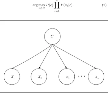
The Naive Bayes (NB) assumes that the features are independent given the class, it means that all features have only the class as a parent (Kononenko 1990, Lan-gley 1992, Domingos 1997, Mitchell 1997). A sample of the NB withnfeatures is depicted in Figure 1. The NB, classifies an instanceX = (X1, X2, ..., Xn) using Bayes rule, by selecting
arg max c∈C P(c) n � i=1 P(xi|c). (2) C 1 X X2 X3 xx x Xn
Figure 1: Naive Bayes
NB has been used as an effective classifier for many years. Unlike many other classifiers, it is easy to con-struct, as the structure is given a priori. Although the independence assumption is obviously problem-atic, NB has surprisingly outperformed many sophis-ticated classifiers, especially where the features are not strongly correlated (Domingos 1997). In spite of NB’s simplicity, the strong independency assumption harms the classification performance of NB when it is violated. On the other hand, learning BN requires searching the space of all possible combinations of edges which is NP-hard problem (Chickering 1996, Heckerman 2004).
In order to relax the independence assumption of NB, a lot of effort has focussed on improving NB. The improved NB classifiers use exhaustive search to join features based on statistical methods. There are some improved algorithms of the NB. Langley and Sage (Langley 1994) considered Backwards Sequen-tial Elimination (BSE) and Forward SequenSequen-tial Se-lection (FSS) in which their methods select a subset of features using leave-one-out cross validation error as a selection criterion and establish a NB with these features. Starting from the full set of features, BSE successively eliminates the features whose elimination most improves accuracy, until there is no further ac-curacy improvement. FSS uses the reverse search di-rection, that is iteratively adding the features whose addition most improves accuracy, starting with the empty set of features. The work of Pazzani (Paz-zani 1996) introduces Backward Sequential Elimina-tion and Joining (BSEJ). It uses predictive accuracy as a merging criterion to create new Cartesian prod-uct features. The value set of a new compound fea-tures is the Cartesian product of the value sets of the two original features. As well as joining features, BSEJ also considers deleting features. BSEJ repeat-edly joins the pair of features or deletes the features
that most improves predictive accuracy using leave-one-out cross validation. This process terminates if there is no accuracy improvement. Kohavi (Kohavi 1996) proposed the NB Tree, a strategy that is a hy-brid approach combining NB and decision tree learn-ing. It partitions the training data using a tree struc-ture and establishes a local NB in each leaf. It uses 5-fold cross validation accuracy estimate as the split-ting criterion. A split is defined to be significant if the relative error reduction is greater than 5 percent and the splitting node has at least 30 instances. When there is no significant improvement, NB Tree stops the growth of the tree. As the number of splitting features is greater than or equals one, NB Tree is an x-dependence classifier. The classical decision tree predicts the same class for all the instances that reach a leaf. In NB Tree, these instances are classified us-ing a local NB in the leaf, which only considers those non tested features. Friedman et al. (Friedman 1997) introduced Tree Augment Naive Bayes (TAN) based on tree structure. It approximates the interactions between features by using a tree structure imposed on the NB structure. In TAN, each feature has the class and at most one other feature as parents. Super Parent algorithm is proposed by Keogh and Pazzani (Keogh 1999). This algorithm uses the same represen-tation as the Tree Augment Naive Bayes, but utilizes leave-one-out cross validation error as a criterion to add a link. The Super Parent is the feature that is the parent of all the other orphans, the features with-out a non-class parent. There are two steps to add a link: first selecting the best Super Parent that im-proves accuracy the most, and then selecting the best child of the Super Parent from orphans. This method stops adding links when there is no accuracy improve-ment. Zheng and Webb (Zheng 2000) developed Lazy Bayesian Rules (LBR), which adopts a lazy approach, and generates a new Bayesian rule for each test exam-ple. The antecedent of a Bayesian rule is a conjunc-tion of feature-value pairs, and the consequent of the rule is a local NB, which uses those features that do not appear in the antecedent to classify. LBR stops adding feature value pairs into the antecedent if the outcome of a one tailed pairwise sign test of error dif-ference is not better than 0.05. As the number of the feature value pairs in the antecedent is greater than or equals one, LBR is anx-dependence classifier. Webb et al. (Webb 2005) proposed Averaged One Depen-dence Estimators (AODE), which averages the pre-dictions of all qualified 1-dependence classifiers. In each 1-dependence classifier, all features depend on the class and a single feature.
In the next section, we introduce a new version of the Naive Bayes classifier (semi Naive Bayes) with-out assuming independence of features. The proposed algorithm approximates the interactions between fea-tures by using conditional probabilities.
3 The Proposed Algorithm
In this section, we present a new algorithm that main-tains the basic structure of the NB, and thus ensure that the class C is the parent of all features. The proposed algorithm, however, removes the strong as-sumption of independence in the NB by finding corre-lation between features, while also capturing much of the computational efficiency of the NB. In this algo-rithm, the class has no parents and each feature has the class and at most one other feature as parents. Therefore, each feature can have one augmenting edge pointing to it. The procedure for learning these edges is based on the Pearson’s correlation and conditional CRPIT Volume 121 - Data Mining and Analytics 2011
probabilities. First, we construct a basic structure of the NB with n features X1, X2, ..., Xn from the set
X and the classC. After that, we find the Pearson’s correlations between each feature Xi and the class
C using the formula (3), Corr(Xi, C). Then we re-order the setX as a set X∗ in a descending order of
|Corr(Xi, C)|. In the ordered setX∗, an arc from the
first feature is added to the second one. Finally, for all remain features, we find the conditional probabil-ities of each feature with the previous features given the class values in the ordered set X∗, formula (4).
The highest value of these conditional probabilities between features is used to recognize the parent of each feature. The conditional probabilities described in (4), first introduced by Quinn et al. (Quinn 2009) and called influence weights, have been used directly for data classification. However, here, we used them for finding the dependencies between features.
The correlation coefficient (Graham 2008) between two random variables Xi andXj is defined as :
Corr(Xi, Xj) = N N � i,j=1 XiXj− N � i=1 Xi N � j=1 Xj � (N N � i=1 X2 i−( N � i=1 Xi)2)(N N � j=1 X2 j −( N � j=1 Xj)2) , (3)
whereN is the number of data points. This measure has the property of |Corr(Xi, Xj)| ≤ 1. When this value is close to 1, it denotes the perfect linear cor-relation between Xi and Xj, and Corr(Xi, Xj) = 0 stands for no linear correlation.
The proposed algorithm consists of six main steps:
Algorithm. Proposed Algorithm
Step 1. Construct a basic structure of the Naive Bayes withnfeatures,
X={X1, X2, ..., Xn}, and the classC.
Step 2. Compute the correlation between each featureXi, i= 1, ..., nand the classC
using the formula (3),Corr(Xi, C).
Step 3. ReorderX as a set
X∗={X1∗, X2∗, ..., Xn}∗ in a descending order
of|Corr(Xi, C)|, i= 1, ..., n.
Step 4. Add an arc fromX1∗ toX2∗. Step 5. Forj= 3, ..., n:
5.1 FindX∗
i that has the highest value of
N � k=1
|P(X∗ki, X∗kj|C)−P(Xki∗, Xkj∗|C)|, i < j, (4)
whereXi∗= (X1i∗, X2i∗, ..., XN i∗ )T,N is
the number of instances andC=−C. 5.2 Add an arc fromX∗
i toXj∗. Step 6. Compute the conditional probability tables inferred by the new structure.
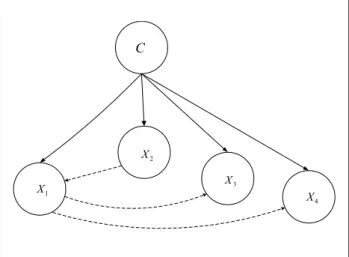
Figure 2 shows the structure of Svmguide1 data set, taken from LIBSVM, with four features (see Ta-ble 1) using the proposed algorithm. The solid lines are those edges required by the Naive Bayes classi-fier. The dashed lines are correlation edges between features found by our algorithm.
C 1 X 2 X 3 X 4 X
Figure 2: Proposed algorithm, Svmguide1
4 Discretization Algorithm Using
Sub-Optimal Agglomerative Clustering
(SOAC)
Discretization is a process which transform continu-ous numeric values into discrete ones. In this paper, we apply two different methods to discretize continu-ous features. The first one, whic