Android Malware Detection via Graphlet
Sampling
Tianchong Gao, Wei Peng, Devkishen Sisodia, Tanay Kumar Saha, Feng Li, Mohammad Al Hasan
Abstract—Android systems are widely used in mobile & wireless distributed systems. In the near future, Android is believed to dominate the mobile distributed environment. However, with the popularity of Android-based smartphones/tablets comes the rampancy of Android-based malware. In this paper, we propose a novel topological signature of Android apps based on the function call graphs (FCGs) extracted from their Android App PacKages (APKs). Specifically, by leveraging recent advances on graphlet mining, the proposed method fully captures the invocator-invocatee relationship at local neighborhoods in an FCG without exponentially inflating the state space. Using real benign app and malware samples, we demonstrate that our method, ACTS (App topologiCal signature through graphleT Sampling), can detect malware and identify malware families robustly and efficiently. More importantly, we demonstrate that, without augmenting the FCG with any semantic features such as bytecode-based vertex typing, local topological information captured by ACTS alone can achieve a high malware detection accuracy. Since ACTS only uses structural features, which are orthogonal to semantic features, it is expected that combining them would give a greater improvement in malware detection accuracy than combining non-orthogonal semantic features.Index Terms—Android; graphlet sampling; mobile applications; mobile malware; smartphone
F
1
INTRODUCTION
Some rising trends in mobile distributed systems, e.g., the wearable devices, the medical devices and the intelligent vehicle systems, are setup on Android platforms following the big success of it on smartphone market. Since Android applications written in Java are specifically designed to have as few implementation dependencies as possible, Android is believed to be adaptive to the new market and dominate the mobile distributed environment soon.
As the use of Android continues to grow, so does the threat of malware. Malicious behaviors observed in such malware include the theft of private information stored on the device, device fingerprinting, abusing premium service, and rooting the device as a backdoor for further attacks [39]. Detecting such malware is a critical task for the security research community.
It is observed that variants of malware form families through code sharing and their common lineage [39]. There-fore, instead of identifying individual malware and extract-ing a signature from it, we can identify the commonality within the same malware family and generate signatures that capture such commonality. Recently, various machine learning/data mining (i.e., pattern mining) techniques are • Tianchong Gao and Feng Li are with the School of Engineering and Technology, Indiana University - Purdue University Indianapolis, Indi-anapolis, IN 46202.
E-mail:{tgao, fengli}@iupui.edu
• Wei Peng is with the Intel Corporation, Folsom, CA 95630. E-mail: [email protected]
• Devkishen Sisodia is with the College of Arts and Sciences, University of Oregon, Eugene, OR 97403.
E-mail: [email protected]
• Tanay Kumar Saha and Mohammad Al Hasan are with the School of Sci-ence, Indiana University - Purdue University Indianapolis, Indianapolis, IN 46202.
E-mail:{tksaha, alhasan}@cs.iupui.edu
applied to detect Android malware [1, 2, 9, 19, 33, 36] or closely related tasks such as identifying repackaged apps [37, 38]. Beyond the common pattern mining frame-work, these works differ significantly in their selection and construction of features, their quantification/metrication of such features, their choice of pattern mining algorithms, and, in totality of these fine points of design, their appli-cability, robustness, and efficiency in detecting malware.
A number of different app representations have been studied for malware detection. For example, Yamaguchi et al. propose a compact representation of source code, the code property graph, that combines abstract syntax trees, control flow graphs, and program dependence graphs [33]. Other approaches do not require the source, but instead focusing on features at different abstract levels: from the low-level platform opcode level [36], through the inter-mediate function call [9] and Android framework API [1] level, to the high semantic level that includes features such as network addresses and Android specific artifacts such as permission and Intents [2]. Yet, other works formulate malware detection as different pattern mining tasks such as frequent subgraph mining [19].
Due to the availability of off-the-shelf obfuscation solu-tions (such as the free ProGuard [29] and the commercial DexGuard [28]) and the growing number of Android apps, it is critical for any proposed malware detection algorithm to be robust and efficient.
Robust. Malware detection should be insensitive to non-essential transformations. Non-non-essential transformations are program transformations that do not fundamentally turn an app into a different one. Examples of non-essential transformations include obfuscating long and descriptive function/method names by replacing them with short and meaningless ones [29], and re-branding through textual, pictorial, or animated resource replacement, or changing the ___________________________________________________________________
This is the author's manuscript of the article published in final edited form as:
Gao, T., Peng, W., Sisodia, D., Saha, T. K., Li, F., & Hasan, M. A. (2018). Android Malware Detection via Graphlet Sampling. IEEE Transactions on Mobile Computing, 1–1. https://doi.org/10.1109/TMC.2018.2880731
layout of the user interface [37].
Efficient.Malware detection should only take a reasonable amount of time to decide whether an app sample is malware or not. If the time is comparable with that of common com-mercial malware detection tools, we consider the malware detection method to be sufficiently efficient.
In practice, efficiency and robustness are often at odds. At one extreme, as two straightforward examples, crypto-graphical hashes or package names are highly efficient but fragile app signatures. They are efficient to obtain/compute but can easily be changed without essentially affecting the app [36]. At the other extreme, measuring similarities of some high-level graph-based representation of the app, such as code property graphs [33], are more robust, but, as ob-served by Gascon et al. [9], “is a non-trivial problem whose complexity hinders the use of these features for malware detection.”
Our first step towards robustness is to extract from the app under investigation its function call graph (FCG) [9], in which each vertex represents a Java method and each edge represents a method invocation. We concur with Gascon et al. [9] that FCG is at a proper abstraction level for detecting malware: In addition to the non-essential transfor-mations mentioned above, it is also immune to, for example, both lower-level opcode/instruction obfuscation or higher-level content encryption.
Based on the extracted FCG, we propose an efficient and robust Android app signature that faithfully captures the invocator-invocatee relationship between several functions, i.e., the topology of local neighborhoods on the FCG. Instead of using vertices and edges (or extension to 1-hop neighbor-hoods [9]) on the FCG “as is,” we leverage recent advances in graph mining to efficiently sample graphlets [23, 24] on the FCG. Graphlets are small (e.g., less than 6), con-nected, vertex-induced embedded subgraphs in an under-lying graph, which is the FCG in our case. In the spectrum of purely local (e.g., individual vertices/edges and simple metrics such as degrees) and fully global (e.g., between-ness centrality [3]) scope of the FCG, our graphlet-based signature takes a unique position: It faithfully captures local topological information at a fine-grained granularity without exponentially inflating the state space.
Given these characteristics, we call our graphlet-based signature a topological signature and, accordingly, name our method ACTS (App topologiCal signature through graphleT Sampling). In our experiments, ACTS achieves a cross-validated accuracy as high as 87.9% . In comparison, the same method with a purely local feature (i.e., degree frequency distribution (DFD) [7]) has an average cross-validated accuracy of 75%. Since ACTS only uses structural features, which are orthogonal to semantic features such as bytecode-based vertex typing, it is expected that combining them would give a greater improvement in malware de-tection accuracy than combining non-orthogonal semantic features.
Moreover, Android is going far beyond the smart-phones/tablets, e.g., the Android Wear, Android Pay and Android Auto. Some of the new applications are high level distributed systems that there are new rules and challenges for both the programming and the malware detection. In de-tail, the new malware detection method should be deployed
ω3 ,1 ω3 ,2 ω3 ,3 ω3 ,4 ω3 ,5 ω3 ,6 ω3 ,7 ω3 ,8 ω3 ,9 ω3 ,10 ω3 ,11 ω3 ,12 ω3 ,13
Fig. 1: The 13 unique 3-graphlet typesω3,i(i= 1,2, . . . ,13).
on various mobile distributed platforms and get analysis result swiftly. Since the topological features are related to the purpose of the software while the semantic features are highly connected to the programming languages and platforms, we believe that the method ACTS introduced in this paper is more adaptive to the new development but the dynamic analysis methods need additional work to follow the trend.
In summary, our contributions are:
• We propose a novel topological signature for Android apps that fully captures the invocator-invocatee rela-tionship in an app’s FCG, which is otherwise lost in a global topological metric such as betweenness central-ity [3], without exponentially inflating the state space as inn-hop neighborhoods withn≥3.
• By leveraging recent advances in graph mining, we make the generation of our proposed topological signa-ture practically efficient without sacrificing its robust-ness.
• With experiments on real malware/benign app sam-ples, we demonstrate that local topological information captured by our method alone can achieve a high mal-ware detection accuracy, which can be further improved by incorporating (orthogonal) semantic features. In the rest of the paper, after the preliminaries (Section 2), we present our method (Section 3) and experiment results on real malware/benign app samples (Section 4). We then reflect on our method (Section 5) and conclude with a brief review of related works (Section 6).
2
PRELIMINARIES
2.1 Function call graph
Function call graph (FCG) is a graph model for functions and their invocation relationship, in which vertices repre-sent functions and a directed edge from vertex v1 to v2
represents thatv1invokesv2. For an Android app, functions
are Java methods, and their invocation relationship can be statically extracted from Java bytecode by searching for the invocation-related opcodes, i.e., invoke-*.
2.2 Graphlets
Prˇzulj et al. first consider a complete set of local graph topologies with 3, 4, and 5 vertices and name them graphlets1 in their work on characterizing biological net-works [22]. Formally, given a graph G, graphlets of G
1. Graphlet is also used to refer wavelet decomposition of graphs [30], which is an unrelated concept to what we use in this work.
are small, connected, non-isomorphic, and vertex-induced subgraphs of G. Although earlier works [22, 23, 24] on graphlets focus on undirected graphs, we consider directed graphlets to preserve the inherent directionality of FCGs.
Figure 1 enumerates all the 13 unique types of (di-rected) graphlets ω3,i2 (i = 1,2, . . . ,13) with 3 vertices
(the 3-graphlets): They are pair-wise non-isomorphic. These graphlet types do not appear equally likely in an FCG. For instance, although there are many cases in which a function invokes two others (ω3,5) or two different functions invoke
the same one (ω3,6), 3 mutually recursive functions (ω3,13)
are rare. Later, we will discuss how we use this observation to improve the performance of our method (Section 3.3).
For vertices 4, 5, and 6, the number of graphlet types are 199,9,364, and1,530,843, respectively [26]. We focus on graphlets with less than 6 vertices in this work because larger graphlet types require extra computations but pro-vide little value in capturing the structure of FCG. Figure 2 illustrates our running example: A 4-graphlet g (the grey vertices and their induced edges) embedded in a 6-vertex graphG.
2.3 Graphlet frequency distribution (GFD)
Graphlet frequency distribution (GFD) of a graphGis the probability distribution of the frequencies of the different graphlet types in G. For instance, since the number of 3-graphlets in a (finite) FCG G is finite, we can, in princi-ple, enumerate all embedded graphlets inGand, for each such embedded graphlet g, identify g with one of the 13 graphlet types in Figure 1. At the end of the enumeration, suppose the count (i.e., the frequency) of graphlet type
ω3,i is f3,i (i ∈ {1,2, . . . ,13}), the frequency distribution
density d3,i at ω3,i is f3,i/P13i=1f3,i. We call the vector (d3,1, d3,2, . . . , d3,13)the 3-graphlet frequency distribution
(3-GFD) ofG. We can computen-GFD for anynwith the same procedure, and concatenate severaln-GFDs with differentn
into a single vector. We can call the concatenated vector a GFD ofGif there is no confusion on its constituents.
The above procedure only works in principle. In prac-tice, the fast growing number of apps, the size of real apps’ FCGs, and the combined computation complexity of graphlet enumeration and identify graphlet types make the enumeration-and-count procedure impractical to use. Nevertheless, GFD is a step forward towards our goal: It is a metrication from the (combinatorial) graphlet space into the (metric) Euclidean space, where we can apply pattern learning techniques to detect malware. In other words, GFD preserves the topological information of local neighborhoods in an FCG. Later, after giving a high-level overview of our method (Section 3.1), we will focus on how to estimate GFD efficiently (Section 3.2).
2.4 Minimum DFS code
Minimum depth-first search (DFS) code is proposed by Yan and Han to identify isomorphic graphs for frequent subgraph mining algorithm gSpan [34].
2. The unique types of n-graphlets are enumerated as
ωn,1, ωn,2, . . . , ωn,N(n), with N(n) being the number of unique
types forn-graphlets.
0 1
2 3
4 5
Fig. 2: Our running example: A 4-graphletg(the grey vertices and their induced edges) embedded in a 6-vertex graphG.
Essentially, for a graphG, by defining an encoding (i.e., the DFS code) for one3 DFS traversal of G, and a linear
order (i.e., the DFS lexicogrraphic order) for all possible DFS codes ofG, they prove that the minimum (under the DFS lexicographic order) DFS codeC(G):
C(G) = min{C(w)|all DFS traversalswofG}
is aunique encoding under isomorphism: Two graphsG1 and
G2are isomophicif and only if C(G1) =C(G2).
2.5 Metropolis-Hastings (M-H) algorithm
Markov chain Monte Carlo (MCMC) [10] is a class of algo-rithms for sampling from a probability distribution. Given an intended sampling distributionp(x)over a sample space
X, the idea behind general Markov chain Monte Carlo (MCMC) methods (in which the M-H algorithm is a specific method) is to construct a Markov chain over X whose stationary distribution equals to p(x): After the Markov chain mixes (i.e., reaches its stationary distribution and, hence, “forgets” where it begins), the subsequently visited states of the chain can be used as samples from the intended distributionP(x).
Metropolis-Hastings (M-H) algorithm [20] is a specific MCMC method that we use for estimating GFD (Sec-tion 3.2). In the M-H algorithm, the transi(Sec-tion between two consecutive states x and x0 in the chain consists of two stages: proposals and acceptance/rejection. Correspond-ingly, there is a proposal distributionq(x0|x)(the probability ofproposingx0as the next state given the current statex) and an acceptance distribution a(x0|x) = min(1, A(x0|x))(the probability ofacceptingx0as the next state given the current statex), in which:
A(x0|x) = p(x
0)q(x|x0)
p(x)q(x0|x). (1)
Intuitively, for each iteration of the sampling process, we first randomly pick x0 with a probability of q(x0|x), and then either acceptx0(by samplingx0) with a probability of
a(x0|x)or rejectx0 (by samplingxagain) with a probability of1−a(x0|x).
3
METHOD
In this section, after a brief overview of our method (Sec-tion 3.1), we zoom in on two technical points: Efficient GFD estimation (Section 3.2) and FCG-specific GFD dimension reduction heuristics (3.3) that distinguish our method.
3.1 Overview
Given an Android app’s APK (Android PacKage) binary package, we:
• extract an FCG from the APK,
• estimate the GFD of the FCG (Section 3.2), and
• project the estimated GFD to a lower dimensional space to reduce the GFD’s dimensions (Section 3.3).
The projected GFD, which is a vector, is a signature of the app. To stress that this signature preserves detailed topological information on an app’s FCG, we call it the
topological signature(TS) of the app.
Given a pool of both malware and benign app samples, we train a classifier on their TSs to detect malware: If the TS of an app is classified as a malware, the app is flagged as malware.
3.2 Efficient GFD estimation
Suppose we have a uniform sampler of the FCG, we can approximate the whole FCG’s GFD with our samples’ GFD. The more samples we take, the closer the approximation is. Given the large sample space and the (relatively small) number of bins (i.e., unique graphlet types) forn-graphlets withn < 6, we only need to sample a tiny fraction of the sample space to get a close approximation.
This apparently solve the GFD estimation problem. However, the real problem is that we need to uniformly
sample graphlets from the FCG without enumerating the sample space. Fortunately, two recent advances on graph mining, GRAFT [23] and GUISE [24], show that GFD can be estimated without enumerating all graphlets. Inspired by these works, we use MCMC to sample the directed FCG.
3.2.1 Sample space and intended distribution
Since our goal is to uniformly sample from all the embedded graphlets in the FCG:
• The sample space X consists of all the embedded graphlets in the FCG.
• The intended distribution p(x)overX is the uniform
distributions, i.e.,p(x) =p(x0)for anyx, x0∈X. Suppose we have just sampled graphlet g in the sam-pling process, the M-H algorithm (Section 2.5) says that, if we propose to sample graphlet g0 next with a
prob-ability of q(g0|g), an acceptance probability of a(g0|g) = min(1, A(g0|g))(in whichA(g0|g)is defined by Equation (1)) will eventually lead to a sampling process that have the desired sampling distributionp(x).
3.2.2 FCG-induced graphlet graph and graphlet neighbor-ing relationship
To define the proposal distributionq(x0|x), we consider the
FCG-induced graphlet graph GG of the FCG G. The FCG-induced graphlet graph GG is an undirected graph with vertices being all the embedded graphlets in the FCG, and edges defined by the graphlet neighboring relationship be-tween the vertices. The graphlet neighboring relationship is a symmetric relationship between two graphlet embeddings
g1andg2in the FCG:g1andg2are graphlet neighbors if and
only if they differ by share all but one vertex. In particular, self-neighboring is excluded by this definition because there is no vertex difference, which is required by the definition.
Since graphlets onGand vertices onGG have a one-to-one
map, we identify a graphletg onGwith the vertex onGG
that it maps to, and also denote that vertex withgif there is no confusion in the context.
For example, in Figure 2,g’s neighbors onGGare4all the 3-graphlets (e.g., {v2, v3, v4},{v3, v4, v5}, etc.), 4-graphlets
(e.g., {v1, v2, v3, v4}, {v0, v2, v4, v5}, etc.), and 5-graphlets
({v1, v2, v3, v4, v5}and{v0, v2, v3, v4, v5}) that share all but
one vertex with it. Conversely, 1){v1, v2, v3}is not a
neigh-bor ofgbecause it does not contain bothv4 andv5, which
are in g; 2) {v0, v1, v2, v3} is not a neighbor of g because
it does not contain g’s vertices v4 and v5 (and g does not
contain its vertices v0 and v1); 3) {v0, v1, . . . , v5} is not a
neighbor ofgbecausegdoes not contain its verticesv0and
v1.
The significance of the graphlet neighboring relationship onGGis that it can be efficiently generated bylocal informa-tionon the FCGGwithout enumerating the wholeG. Specifi-cally, given an embedded graphletgofG, the neighbors of
gonGGcan be generated by removing, changing, or adding
exactly one vertex ing. Hence, we can efficiently compute the degree dg ofg in GG by generating and counting g’s
neighbors.
3.2.3 Proposal and acceptance distributions
Letd(g)andN(g)be graphletg’s degree and neighbors in
GG, respectively. Suppose the last graphlet we have sampled
isg, our proposal strategyq(g0|g)is to uniformly sample one of its neighbors inGG, i.e.,
q(g0|g) =
( 1
dg ifg
0 ∈N(g),
0 otherwise. (2)
Sincedg can be efficiently computed without enumerating
the graph (see above), q(g0|g)can also be efficiently
com-puted since it only requires computingdg.
By Equations (1) and (2), the resulting acceptance strat-egya(g0|g)is: a(g0|g) = ( min(1,ddg g0) ifg 0∈N(g), 0 otherwise. (3)
By Equations (2) and (3), the probabilitys(g0|g)of sam-plingg0next given the current samplegis:
s(g0|g) = min(dg1,d1 g0) g 0∈N(g), 1−P h∈N(g)min( 1 dg, 1 dh) g 0=g, 0 otherwise. (4)
The intuition behind the sampling strategy in Equa-tion (4) can be understood in the following two cases.
Case 1.Ifgis a graphlet that has the highest degree among its neighbors in GG, i.e., dg ≥ dg0 for any g0 ∈ N(g), thenmin(1/dg,1/dg0) = 1/dg and, hence, by Equation (4), s(g|g) = 1−dg(d1
g) = 1−1 = 0, i.e., the next sample will notbegbut one of its neighbors.
Case 2.Ifgis a graphlet with a relatively low degree among its neighbors inGG,s(g0|g) in Equation (4) will be greater than 0. The greater the degree differences are, the greater 4. Given that graphlets are vertex-induced subgraphs, we use a vertex set to represent the (unique) embedded graphlet having those vertices here.
0.50
0.32
0.19
0.02
0.01
Fig. 3: The 5 3-graphlet types that have a greater-than-2% frequency density in the GFD of at least one app in our experiment, sorted by their average frequency density across all malware/benign app samples in our experiment.
0.23
0.20
0.10
0.05
0.03
~0
~0
~0
~0
~0
~0
0.01
~0
~0
~0
0.01
~0
0.02
0.29
0.07
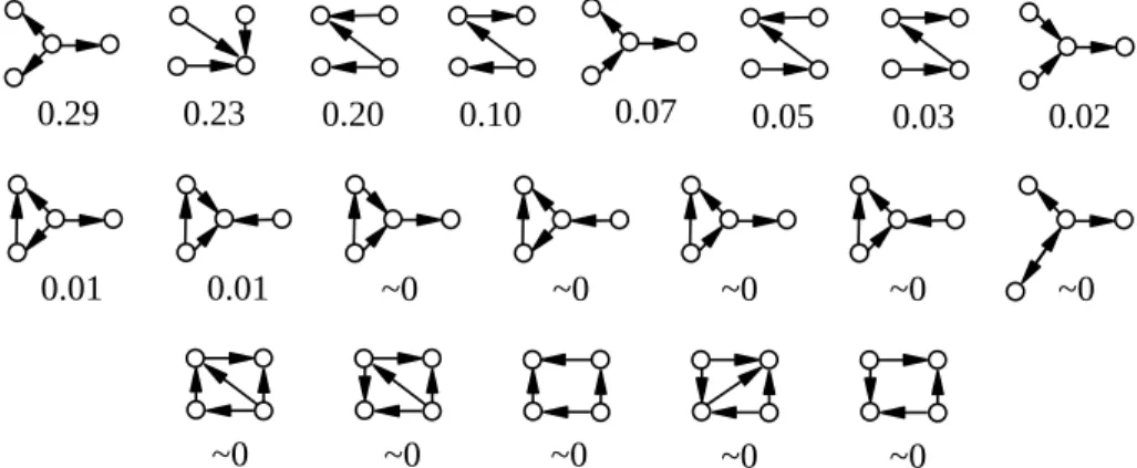
Fig. 4: The 20 4-graphlet types that have a greater-than-2% frequency density in the GFD of at least one app in our experiment, sorted by their average frequency density across all malware/benign app samples in our experiment.
Algorithm 1Estimate GFD for the FCGGfromtsamples. 1: IC: all thedistinctn-graphlet types forn∈ {3,4,5}
2: Ifc: frequency counter for graphlet typec∈ C
3: Idc: frequency density estimation for graphlet typec∈ C Input: G: the FCG;t: number of iterations
4:functionESTIMATE-GFD(G, T)
5: g←a random (initial) graphlet Ibootstrap the sampling process 6: NEXT-SAMPLE(G, g, T) Iobtain the vector(fc|c∈ C)
7: forc∈ Cdo Ifor each graphlet typec∈C
8: dc←fc/Pc∈Cfc Iestimate its graphlet density
9: end for
10: return(dc|c∈ C) I(dc|c∈ C)is a vector ordered byC
11:end function
Input: G: the FCG;g: current graphlet sample;k: remaining iterations 12:procedureNEXT-SAMPLE(G, g, k)
13: N(g)←g’s neighbors inGG ISection 3.2.2
14: choose ag0∈N(g)with an equal probability of1/d
g IEquation (2)
15: a←a number uniformly sampled from[0,1] 16: ifa≤min(1, dg/dg0)then Iacceptingg0
17: g←g0
18: else Irejectingg0
19: end if
20: c← C(g) Iidentify (the new)g’s type 21: fc←fc+ 1 Iincreaseg’s count
22: ifk >0then Iif there are remaining iterations
23: NEXT-SAMPLE(G, g, k−1) Iwe continue the sampling process 24: end if
25:end procedure
s(g0|g) will be. In an extreme case in whichg has a single neighborg0with a degree of 100 (i.e.,dg= 1anddg0 = 100), s(g0|g) = 0.01ands(g|g) = 0.99: If the current sample isg,
99 out of 100 times, the next sample will still beg.
In other words, the sampling process (i.e., the consecu-tive states of the Markov chain) is more eager tomove away fromthe more popular graphlets (i.e., the ones with higher degrees in GG) and to stay at the less popular ones: The former has a better chance than the latter of being revisited later. This results in a fair (i.e., uniform) sampling of all the embedded graphlets in the FCGG.
3.2.4 Minimum DFS code for directed, unlabeled graphs
An important step of our method is to differentiate the graphlets in sampling. A naive approach is to apply di-rected graph isomorphic recognition algorithms. Although
our sapling space is limited to graphlets with no more than 5 nodes, naively recognizing isomorphism graphs is still a complex work. Hence, we introduce the minimum DFS code, which is proposed by Yan and Han (Section 2.4), to identify subgraph isomorphism on an undirected and labeled graph.
To handle the FCG’s inherent directness, we extend the definition of DFS lexicographic order to include an encoding of the edge directionality. Specifically, suppose the ordered edge sequence in the DFS codeC(GT)for the graph
traver-salGT ise1, e2, . . . , e|E|(with the encoding of edgeeibeing (vi,1, vi,2)), we attach an|E|-tuple(d1, d2, . . . , d|E|) to the
end ofC(GT).diencodes the directionality ofei:
di =
0 the direction is fromvi,1tovi,2,
1 the direction is fromvi,2tovi,1,
2 eiis a bi-directional edge..
This extension captures the directionality of edges and fits naturally into the minimum DFS code generation algo-rithm [34]. Without inflating our symbols, we use C(G)
henceforth to represent our extended minimum DFS code. For example, in Figure 2, the minimum DFS code for the 4-graphlet embeddinggis:
C(g) = (0,1)(1,2)(2,0)(2,3)|(0,0,0,1),
in which verticesv2,v3,v4, andv5are encoded as 0, 1, 2, and
3, respectively. The 4-tuple at the end encodes the directions of the edges(v2, v3),(v3, v4),(v4, v2), and(v4, v5):v2→v3,
v3 → v4,v4 → v2, andv4 ← v5. Any 4-graphletg0 that is
isomorphic togwill have the same minimum DFS code, i.e.,
C(g0) =C(g).
In the naive subgraph isomorphic recognition algorithm, the target graph should be compared with each candidate graphlet. For instance, a 5-node graph has 9,364 possi-ble matching. Advanced subgraph isomorphic recognition algorithms, e.g., Frequent Subgraph Discovery (FSD) and minimum DFS code, pruned the search with labeling the
subgraphs [14, 34]. Moreover, the minimum DFS code gen-eration algorithm applies the DFS search to efficient mine frequent connected subgraphs. This algorithm has 6-150 speed-up in comparison with FSD algorithm [34].
3.2.5 GFD estimation algorithm
Finally, we estimate the GFD for the FCGGfromtsamples by evaluating ESTIMATE-GFD(G, t)in Algorithm 1. In our experiment, we evaluate multiple t and choose 100,000
for having both low variance in the sampling result and acceptable efficiency. Note that, given the average size of an FCG G (thousands of vertices) and, hence, the sample space GG (for a 1,000-vertex G,GG has a worst-case size
of O(1,0003)), 100,000 iterations are quite small. Indeed, for the largest app in our dataset (the Facebook app, with
47,539 vertices and 77,900 edges), ESTIMATE-GFD(G, T)
forT = 100,000only takes only about 34 seconds on our desktop workstation with high convergence across multiple runs.
3.3 FCG-specific GFD dimension reduction heuristics
The curse of dimensionality [12] plagues many machine learning tasks. Theoretically, by confining the n-graphlets we sampled to n ∈ {3,4,5}, the GFD vectors we obtain from Algorithm 1 are of9,576(13+199+9,364; Section 2.2) dimensions. Reducing the dimensions of these vectors is desirable.
Fortunately, as briefly discussed in Section 2.2, not all graphlet types are equally likely to appear in a real FCG. Figures 3 and 4 show all 3-graphlet and 4-graphlet types (5-graphlet types are omitted for space constraints) that have more a greater-than-2% frequency density in the GFD of
at least one of the (more than 1,400) apps (including both malware and benign apps) in our experiment: There are 5 3-graphlet types, 20 4-3-graphlet types, and 71 5-3-graphlet types, respectively.
Note that, as we discuss in Section 2.2 and is verified here, graphlet types ω3,5 (outgoing invocations) and ω3,6
(incoming invocations) rank among the most frequent 3-graphlet types, while the mutually recursive type (ω3,13) is
not. Moreover, except for a few cases of mutual recursion, loops among a few functions of are rare. This suggests that: 1) either inter-function loops have a long chain of invocations, 2) or most functions have a clear invocator-invocatee relationship that is not reciprocal.
These observations suggest that we can significantly cut down the dimensions of GFDs by projecting the GFD vectors onto themost frequent dimensions. Indeed, this is what we do in our method after obtaining the full-spectrum (i.e.,
9,576-dimensional) GFD estimation.
4
EXPERIMENT
RESULTS
4.1 Datasets
In our experiment, we use the benign app samples from PlayDrone [32] and use the malware samples from the Android Malware Genome Project (AMGP) [39].
For the benign app portion of our datasets, we download the dataset of PlayDrone. There are total 49000 benign sam-ples in 9 different archives. To test the scalability and robust
RBF Linear Polynomial Sigmoid 60 70 80 90 100 Kernel Type Accuracy (%)
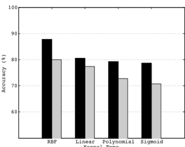
Fig. 5: Malware detection accuracy of SVM-GFD (SVMs with GFD-based signature; dark) and SVM-DFD (SVMs with DFD-GFD-based sig-nature; grey) using C-SVC (C-support vector classification) SVMs (support vector machines) with different kernels: RBF (radial basis function), linear, polynomial, and sigmoid.
TABLE 1: Malware detection false positives (FPs) and false negatives (FNs): SVM-GFD vs. SVM-DFD with different kernels.
RBF linear FP FN FP FN GFD 11.53% 12.78% 19.30% 19.55% DFD 13.03% 27.07% 17.54% 27.82% polynomial sigmoid FP FN FP FN GFD 20.80% 20.55% 22.01% 20.55% DFD 21.30% 33.08% 26.57% 32.08%
of our algorithm, we randomly and repeatedly choose sets from the PlayDrone and each set has thousands of benign samples. We also check the package name, the version code and theM D5message of each sample to prevent the duplicate in it. For the malware portion of our datasets, the AMGP lists1,249malware samples of 49 families.
4.2 Procedure
We first use Androguard [15], an Android app reverse engineering toolkit, to extract FCGs from the APK sam-ples. Specifically, we use theandrogexf.pyscript to extract a GEXF5-format file that encodes the Java methods and their
invocation relations in the APK.
We implement our GFD estimation algorithm (Algo-rithm 1) to generate a GFD vector for all n-graphlet types for n ∈ {3,4,5}. The majority of dimensions have a fre-quency of 0; hence, we use the FCG-specific GFD dimension reduction heuristics (Section 3.3) to reduce these 9,576 -dimensional vectors to 96-dimensional ones (details are shown in Section 4.3.3). These 96-dimensional vectors are the topological signatures of their corresponding apps.
We then use the LIBSVM [4] support vector machine (SVM) library for classification; the details are mentioned below along with corresponding results.
4.3 Results
To understand how the local-topology-preservation prop-erty of GFD helps in enhancing malware detection perfor-mance, we compare our method with another method in 5. GEXF (Graph Exchange XML Format); http://gexf.net/format/.
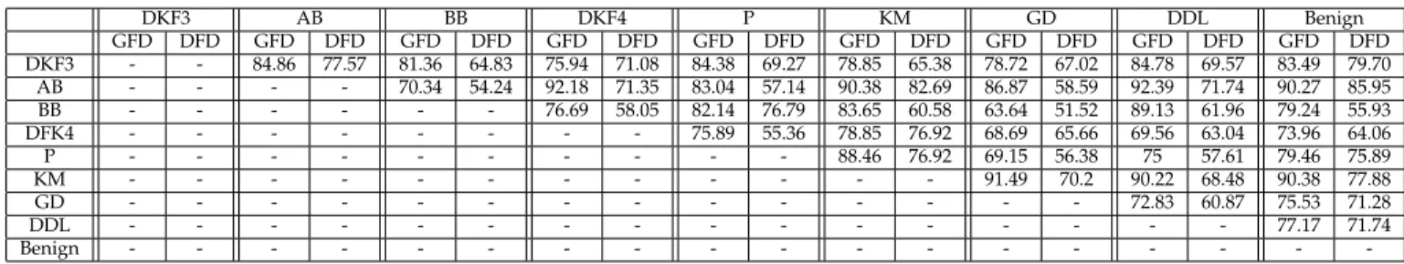
TABLE 2: Pair-wise malware family label accuracy (in percentage) of SVM-GFD (GFD) vs. SVM-DFD (DFD) with the RBF kernel of the 8 malware families that have over 40 samples in the AMGP dataset: DroidKungFu3 (DKF3; 303 samples) AnserverBot (AB; 185 samples), BaseBridge (BB; 118 samples), DroidKungFu4 (DKF4; 96 samples), Pjapps (P; 56 samples), KMin (KM; 52 samples), GoldDream (GD; 47 samples), and DroidDreamLight (DDL; 46 samples). Since this matrix is symmetric, we only show the upper half of it.
DKF3 AB BB DKF4 P KM GD DDL Benign GFD DFD GFD DFD GFD DFD GFD DFD GFD DFD GFD DFD GFD DFD GFD DFD GFD DFD DKF3 - - 84.86 77.57 81.36 64.83 75.94 71.08 84.38 69.27 78.85 65.38 78.72 67.02 84.78 69.57 83.49 79.70 AB - - - - 70.34 54.24 92.18 71.35 83.04 57.14 90.38 82.69 86.87 58.59 92.39 71.74 90.27 85.95 BB - - - 76.69 58.05 82.14 76.79 83.65 60.58 63.64 51.52 89.13 61.96 79.24 55.93 DFK4 - - - 75.89 55.36 78.85 76.92 68.69 65.66 69.56 63.04 73.96 64.06 P - - - 88.46 76.92 69.15 56.38 75 57.61 79.46 75.89 KM - - - 91.49 70.2 90.22 68.48 90.38 77.88 GD - - - 72.83 60.87 75.53 71.28 DDL - - - 77.17 71.74 Benign - - -
-which both the (preceding) FCG extraction phase and (sub-sequent) learning phase are the same. The only difference is the feature we extract from FCG. Specifically, we use the degree frequency distribution (DFD) for comparison. In DFD, vertices with the same degree frequencies are binned together and counted. DFD is the probability distributions of element counts over these bins. In other words, the only difference between the two methods is whether local topol-ogy information of FCG is used in the subsequent learning phase: Our GFD-based method uses this information, while the DFD-based method does not.
For reasons that will be explained shortly, in this ex-periment, we randomly and repeatedly pick 1200 samples from the benign dataset to compare with the 1200 malware samples. In each comparison, we use the 10-fold cross verifi-cation, which means that each time 120 benign samples and 120 malware samples are randomly chosen as test set, other samples will be feed as training set and the result shows the overall average accuracy. Then we compare malware detection performance of SVMs with GFD-based signatures GFD) and SVMs with DFD-based signatures (SVM-DFD) using all 4 built-in SVM kernel functions in LIBSVM: RBF (radial basis function:eγ|u−v|2
), linear (u0·v), polyno-mial ((γu0 ·v)3), and sigmoid (tanh(γu0 ·v)), in which u
and v are feature vectors, γ = 1/N, and N is the feature vector dimension. Figure 5 shows the accuracy (the samples that are correctly labeled by the SVMs) comparison and Table 1 shows the detailed false positives/negatives (the samples that are incorrectly labeled by the SVMs). We do observe similar results on the repeated experiments but we just choose to report one due to the space constraint.
4.3.1 Malware detection performance
The reason we use a 1:1 ratio between malware and benign app dataset is that a skewed dataset may give misleading performance results. Later in this part we will also present the influence of sample bias. In both Figure 5 and Table 1, the performance of SVM-GFD and SVM-DFD appear to be consistent across learning kernels. The high accuracy of the two algorithms implies that both of them could successfully capture topological features, and the features are helpful to Android malware detection.
Comparing these two algorithms, SVM-GFD always give better results (by average 6% margin over the SVM-DFD algorithm, to over 80% accuracy). A recent study [2] on commercial anti-virus scanners’ (AntiVir, AVG, BitDe-fender, ClamAV, ESET, F-Secure, Kaspersky, McAfee, Panda,
Sophos) performance on the AMGP dataset shows that, except for two outliers (23.68% and 1.12%), the commercial AV scanners have accuracy ranging from 84.23% to 98.90%. SVM-GFD attains a comparable accuracy of 87.85% on the full AMGP dataset using only the structural features with-out any semantic augmentation.
Figure 5 suggests that RBF kernel could give a better result than other three kernels both for GFD and SVM-DFD. SVM-GFD could perform a 78% or higher results on different kernels, while SVM-DFD shows 70% accuracy when choosing polynomial or sigmoid kernel. So the SVM-GFD seems more robust than SVM-DFD. Table 1 shows that they have different performance among false positives (FP) and false negatives (FN). Because the dataset is 1:1 ratio, FP and FN achieving a nearly 1:1 ratio means the SVM could successfully divide the hyperplane. From Table 1 we can see that these two SVM methods tend to give high accuracy under the specified circumstances. And SVM-GFD often have a same FP or FN percentage as SVM-DFD while the other is much better.
4.3.2 Malware family labeling accuracy
To further understand the significance of capturing local topology in FCG for malware detection, we compare our SVM-GFD together with the SVM-DFD in their malware family labeling accuracyon the 8 malware families that have over 40 samples in the AMGP dataset. Specifically, we take the family labels on the malware samples in the AMGP dataset as the ground truth, and compare the two methods’ accuracy in assigning the correct family labels for the test data sets. Here we use 3-fold cross verification instead of the 10-fold one because some families, e.g., GoldDream with 47 samples, do not have enough samples to be divided into 10 folds. And we use the same number of samples, which is the size of the smaller family, from two families in comparison. We also compare each family with a dynamic benign dataset, which is viewed as another kind of ‘mal-ware’ family. Therefore, the last column result shows the accuracy of malware detection in one certain family.
Table 2 shows the pair-wise (one vs. one) malware family labeling accuracy of SVM-GFD vs. SVM-DFD with the RBF kernel, since both methods get the best results with the RBF kernel (Section 4.3.1). GFD outperforms SVM-DFD in all pairs of malware families by a margin from 1.93% (DKF4/DroidKungFu4 vs. KM/KMin) to 27.17% (BB/BaseBridge vs. DDL/DroidDreamLight). The malware and benign software classification result in each family also
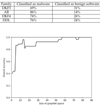
TABLE 3: Classification result of unknown family Family Classified as malware Classified as benign software
DKF3 69% 31%
AB 86% 14%
DKF4 74% 26%
DDL 76% 24%
Fig. 6: Accuracy against different sampling size
shows SVM-GFD could achieve 3.57% (P/Pjapps vs. Benign) to 23.31% (BB/BaseBridge vs. Benign) higher performance. Note again, the additional local topological information on FCG captured by GFD, alone, takes the credit for this improvement in accuracy.
When an unknown sample, which does not belong to known families, appears, we do experiment to test the detection accuracy to examine if we need to re-train the model. In this experiment, we manually eliminate some malware families from the training dataset and use them as the test dataset. The detection accuracy is shown in Table 3. The results show that even if the sample belongs to an unknown family, our SVM-GFD model is still available to detect the malware with probability 69% and above.
Also, another experiment shows that if we re-train the SVM-GFD model with samples in that family, the model has an accuracy of 100% to detect the malware. By comparison, the detection accuracy is about 75% in classifying malware within one family with benign software, which is shown in the last two columns of Table 2. The improving of detection accuracy implies that malware from other families also contribute to the classification. This is also the reason of the robustness of our method when the family is unknown to the model.
4.3.3 Performance against sampling space size
In Section 3.3, we reduce the graphlet space dimensions from 9,576 to 96, because of the reasons: the reduced features have low frequency density in GFD space, and the space after reduction can give accurate malware detection. For the first reason, we analyze the graphlet space of more than 1,400 Android apps. The 96 graphlets are chosen because they have at least 2% frequency density in at least one app. For the second reason, we analyze the detection accuracy with different sampling space sizes based on a toy dataset with 200 apps.
(a) The distribution of number of nodes
(b) The distribution of number of edges Fig. 7: FCG sizes of benign apps and malicious apps
Figure 6 shows the analysis result. We can find that when the graphlet space is small, i.e., with less than 5 dimensions, the detection accuracy is not better than a naive strategy which classifies all apps into benign (or malicious). However, the graphlet spaces with more than60dimensions have stable and effective performance in malware detection. This experiment encourages us to apply GFD dimension reduction heuristics.
4.3.4 Performance against graph size bias
There is a huge difference of the sizes between the benign apps and malicious apps. While common benign APK files have the size of 1MB to 10 MB, the malicious APK files are usually hundreds of KB. Most of the malicious applications only care about their malicious functions, whose size are small compared with the source code of the benign applica-tions. Although our classification is based on FCGs, the size difference in Android APKs will result in the size difference in FCGs. There are several metrics to measure the size of a graph, e.g., the number of nodes and the number of edges. Figure 7 shows the distribution of the FCG sizes. The result demonstrates that the malicious apps always have smaller FCGs than the benign apps. The average number of nodes is 1348 in the malicious apps but it is 10046 in the benign apps. The numbers of edges are 1919 and 14180 of the malicious
(a) Accuracies of graphs with different node number
(b) Accuracies of graphs with different edge number
(c) Accuracies of graphs with different max degree Fig. 8: Accuracies of graphs with different sizes
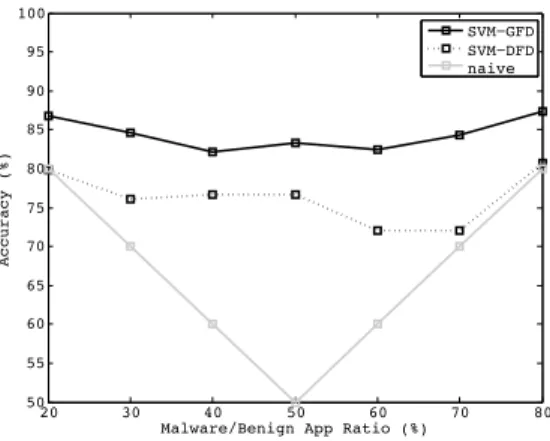
20 30 40 50 60 70 80 50 55 60 65 70 75 80 85 90 95 100
Malware/Benign App Ratio (%)
Accuracy (%)
SVM−GFD SVM−DFD naive
Fig. 9: Accuracy response to different malware/benign-app ratios: SVM-GFD (full line) vs SVM-DFD (dotted line) vs the naive strategy. Percentage on thexaxis is the ratio of malware over benign apps in the dataset;yaxis is the malware detection accuracy.
apps and benign apps, respectively. Considering the average case, the benign apps have FCGs about 7 times larger as the FCGs of the malicious apps.
Thus, one may argue that the difference in FCG sizes, instead of the structure difference between the malicious apps and benign apps, leads to the high performance of the detection. Figure 8 shows the detection accuracies when the malicious apps and benign apps have different sizes of FCGs. We take three metrics to measure the size of a graph: the node number, the edge number, and the max degree in the graph. The scale of grey shows the accuracy: white is 100% accurate and black is 0% accurate. In the result, most of the results achieve 80% accurate or higher. In Figures 8(a) and 8(b), there is no significant trend that the accuracy of different sizes of graph is higher than the accuracy of similar sizes of graphs. For example, the accuracy of classifying 100 nodes malicious FCGs with 900 nodes benign FCGs is not higher than the accuracy of classifying 900 nodes malicious FCGs with 900 nodes benign FCGs.
However, in Figure 8(c), we can find that the accuracies on the diagonal are always smaller than the accuracies on the two conners. It means that the differences in the max degree of the graph significantly impact our detection results. Considering that the detection is based on the GFD, we find that the graphlet frequency distribution is correlated with the max degree in the graph. Combining the results in Figure 8(a) and 8(b), we can conclude that our detection accuracy, i.e., the FCG’s GFD, is not directly linked with the graph size, but it is related with the density of the graph.
4.3.5 Performance against sample bias
In Section 4.3.1, we mention the peril of sample bias: If the ratio between positive and negative samples (i.e., benign app and malware samples) is skewed, even a naive strategy can give a misleadingly high accuracy without actually identifying malware from benign apps. In real-world mal-ware detection, positive/negative samples rarely comes in evenly: It is highly likely we have to work with a skewed dataset.
Therefore, we study how SVM-GFD responds to sample bias. In order to avoid the influence of the dataset’s size, we
TABLE 4: Recall with keeping high precision RBF linear fixed precision 80% 90% 100% 80% 90% 100% GFD recall 62% 42% 38% 28% 0% 0% DFD recall 0% 0% 0% 0% 0% 0% polynomial sigmoid fixed precision 80% 90% 100% 80% 90% 100% GFD recall 80% 6% 6% 48% 24% 6% DFD recall 8% 6% 6% 4% 4% 4%
first fix the total number of benign and malicious softwares to 1000. Then we perturb the ratio between malware and benign app samples, and study the accuracy response of SVM-GFD/SVM-DFD with the linear kernel. Figure 9 shows the results and indicates that SVM-GFD gets higher accu-racy among all kinds of malware and benign software com-bination. SVM-GFD has a variance of 4.1 while SVM-DFD has a variance of 11.4. We conclude that SVM-GFD is more robust than SVM-DFD against sample bias, especially when malware or benign software accounts a small proportion. When the ration between malware and benign software is 2:8, as mentioned above it is a common real-world situation, SVM-GFD outperforms 7% accuracy but SVM-DFD is just the same as the naive strategy.
4.3.6 Recall with keeping high precision
In practical cases, not only is the sample dataset skewed (large number of benign samples and small number of malicious samples), but also the malware detection method is expected to have high precision and recall. In this section, we fix precision to a high value and examine recall of SVM-GFD/SVM-DFD results. These results show the ability of the proposed methods to reduce false negatives with little precision loss. Moreover, in order to eliminate the performance gain of skewed dataset and simulate real cases, we choose a biased training dataset with 90% of benign samples, but a unbiased test dataset with 50% malware.
In this experiment, we fix the precision to 80%, 90%, and 100% and get the recall of the two methods. Each number in Table 4 shows an average recall of ten different experiments. Each experiment uses 10% disjoint dataset as the test data, which is similar to 10-fold cross verification. SVM-GFD achieves higher recall value. When the detection is required to have 100% precision, SVM-GFD can get 38% recall with the RBF kernel. By comparison, SVM-DFD only gets 6% recall when the detection requires 100% precision. It means that SVM-GFD achieves relatively high true positives without false positives compared to SVM-DFD method.
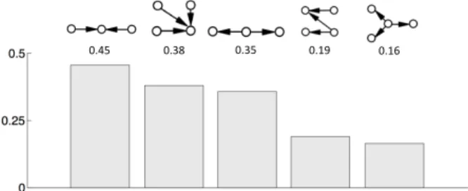
4.3.7 Most frequent graphlets
To understand why malware detection accuracy improves only by replacing DFD with GFD, we study the most fre-quent graphlets that appear in benign apps and in malware. Figures 10 and 11 show the top 5 most frequent graphlet types for all benign app and malware samples in our datasets, respectively. “Most frequent” in this case means that these graphlet types have the highest average GFD densities in that category (benign app or malware).
It is interesting to note that, in addition to different average density values, the types of the most frequent graphlets are different. For example, while ω3,5 (outgoing
0.45 0.38 0.35 0.19 0.16
Fig. 10: The top 5 most frequent graphlet types for benign apps, i.e., the ones that have the highest average graphlet frequency densities across all benign apps.
0.52 0.31 0.26 0.19 0.19
Fig. 11: The top 5 most frequent graphlet types for malware, i.e., the ones that have the highest average graphlet frequency densities across all malware.
invocations; Figure 1) ranks the first and w3,6 (incoming
invocations) ranks the third for malware, ω3,5 ranks the
third andω3,6ranks the first for benign apps. In both cases,
these two graphlet types have a graphlet frequency density gap of 0.1 or more between them. And it also happens when a function invokes/is invoked by 3 or more other functions. This suggests that incoming invocations to a same function is more frequent than outgoing invocations from a single function in benign apps, while the reverse is true for malware. The mechanism behind this calls for further research.
4.3.8 Robustness with SVM parameters
When the two methods are used to detect malware in new datasets, the SVM may not be well-trained. It is important for the SVM to have the robustness. In this part, e compare the GFD and DFD methods with various SVM parameters. Here we use the RBF kernel, which has the highest per-formance in classification, as the example. The RBF kernel has two parameters, the cost C and the Gamma γ. The cost takes a trade-off between the misclassification rate and the simplicity of the detection surface [6]. Lower the cost, simpler the decision surface, but higher the misclassification rate with the training dataset. Theγis the one ineγ|u−v|2
.γ
changes the influence of a single example, which is chosen to be the support vector. Higher theγ, higher the influence of the example.
Figure 12 shows the accuracy results of the two methods. Similarly, the scale of grey shows the accuracy: white is 100% accurate and black is 0% accurate. The accuracies of the GFD results are all above 70%, while some DFD results are only 53% accurate.
(a) Accuracies of the GFD method
(b) Accuracies of the DFD method Fig. 12: Accuracies with different SVM parameters
We also evaluate theF1-score of the two methods, which
is the average of the recall and the precision.
precision= T P T P +F P recall= T P T P +F N F1= 2· precision·recall precision+recall = 2T P 2T P +F P+F N (5)
Figure 13 show theF1-scores of the two methods. TheF1
-scores of the GFD results are all above 0.65, while the DFD results have 0.16 F1-scores when the cost and gamma are
not suitable. We find that when cost and gamma are small, the false positive rate of the DFD results is high. The DFD method lacks enough robustness to classify the malicious applications. When the SVM is not well-trained for the test dataset, the DFD method has high possibility to raise alarms to benign applications. On the contrary, our GFD method has enough robustness to new datasets.
(a)F1-scores of the GFD method
(b)F1-scores of the DFD method
Fig. 13:F1-scores with different SVM parameters
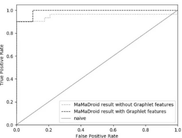
4.3.9 Combination with semantic analysis tool
Since ACTS uses structural features, which are orthogo-nal to semantic features, combining ACTS with semantic analysis tools is expected to give a great improvement in malware detection accuracy. In this experiment, we combine our method with MaMaDroid, a state-of-the-art malware detection method using semantic features [18].
Specifically, MaMaDroid abstracts each Android func-tion into package or family. For instance, the funcfunc-tion
com.beyondar.world:getInstance has the family com and the packagecom.beyondar. Then MaMaDroid embeds a Markov Chain to model the sequence of these functions. Because MaMaDroid mainly focus on the semantic features, this algorithm is suitable to connect with our structural analysis tool. In this experiment, we inject the GFD frequency distri-bution as additional features to show if the combination tool can get better detection performance. The result is shown in Figure 14. When directly applying MaMaDroid, the area under the Receiver Operating Characteristic (ROC) curve is 0.95. If the two analysis tools are combined together, the area under ROC curve is 0.99. It proves that our method is an enhancement to existing semantic analysis tools.
Fig. 14: ROC curve of detection result combining with MaMaDroid
Fig. 15: Feature extraction time of different methods
4.3.10 GFD estimation efficiency
Figure 15 shows the feature extraction time of different methods among different sizes of FCGs, in our experiment on a desktop workstation (8-core Intel Core i7-3820 CPU at 3.60GHz with 12GB RAM) with 100,000 sampling it-erations (at which point, the GFD estimation has already converged). Because GFD-SVM method and MaMaDroid apply the MCMC algorithm to approximate the true dis-tribution of GFD or FCG connection, these two methods have consistency in runtime with different sizes of FCGs. On the contrary, DFD-SVM method needs to capture the degree distribution, which is a global feature and not suitable to MCMC sampling. While MaMaDroid focuses on the func-tion call relafunc-tionships themselves, our GFD-SVM method extracts the graphlets which are more complex [18]. Hence, the extraction time of our GFD-SVM method is longer but it is still acceptable.
While the GFD estimation just takes seconds of work to analyze each single app, the total calculation time mainly depends on the size of the dataset. Because all apps and their FCGs are independent with each other, the topolog-ical features extraction work is absolutely convenient for distributed computing system. And the overall system is
expected to be more efficient if it is setup on a cloud computing system with more powerful servers. Analyzing single extraction work, we note that GFD estimation is dominated by the generation of 1-hop neighborhood onGG
and the minimum DFS code computations (for graphlet-type identification), which are independent to the size of the graph unless the graph is dense.
By contrast, the DFD calculation needs to traverse every edge and employ a sorting algorithm to the vertices. So it takes more time to do the DFD calculation especially on the complex networks. For instance, DFD calculation takes about 41 seconds for the Facebook application, 7 seconds longer than the GFD estimation. Therefore, GFD estimation, and hence ACTS, is practically efficient and accurate (Sec-tion 1).
The efficiency and accuracy also drive us to move the de-tection platform to Android itself. It seems possible that each smartphone could analyze its own applications because the total size of analysis tool is relative small (ACTS is 65MB and a vector of 1000 software samples is about 2MB). Deploying such distributed detection system will allow us to aggregate and analyze the software swiftly.
5
FURTHER
DISCUSSION
5.1 Static features extraction
The essence of ACTS is the FCG-local-topology-preserving feature based on GFD, on which pattern mining techniques can be applied. Its effectiveness for malware detection can be better understood by relating it to the following ideas on extracting graph features.
Subgraph isomorphism. Subgraph isomorphism can be applied to determine whether two FCGs share common sub-structures. Besides its NP-completeness [5], it is not robust against even minor perturbation (e.g., breaking a large func-tion into a few smaller ones during code refactoring) in the FCG due to the binary nature of its result, e.g., yes or no to “whether two FCGs share an isomorphic subgraphs with 5 vertices.”
Betweenness centrality. Betweenness centrality [3]) mea-sures relative topologically importance of the vertices in the FCG. Although betweenness centrality captures the large picture of the graph topology, it also loses information on the FCG at the level of a few neighboring vertices. This nuance is important for detecting malware.
Degree frequency distribution. Degree frequency distri-bution (DFD) [7] is the distridistri-bution of the frequencies of vertex degrees. DFD can be efficiently computed by a single walk over the vertices in the graph. However, by focusing solely on vertices, DFD loses the topological information in an FCG, which includes, for example, directionality and the invocation relationship between several functions. Our experiments (Section 4) demonstrate the importance of such topological information for detecting malware.
n-hop neighborhood. An n-hop neighborhood is a sub-graph with a diameter ofn, i.e., the maximal shortest (edge) distance between any pair of vertices in the subgraph isn. Its granularity in relation to the parameternis too coarse for our task. For instance, a 3-hop neighborhood can be much larger than a 2-hop one.
5.2 Case study of dynamic analysis
In order to verify the effectiveness of the graphlet-based analysis and to better understand why the topological fea-tures used in ACTS could result in good performance of benign/malicious software classification, we also conducted a few case studies using dynamic analysis that based on semantic features [27].
The motivation of combining the static and dynamic analysis in Android malware detection is from the desire of taking the advantages of the two methods. Particularly, dynamic analysis allows us to run the applications live. The dynamic analysis tools inspect the behavior of the applications. Dynamic analysis tools, e.g., Andrubis and SandDroid, are capable to provide the malicious function calls [17, 31]. Static analysis allows us to do reverse engi-neering. Static analysis tools, e.g., Androguard, provide the information of app permissions, Java methods, and their invocation relationships.
In the case study, we obtain the critical API calls with the help of online analysis tools. These critical calls are represented as edges in the FCG. And if a function invokes one of more times of the critical API calls, we label the mapping vertex as a critical vertex. Instead of taking the full FCG graph into account, now we can just focus on the graphlets that contain the critical vertices.
Our experiment were taken on four APK files randomly chosen from four different malware families, TapSnake [21], SndApps [13], NickySpy [11] and LoveTrap [16]. The result shows that for each particular malware, its top-2 graphlets with critical vertices are always the same as the top-2 graphlets in GFD generated by ACTS. And obviously, they are different from the top-2 graphlets generated from the be-nign softwares. It implies that the most frequent graphlets of malware generated by ACTS in Section 4.3.7 always contain the critical API calls. These graphlets are the attacking core of a malware.
We also in-depth analyzed one application
com.typ3studios. airhornin the malware family SndApps [13]. There are just four critical graphlets that were obtained through dynamic analysis tools. After embedding the 3-node graphlets in 4&5-node graphlets, we find that there are only 2 kinds of 3-node graphlets that contain the critical API calls, ω3,5 and ω3,1 in Figure 1, while the
possible 3-node graphlets has 13 types. Also,ω3,5(outgoing
invocations) is included but w3,6 (incoming invocations)
is not. It supports the result in Figure 11 of Section 4.3.7 that outgoing invocations to a same function is more frequent than incoming invocations from a single function in malware. In the future, we plan to add more cases in the experiment to find the hidden mechanisms of malware by combining both the static and the dynamic analysis.
6
RELATED
WORKS
The present work follows a line of recent works [1, 2, 9, 19, 33, 36] that apply advances in machine learning and data mining for Android malware detection. Some of them were based on semantic information, which in-cludes the signatures, API calls, opcode, and Java methods. DroidAPIMiner focused on API level information within the bytecode since APIs convey substantial semantics about
the apps behavior [1]. More specifically, DroidAPIMiner extracted the information about critical API calls, their pack-age level information, as well as their parameters and use these features as the input of classification. Droid Analytics designs a signature based analytic system [36]. This system can automatically generate the signatures based on the in-put Android application’s semantic meaning at the opcode level. Unlike previous signature-based approaches, which are vulnerable with bytecode-level transformation attacks, Droid Analytics can defense against repackaging, code ob-fuscation, and dynamic payloads [25]. Drebin was a com-bination of previous semantic based detection methods [2]. It extracted string features from multiple Android-specific sources, e.g., intent/permission requests, API calls, network addresses. Although these semantic features directly reflect the application’s behavior, novel code encryption and ob-fuscation method made these methods hard to extract the useful information [8]. In this paper, our idea is exploring the application feature space to find some special features, which may be indirect with application’s behavior, but they should be hard to be obfuscated.
One major kind of indirect feature space is the struc-ture information. Researchers first builded a FCG to show the relationships between functions. Then, Martinelli et al. compared the subgraphs in the input FCGs with known be-nign or malicious applications’ FCGs, which formulates the malware detection problem as a subgraph mining problem [19]. Zhang et al. introduced weight to FCGs and their FCGs contained both Java methods and APIs [35]. They selected critical APIs and set different weights to nodes when these nodes’ APIs have different importance. After that, a similar-ity score is given between two FCGs to measure the distance when converting one FCG to another, by adding/deleting edges and nodes. In MaMaDroid, Mariconti et al. also added API information in FCGs [18]. They used a Markov chain to extract the structural information in FCGs. Although these structure-based detection method focused on the indirect features, all these features, e.g., the big subgraphs, the dis-tance between graphs, and the linear linking relationships, are easy to be obfuscated. For example, adversaries can simply add some edges, i.e., dummy call relationships, to make the malicious subgraph looks benign. In this paper, we choose the frequency of graphlets because it is harder to build desired graphlets without affecting existing graphlets. The term of graphlet was first propose by Prˇzulj et al. [22]. Two recent advances on graph mining, GRAFT [23] and GUISE [24], inspire our use of GFD as a robust and efficient topological signature for apps.
Besides semantic information and structure information, researchers also use other features to enhance static clas-sification performance. FeatureSmith did not directly give the feature space. Instead, it applied Natural Language Pro-cessing (NLP) analysis to automatically collect features from other security papers [40]. However, the performance of FeatureSmith relied on other detection methods. DroidSieve used semantic features as well as resource centric features, e.g., certificates and their time, nomenclature, inconsistent representations, incognito applications, and native codes. Although DroidSieve gained success with the comprehen-sive feature space, it would be vulnerable if the attackers are aware about the feature space and obfuscate every feature.
7
CONCLUSION
In this paper, we propose GFD as a feature for Android malware detection and adapt recent advances in graph mining to make GFD estimation robust and efficient. We demonstrate that local topological information (captured by graphlets) is attributed to improvement in malware detection accuracy and efficiency. This provides a new angle to Android malware detection research, and suggests that finding structural features (e.g., graphlets) on a graphical representation of Android apps (e.g., the FCG) that situates between local and global scope as a fertile ground for future research.
REFERENCES
[1] Yousra Aafer, Wenliang Du, and Heng Yin. DroidAPIMiner: Min-ing API-level features for robust malware detection in android. InSecurity and Privacy in Communication Networks, pages 86–103. Springer, 2013.
[2] Daniel Arp, Michael Spreitzenbarth, Malte H ¨ubner, Hugo Gascon, and Konrad Rieck. Drebin: Effective and explainable detection of Android malware in your pocket. InProc. of ISOC Network and Distributed System Security Symposium (NDSS), 2014.
[3] Stephen P Borgatti and Martin G Everett. A graph-theoretic perspective on centrality.Social networks, 28(4):466–484, 2006. [4] Chih-Chung Chang and Chih-Jen Lin. LIBSVM: a library for
support vector machines. ACM Transactions on Intelligent Systems and Technology (TIST), 2(3):27, 2011.
[5] Stephen A. Cook. The complexity of theorem-proving procedures. InProc. of ACM Symposium on Theory of Computing (STOC), 1971. [6] Corinna Cortes and Vladimir Vapnik. Support-vector networks.
Machine learning, 20(3):273–297, 1995.
[7] SN Dorogovtsev, JFF Mendes, and AN Samukhin. Size-dependent degree distribution of a scale-free growing network. Physical Review E, 63(6):062101, 2001.
[8] Ali Feizollah, Nor Badrul Anuar, Rosli Salleh, and Ainuddin Wahid Abdul Wahab. A review on feature selection in mobile malware detection.Digital Investigation, 13:22–37, 2015.
[9] Hugo Gascon, Fabian Yamaguchi, Daniel Arp, and Konrad Rieck. Structural detection of Android malware using embedded call graphs. In Proc. of ACM Workshop on Artificial Intelligence and Security (AISec), 2013.
[10] Walter R Gilks, Sylvia Richardson, and David J Spiegelhalter. Introducing Markov chain Monte Carlo. InMarkov chain Monte Carlo in practice, pages 1–19. Springer, 1996.
[11] Josh Grunzweig. Nickyspy. https:// www.trustwave.com/Resources/SpiderLabs-Blog/
NickiSpy-C---Android-Malware-Analysis--Demo/, Oct. 2011. [12] Piotr Indyk and Rajeev Motwani. Approximate nearest neighbors:
towards removing the curse of dimensionality. InProc of ACM Symposium on Theory of Computing (STOC), 1998.
[13] Xuxian Jiang. Sndapps. http://www.csc.ncsu.edu/faculty/jiang/ SndApps/, July 2011.
[14] Michihiro Kuramochi and George Karypis. Frequent subgraph discovery. InData Mining, ICDM 2001, Proceedings IEEE interna-tional conference on 2001, pages 313–320. IEEE, 2001.
[15] Antiy Labs. androguard. https://code.google.com/p/ androguard/, 2014.
[16] Yi Li. Lovetrap. https://www.symantec.com/security response/ writeup.jsp?docid=2011-072806-2905-99&tabid=2, July 2011. [17] Martina Lindorfer, Matthias Neugschwandtner, Lukas
Weichsel-baum, Yanick Fratantonio, Victor Van Der Veen, and Christian Platzer. Andrubis–1,000,000 apps later: A view on current android malware behaviors. InBuilding Analysis Datasets and Gathering Experience Returns for Security (BADGERS), 2014 Third International Workshop on, pages 3–17. IEEE, 2014.
[18] Enrico Mariconti, Lucky Onwuzurike, Panagiotis Andriotis, Emil-iano De Cristofaro, Gordon Ross, and Gianluca Stringhini. Ma-madroid: Detecting android malware by building markov chains of behavioral models.arXiv preprint arXiv:1612.04433, 2016. [19] Fabio Martinelli, Andrea Saracino, and Daniele Sgandurra.
Classi-fying Android malware through subgraph mining. InData Privacy Management and Autonomous Spontaneous Security. Springer, 2014.
[20] Nicholas Metropolis, Arianna W Rosenbluth, Marshall N Rosen-bluth, Augusta H Teller, and Edward Teller. Equation of state calculations by fast computing machines. The Journal of Chemical Physics, 21(6):1087–1092, 1953.
[21] Satnam Narang. Tapsnake. http://www.symantec.com/connect/ blogs/android-tapsnake-mobile-scareware-ads-push-antivirus, Dec 2013.
[22] N Prˇzulj, Derek G Corneil, and Igor Jurisica. Modeling inter-actome: scale-free or geometric? Bioinformatics, 20(18):3508–3515, 2004.
[23] Mahmudur Rahman, Mansurul Bhuiyan, and Mohammad Al Hasan. GRAFT: An approximate graphlet counting algorithm for large graph analysis. InProc. of ACM International Conference on Information and Knowledge Management (CIKM), 2012.
[24] Mahmudur Rahman, Mansurul Alam Bhuiyan, Mahmuda Rah-man, and Mohammad Al Hasan. GUISE: a uniform sampler for constructing frequency histogram of graphlets. Knowledge and information systems, 38(3):511–536, 2014.
[25] Vaibhav Rastogi, Yan Chen, and Xuxian Jiang. Droidchameleon: evaluating android anti-malware against transformation attacks. InProceedings of the 8th ACM SIGSAC symposium on Information, computer and communications security, pages 329–334. ACM, 2013. [26] P Ribeiro. Efficient and Scalable Algorithms for Network Motifs
Discovery. PhD thesis, University of Porto, 2011.
[27] Juan Rodriguez. Linking static and dynamic android malware analysis through graph mining.
[28] Saikoa. Dexguard. https://www.saikoa.com/dexguard, 2014. [29] Saikoa. Proguard. http://proguard.sourceforge.net/, 2014. [30] Hossein Azari Soufiani and Edoardo M Airoldi. Graphlet
decom-position of a weighted network. arXiv preprint arXiv:1203.2821, 2012.
[31] Botnet Research Team et al. Sanddroid: An apk analysis sandbox. xi?an jiaotong university, 2014.
[32] Nicolas Viennot, Edward Garcia, and Jason Nieh. A measurement study of google play. InThe 2014 ACM international conference on Measurement and modeling of computer systems, pages 221–233. ACM, 2014.
[33] Fabian Yamaguchi, Nico Golde, Daniel Arp, and Konrad Rieck. Modeling and discovering vulnerabilities with code property graphs. InProc. of IEEE Symposium on Security and Privacy (S&P), 2014.
[34] Xifeng Yan and Jiawei Han. gSpan: Graph-based substructure pattern mining. InProc. of IEEE International Conference on Data Mining (ICDM), 2002.
[35] Mu Zhang, Yue Duan, Heng Yin, and Zhiruo Zhao. Semantics-aware android malware classification using weighted contextual api dependency graphs. InProceedings of the 2014 ACM SIGSAC Conference on Computer and Communications Security, pages 1105– 1116. ACM, 2014.
[36] Min Zheng, Mingshen Sun, and John Lui. Droid Analytics: A signature based analytic system to collect, extract, analyze and associate Android malware. InProc. of IEEE Trust, Security and Privacy in Computing and Communications (TrustCom), 2013. [37] Wu Zhou, Yajin Zhou, Xuxian Jiang, and Peng Ning.
Detect-ing repackaged smartphone applications in third-party Android marketplaces. InProc. of ACM Conference on Data and Application Security and Privacy (CODASPY), 2012.
[38] Wu Zhou, Xinwen Zhang, and Xuxian Jiang. AppInk: watermark-ing Android apps for repackagwatermark-ing deterrence. InProc. of ACM SIGSAC Symposium on Information, Computer and Communications Security (ASIA CCS), 2013.
[39] Yajin Zhou and Xuxian Jiang. Dissecting Android malware: Characterization and evolution. InProc. of IEEE Symposium on Security and Privacy (S&P), 2012.
[40] Ziyun Zhu and Tudor Dumitras. Featuresmith: Automatically engineering features for malware detection by mining the security literature. InProceedings of the 2016 ACM SIGSAC Conference on Computer and Communications Security, pages 767–778. ACM, 2016.