Intertemporal Relation Between The Expected Return And Risk: An Evaluation Of Emerging Market

Intertemporal Relation Between

The Expected Return And Risk:

An Evaluation Of Emerging Market

Zhongyi Xiao, Texas Tech University, USA Peng Zhao, Chongqing University, China

ABSTRACT

This paper explores the intertemporal relationship between the expected return and risk in Chinese exchange market. We investigate the characterization of time-series variation in conditional variance and capture the cross-sectional correlation among equity portfolios by incorporating multivariate GARCH-M model with dynamic conditional covariance (DCC). Restricting the slope to be the same across risky assets, the risk-return coefficient is estimated to be positive and highly significant. In addition, the estimates of portfolio-specific slopes provide evidence to support the robustness across different portfolio formations. Our findings, in the Intertemporal Capital Asset Pricing Model (ICAPM) framework, reveal that the risk premium induced by the conditional covariation of equity portfolio with the market portfolio remain positive after controlling for risk premia induced by conditional covariation with Fama French benchmark factors (HML and SMB). The SMB factor might provide a significant predictive power to hedge against market risk. However, four indices of alternative investments are not consistently priced in the ICAPM framework.

Keywords: China; Risk; Return; ICAPM; Hedging Demand

INTRODUCTION

mpirical study based on the Capital Asset Pricing Model (CAPM) (Black, 1972; Lintner, 1965; Sharpe, 1964) has long shaped the way academics and practitioners think about the tradeoff between the expected return and risk. In truth, the efficiency of a market portfolio implies a positive linear function for the expected return on stocks or portfolios. However, the relationship between the average expected return and estimated risk beta (β) shows a weak prediction power during the period of 1963-1990, and, in particular, displays an inverse relationship that a riskyasset with lower value of beta earns the higher return on average (Fama and French, 1992; Glosten et al., 1993; Whitelaw, 2000). Nonetheless, the static CAPM model is still widely used because it does explain a significant fraction of variation in asset return and is easily interpreted.

The Intertemporal Capital Asset Pricing Model (ICAPM) is derived by examining a positive time-series tradeoff between the expected return and risk, and also by examining a cross-sectional behavior of state variables and/or factors (Merton, 1973). Merton (1980) further states that the risk for market portfolio, as an instrument, is applied to the prediction of the expected return. Fama (1991) interprets the ICAPM model as a “fishing license” to extend the theoretical background for relatively ad hoc risk factors. In other words, the expected return for any risky asset should vary with the time-varying conditional covariance (Bali, 2008). Far from being independent, the increasing correlations crossing financial markets have been debated in a large amount of literature (Campbell et al., 2002; Xiao et al., 2012). Previous empirical results of the sign of the intertemporal return and risk still make no consensus, especially for emerging market. In part, this is due to the difficulty in variable selection by time-series analysis. Many researchers have studied the intertemporal relationship between the expected return and risk in the major exchange markets and reported the expected excess market return as significantly positive function of market risk across the world exchange markets (Bali and Engle, 2010a; Merton, 1980). Bali and Engle(2010b) develop a

dynamic conditional correlation model that predicts the positive tradeoff between the return and risk by implementing the conditional time-series model with cross-sectional effect. However, some other empirical studies, i.e. those of Backus and Gregory (1993), Whitelaw (1994), and Brandt and Kang (2004) document puzzling results with regard to the inverse intertemporal relationship between the expected return and risk.

The exchange market in China expanded rapidly following its economic reform, and China's stock market recently has been the second largest in Asia, behind only Japan. Till December 2011, 2234 and 108 A-share and B-share of domestic companies have been listed on China’s exchange markets (both Shanghai exchange market and Shenzhen exchange market in total), of which equity market capitalization has reached CNY21.5 trillion. Since stock portfolio is a major investment vehicle in China as well as other countries across the world, the evaluation of stock portfolio’s performance has attracted enormous attention. However, tackling empirical research in stock returns in China remains a challenge. One argument on Chinese emerging capital market is the limited investment opportunity set. It is conceivable that limited investment alternatives can heat up the speculative sentiment of domestic investors in the stock market (Sun and Tong, 2000). This paper is proposed to contribute to this branch of literature, based on both conditional CAPM and ICAPM models, to investigate the dynamic relationship between the expected return and risk and the hedging demand in Chinese emerging exchange market incorporating with estimator of dynamic conditional covariance.

THE MODEL AND DATA The Model

Dynamic Conditional Correlation estimator

Correlations are critical analysis for many of common tasks of financial managements (Engle, 2002). If the correlations and volatilities are changing, then allocations of risky asset should be instantly changed to reflect new market information. The conditional correlation is an approach based on information known from the previous period in allowing the correlation matrix to be time-varying. The Dynamic Conditional Correlation (DCC) estimator that is developed by Engle (2002) has been proven to be a useful model for the analysis of dynamic volatility. The DCC estimator matrix is given by Equation (1):

Ht= DtRtDt (1) Ht is a k×k conditional covariance matrix; Rtis a k×k conditional correlation matrix; Dt (Dt=diag

 

a k×k diagonal matrix of time-varying standard deviations of residual returns. We use the subscript t to indicate the relevant time period.

Engle (2002) find a natural alternative estimator of dynamic conditional covariance (qi,j,t) could be interpreted by the GARCH-M(1,1) model as Equation (2):

qi,j,t = ρi,j + α∙(εi,t-1εj,t-1- ρi,j) + β∙(qi,j,t-1- ρi,j) (2) where the qi,j,t is the dynamic conditional covariance between εi,t and εj,tof risky assets i and j; ρi,j is the unconditional correlation; and this model remains mean-reverting condition as long as α+β < 1.

Conditional Tradeoff between the Return and Risk

The static CAPM states that the excess return of an asset is equal to the risk-free rate plus a risk premia, and relates. In this paper, the conditional CAPM model can also be derived to the time-varying conditional model that relates the conditional expected excess return on risky asset i as Equation(3). Furthermore, The common slope coefficient θ, as E(rm,t+1|Ωt)/Var(rm,t+1|Ωt), can be interpreted as the time-varying reward-to-risk ratio that the investor receives the excess return from investment in the risky asset i, which indicate the tradeoff for a unit of conditional market volatility or risk. Also, note that we interpret the portfolio-specific slope coefficients (θi)as the reward-to-risk coefficient for each risky asset i.













The implication of conditional CAPM predicates the estimates of intercepts (αi) are jointly different from zero, by assuming that conditional covariance of risky portfolio with market portfolio has enough predictive power for the expected return. The tests of joint hypothesis for intercepts are analyzed by the Wald tests statistics: Wald1, as

H0: α1=α2=∙∙∙=α10=0; and Wald2, as H0: α1=α10=0, which tests the equality of conditional alphas for decile 1 and decile 10 portfolios, such as Small versus Big, Value versus Growth, and Winner versus Loser, respectively. Furthermore, to investigate the consistency of reward-to-risk coefficients (θi), we also apply the Wald tests to examine whether the slope coefficients of risky portfolios are jointly different from zero through two joint hypotheses, Wald3, as H0: θ1=θ2=∙∙∙=θ10=0; Wald4, as H0: θ1=θ10=0, within the size, momentum, and book-to-market portfolios, respectively.

Intertemporal Hedging Demand

Financial economists often choose certain macroeconomic variables and/or financial market instruments to control for possible shifts in the investment opportunity set. Dynamic asset pricing model starting with Merton’s ICAPM (1973) provides a theoretical framework that gives a positive equilibrium relation between the conditional first and second moments of excess return on the aggregate market portfolio. The ICAPM states the equilibrium relationship between expected returns and risk for any risky asset i that could be shown as Equation (4):

E(ri,t+1|Ωt)=αi+θ∙Cov(ri,t+1,rm,t+1|Ωt)+λ∙Cov(ri,t+1,∆Xt+1|Ωt)+εt+1

(4) The variable X proxies the state variable that presents the hedging demand. In this paper, the coefficient on Cov(ri,t+1,ΔXt+1|Ωt) measures the time-t expected conditional covariance between excess return on risky asset i and innovations in a state variable X, proxy by either the level or the change which is the first order difference (ΔXt+1=Xt+1-Xt). The sign of λ reflects the investor’s demand for the allocation of risky asset to hedge against the unfavorable shift in the investment opportunity set (Buraschi et al., 2010).

Within the ICAPM framework, one can learn how these financial instruments vary with the investment opportunity set and whether conditional covariations of stock portfolios with them induced additional risk premia. Firstly, we investigate whether the conditional covariations with Fama French benchmark factors in order to check whether Fama French benchmark factors could induce additional risk premia from the following Equation (5): ri,t+1=α+θ∙Cov(ri,t+1,rm,t+1)+λ1·Cov(rt,t+1,SMBt+1)+λ2·Cov(ri,t+1,HMLt+1) (5) where Cov(ri,t+1,SMBt+1) and Cov(ri,t+1,HMLt+1) measure the time-t expected conditional covariance of excess return of equity portfolio i at time-(t+1) with the level in SMB and HML factors, respectively.

Secondly, we estimate alternative investments grouped by tangible assets, gold and real estate, as well as financial assets, bond and fund, as Equations (6) and Equation (7):

ri,t+1=α+θ·Cov(ri,t+1,rm,t+1)+λ3·Cov(rt,t+1,∆BONDt+1)+λ4·Cov(ri,t+1,∆FUNDt+1) (6) ri,t+1=α+θ·Cov(ri,t+1,rm,t+1)+λ5·Cov(rt,t+1,∆GOLDt+1)+λ6·Cov(ri,t+1,∆CREISt+1) (7) where Cov(ri,t+1,ΔBONDt+1), Cov(ri,t+1,ΔFUNDt+1), Cov(ri,t+1,ΔGOLDt+1), and Cov(ri,t+1,∆CREISt+1) measure the time-t expected conditional covariance the time (t+1) excess return of stock portfolio i at time-(t+1) and the change in excess return in two financial investments: Shanghai Stock Exchange Fund Index (∆FUNDt+1), Shanghai Stock Exchange T-Bond Index (∆BONDt+1), and two tangible assets: the AU999 Gold Index (∆GOLDt+1), and China Real Estate Index (∆CREISt+1).

The Data

The Formation of Stock Portfolios

We use the monthly stock data from listed firms in Chinese exchange markets from CSMAR database, and then form three categories of value-weighted equity portfolios such as size portfolios, momentum portfolios, and book-to-market portfolios over the period January 1992-December 2011. The ten size portfolios are built based on the market equity value (MEV=closing price×share outstanding) at the end of June at year t and lagged the forthcoming 12-month periods from July at year t to June at year t+1. The decile 1 of stocks with the smallest market equity value is assigned into the Small portfolio, and the decile 10 of stocks with biggest market value is assigned to the Big portfolio. Our ten momentum portfolios are constructed monthly with the stocks over the past 11 months skipping the past one month return (Jegadeesh and Titman, 1993). To be included into the momentum portfolios, the publicly traded stocks must have a regular trade at the end of month t-13 and continuously listed in the market at least 15 months. The decile 1 of stocks with the lowest cumulative return is included into the Loser portfolio, and the best ones of decile 10 are assigned into the Winner portfolio. In addition, the ten book-to-market portfolios are formed based on the book-to-market ratio (BEV/MEV) of book equity value (BEV=net asset value per share×share outstanding) over the market equity value, where the formation of BE is the same as the ME in size portfolios. We here define the Value portfolio as the portfolio with highest ratio of BEV/MEV, while the Growth portfolio is defined as the one with lowest ratio of BEV/MEV.

The Investment Opportunity Set

This study focuses on the most heated investment alternatives in China. These state factors may be viewed as the intertemporal CAPM (Merton, 1973) that contemporaneously span investors’ investment opportunity sets, or as the coincident financial indicators (Chauvet and Potter, 2000; He et al., 2010) that capture investors’ contemporaneous belief about the cycles of financial markets. First, the monthly returns on two Fama French benchmark factors (SMB and HML) in China’s exchange markets are constructed according to the Fama and French (1998). In our empirical analyses, we use the longest available data from CSMAR which covering the period over the sample period January 1992-December 2011. Second, we collect monthly return of four investment factors, including two financial investments: SSE Fund Index (FUND), SSE T-Bond Index (BOND), and two tangible assets: the AU999 Gold Index (GOLD) and China Real Estate Index (CREIS). Due to the limited source for alternative investments in China, we could only access a sample period over May 2002- December 2011 for these four alternative investments.

RESULTS AND DISCUSSIONS Data Descriptive

Table 1 presents summary statistics for the monthly excess return, total risk (Std. Dev), and system risk (beta) for each category of value-weighted portfolios in Chinese exchange markets. In this context the beta is estimated by the unconditional (or static) CAPM model.The first three columns report statistics for ten size portfolios. For the sample period January 1992-December 2011, the value weighted average excess return of Small portfolio is 0.037 with a standard deviation at 0.150, while the monthly excess return of the Big portfolio is 0.011 and its total risk (0.131) is lower than the Small portfolio. In addition, the average return difference between the Big and Small portfolios is -0.026. The return spread is significant with the Newey-West t-statistic of 6.292, implying that small stocks on average generate higher returns than big stocks in Chinese exchange market. The next three columns show the statistics for ten momentum portfolios. The Winner portfolio generates a 0.020 of monthly excess return that is significant higher than do the Loser portfolio. Note also that the market beta of the Loser portfolio is 0.954, while the beta of the Winner portfolio is 1.047. These results indicate that the Winner portfolio holds both higher unconditional total and systematic than its counterpart of Loser portfolio. The last three columns present the statistics for ten book-to-market portfolios. As a result, the return spread is significant with the New-West t-statistics of 5.642 and show that value stocks on average generate significantly higher returns than do growth stocks. Interestingly, we observe that most estimated betas of portfolios in this category are close to one.

One conjecture is the fact that the return of stocks in China relies more on macro-level events1 than firm activities, which may account for low mean stock-market return with high volatility in China relative to developed exchange markets (Su and Fleisher, 1998).

Table 1 Descriptive Statics

Size Return Std. Dev Beta Momentum Return Std. Dev Beta Book-to-Market Return Std. Dev Beta

Small 0.037 0.150 0.850 Loser 0.009 0.134 0.954 Growth 0.007 0.157 1.123

2 0.028 0.147 1.264 2 0.019 0.155 1.015 2 0.011 0.121 0.910 3 0.025 0.149 1.103 3 0.018 0.163 1.119 3 0.009 0.135 1.035 4 0.033 0.165 0.951 4 0.013 0.132 0.971 4 0.009 0.119 0.871 5 0.020 0.147 1.229 5 0.018 0.133 0.983 5 0.016 0.136 1.038 6 0.021 0.168 1.133 6 0.021 0.188 0.837 6 0.016 0.139 1.042 7 0.018 0.130 0.841 7 0.012 0.120 0.987 7 0.014 0.128 0.953 8 0.012 0.127 0.901 8 0.016 0.135 0.952 8 0.018 0.130 0.990 9 0.023 0.146 0.967 9 0.015 0.153 1.036 9 0.021 0.128 0.948

Big 0.011 0.131 0.870 Winner 0.020 0.151 1.047 Value 0.022 0.137 1.012

B-S -0.026 W-L 0.011 V-G 0.014

t-Stat. 4.062*** t-Stat. 1.971** t-Stat. 2.237***

NW t-Stat. 6.292*** NW t-Stat. 4.381*** NW t-Stat. 5.642***

Notes: The Beta is estimate by the static CAPM model that is subject to the market excess return as:(Ri,t+1 Rf,t+1)=αi,+βi (Rm,t+1

Rf,t+1)+εi,t.; B-S denotes the spread of average monthly returns between Big portfolio and Small portfolio; W-L denotes the spread of average monthly returns between Winner portfolio and Loser portfolio; V-G denotes the spread of average monthly returns between Value portfolio and Growth portfolio. *, **, and *** denote the 10%, 5% and 1% level significance.

The conditional CAPM estimation with a Common Slope Coefficient

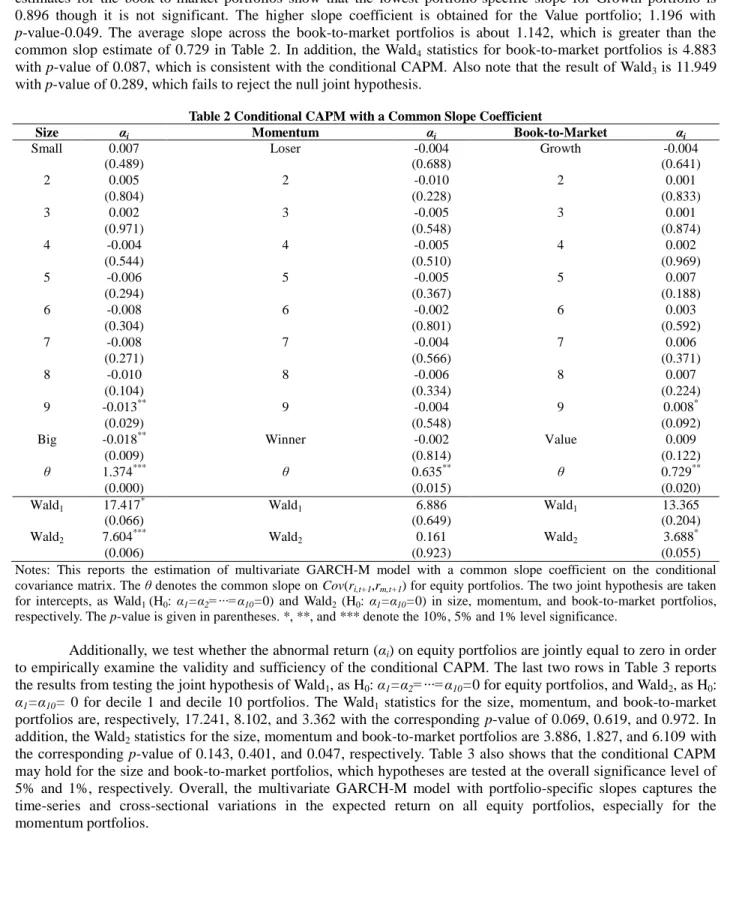
In this paper, by pooling a large number of time-series and cross-section together, we investigate the characterization of time-series variation in conditional covariance and capture the cross-sectional correlations among equity portfolios by means of multivariate GARH-M model with DCC. According to the conditional CAPM, the reward-to-risk coefficient should be restricted to be positive and significant. Table 2 presents the sign and significance of all three reward-to-risk coefficients give similar conclusions and reports the common slope coefficient (θ), the conditional alpha (αi), and the p-value of the parameter estimate for each equity portfolio. As shown in Table 2, the estimates of common slopes provide empirical support for the positive relationship between the expected return and risk in Chinese exchange markets. The estimated coefficients on Cov(ri,t+1,rm,t+1) are always positive and significant, i.e. θ=1.374 with significant p-value at zero for the size portfolios, θ=0.635 with the p-value at 0.015 for the momentum portfolios, and θ=0.729 with p-value at 0.020 for the book-to-market portfolios. Overall, these findings in DCC-based conditional covariation estimates predict the time-series and cross-sectional variation in stock returns and they generate significant and reasonable risk premium.

The conditional CAPM estimation with a portfolio-specific Slope Coefficient

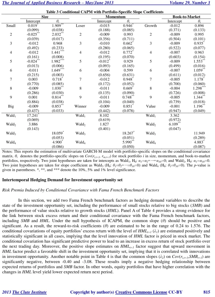
Table 3 presents the multivariate GARH-M model with portfolio-specific slopes based on ten size, momentum, and book-to-market portfolios, respectively. As it shown, all portfolio-specific coefficients on Cov(ri,t+1,rm,t+1) are estimated to be positive, though the significant level may vary among equity portfolios. For the size portfolios, the slope is the highest for the Small portfolio is 1.909 with p-value of 0.038, whereas the slope for the Big portfolio is 0.85 with p-value of 0.033. The average slope across the size portfolio is 1.340 that is close to the common slope estimate of 1.374 in Table 2. Furthermore, the Wald statistics from testing the joint hypothesis by Wald3 (H0: θ1=θ2=∙∙∙=θ10=0) and Wald4 (H0: θ1=θ10=0) are 18.059 with a p-value of 0.053 and 4.900 with a p-value of 0.086, respectively, supporting the cross-sectional consistency assumption of the conditional CAPM. In contrast to our earlier findings in Table 1, the results for the momentum portfolios show that the Loser portfolio that is composed of lowest return stocks has the highest portfolio-specific slope: 0.946 with p-value of 0.085, whereas the Winner portfolio that is composed of highest return stocks has a lower slope; 0.851 with p-value of 0.078. The average slope on momentum portfolios is 0.842, which is greater than the common slope estimate of 0.635 in Table 2. Moreover, the Wald3 and Wald4 statistics are 18.267 with p-value of 0.051 and 5.990 with a p-value of 0.050,

1

Examples of macro-level events that affect stock prices include sudden policy shifts by government to either stimulate or slow the economy, international trade disputes, and political crises.

respectively. Therefore, the result of momentum portfolios is also consistent with the conditional CAPM. The estimates for the book-to-market portfolios show that the lowest portfolio-specific slope for Growth portfolio is 0.896 though it is not significant. The higher slope coefficient is obtained for the Value portfolio; 1.196 with p-value-0.049. The average slope across the book-to-market portfolios is about 1.142, which is greater than the common slop estimate of 0.729 in Table 2. In addition, the Wald4 statistics for book-to-market portfolios is 4.883

with p-value of 0.087, which is consistent with the conditional CAPM. Also note that the result of Wald3 is 11.949

with p-value of 0.289, which fails to reject the null joint hypothesis.

Table 2 Conditional CAPM with a Common Slope Coefficient

Size αi Momentum αi Book-to-Market αi

Small 0.007 Loser -0.004 Growth -0.004

(0.489) (0.688) (0.641) 2 0.005 2 -0.010 2 0.001 (0.804) (0.228) (0.833) 3 0.002 3 -0.005 3 0.001 (0.971) (0.548) (0.874) 4 -0.004 4 -0.005 4 0.002 (0.544) (0.510) (0.969) 5 -0.006 5 -0.005 5 0.007 (0.294) (0.367) (0.188) 6 -0.008 6 -0.002 6 0.003 (0.304) (0.801) (0.592) 7 -0.008 7 -0.004 7 0.006 (0.271) (0.566) (0.371) 8 -0.010 8 -0.006 8 0.007 (0.104) (0.334) (0.224) 9 -0.013** 9 -0.004 9 0.008* (0.029) (0.548) (0.092)

Big -0.018** Winner -0.002 Value 0.009

(0.009) (0.814) (0.122)

θ 1.374*** _{θ 0.635}** _{θ 0.729}**

(0.000) (0.015) (0.020)

Wald1 17.417* Wald1 6.886 Wald1 13.365

(0.066) (0.649) (0.204) Wald2 7.604 *** Wald2 0.161 Wald2 3.688 * (0.006) (0.923) (0.055)

Notes: This reports the estimation of multivariate GARCH-M model with a common slope coefficient on the conditional covariance matrix. The θ denotes the common slope on Cov(ri,t+1,rm,t+1) for equity portfolios. The two joint hypothesis are taken

for intercepts, as Wald1 (H0: α1=α2=∙∙∙=α10=0) and Wald2 (H0: α1=α10=0) in size, momentum, and book-to-market portfolios,

respectively. The p-value is given in parentheses. *, **, and *** denote the 10%, 5% and 1% level significance.

Additionally, we test whether the abnormal return (αi) on equity portfolios are jointly equal to zero in order to empirically examine the validity and sufficiency of the conditional CAPM. The last two rows in Table 3 reports the results from testing the joint hypothesis of Wald1, as H0: α1=α2=∙∙∙=α10=0 for equity portfolios, and Wald2, as H0:

α1=α10= 0 for decile 1 and decile 10 portfolios. The Wald1 statistics for the size, momentum, and book-to-market

portfolios are, respectively, 17.241, 8.102, and 3.362 with the corresponding p-value of 0.069, 0.619, and 0.972. In addition, the Wald2 statistics for the size, momentum and book-to-market portfolios are 3.886, 1.827, and 6.109 with

the corresponding p-value of 0.143, 0.401, and 0.047, respectively. Table 3 also shows that the conditional CAPM may hold for the size and book-to-market portfolios, which hypotheses are tested at the overall significance level of 5% and 1%, respectively. Overall, the multivariate GARCH-M model with portfolio-specific slopes captures the time-series and cross-sectional variations in the expected return on all equity portfolios, especially for the momentum portfolios.

Table 3 Conditional CAPM with Portfolio-Specific Slope Coefficients

Size Momentum Book-to-Market

Intercept θi Intercept θi Intercept θi

Small 0.019* 1.909** Loser -0.015 0.946* Growth -0.012 0.896

(0.099) (0.038) (0.188) (0.085) (0.371) (0.133) 2 -0.025** 2.032** 2 -0.009 0.993 2 -0.009 0.995 (0.039) (0.017) (0.356) (0.711) (0.504) (0.101) 3 -0.012 0.968 3 -0.010 0.662* 3 -0.009 0.935* (0.492) (0.233) (0.280) (0.065) (0.522) (0.077) 4 -0.012 1.441*** 4 -0.012 0.772* 4 -0.007 0.963 (0.161) (0.008) (0.195) (0.070) (0.603) (0.154) 5 -0.024** 1.982*** 5 -0.012* 0.929 5 -0.009 1.553** (0.013) (0.006) (0.093) (0.165) (0.499) (0.016) 6 -0.011 1.649*** 6 -0.004 0.599 6 -0.007 1.059** (0.215) (0.003) (0.656) (0.631) (0.611) (0.012) 7 0.003 0.718* 7 -0.012 0.948* 7 -0.005 1.178* (0.770) (0.085) (0.172) (0.052) (0.700) (0.060) 8 -0.009 1.030** 8 -0.011 0.669* 8 -0.004 1.298*** (0.286) (0.030) (0.135) (0.090) (0.726) (0.008) 9 0.001 0.814** 9 -0.011 0.748** 9 -0.005 1.344** (0.884) (0.038) (0.104) (0.040) (0.739) (0.018)

Big -0.009 0.853** Winner -0.009 0.851* Value -0.001 1.196**

(0.437) (0.033) (0.442) (0.078) (0.947) (0.049)

Wald1 17.241* Wald1 8.102 Wald1 3.362

(0.069) (0.619) (0.972)

Wald2 3.886 Wald2 1.827 Wald2 6.109**

(0.143) (0.401) (0.047)

Wald3 18.059* Wald3 18.267* Wald3 11.949

(0.053) (0.051) (0.289)

Wald4 4.900* Wald4 5.990** Wald4 4.883*

(0.086) (0.050) (0.087)

Notes: This reports the estimation of multivariate GARCH-M model with portfolio-specific slopes on the conditional covariance matrix. θi denotes the portfolio-specific slopes on Cov(ri,t+1, rm,t+1) for stock portfolio i in size, momentum, and book-to-market

portfolios, respectively. Two joint hypotheses are taken for intercepts as Wald1, H0: α1=α2=∙∙∙=α10=0; and Wald2, H0: α1=α10=0.

Two joint hypotheses are taken for slope coefficient as Wald3 (H0: θ1=θ2=∙∙∙=θ10=0) and Wald4 (H0: θ1=θ10=0). The p-value is

given in parentheses. *, **, and *** denote the 10%, 5% and 1% level significance.

Intertemporal Hedging Demand for Investment opportunity set

Risk Premia Induced by Conditional Covariance with Fama French Benchmark Factors

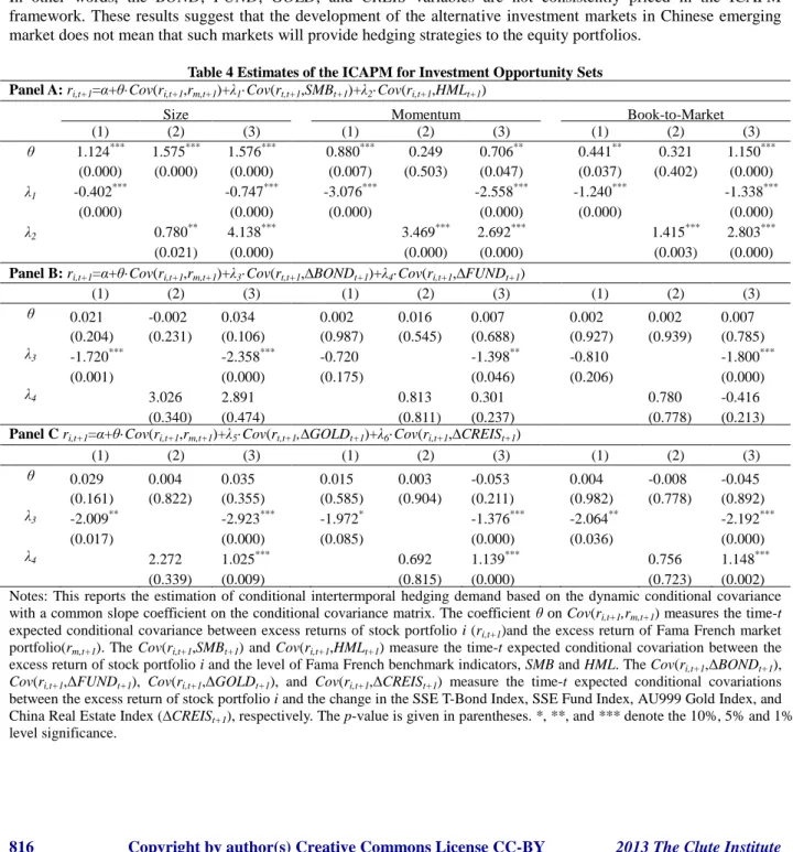
In this section, we add two Fama French benchmark factors as hedging demand variables to describe the state of the investment opportunity set, including the performance of small stocks relative to big stocks (SMB) and the performance of value stocks relative to growth stocks (HML). Panel A of Table 4 provides a strong evidence for the link between stock excess return and their conditional covariance with the Fama French benchmark factors, including SMB and HML. Under the null hypothesis of ICAPM, the common slope (θ) should be positive and significant. As a result, the reward-to-risk coefficients (θ) are estimated to be in the range of 0.24 to 1.576. The conditional covariations of equity portfolios’ excess return with the level of HMLt+1 (λ1) are estimated positively and statistically significant in all cases, implying that the level innovation of HML factor is priced in stock market. The conditional covariation has significant predictive power to lead to an increase in excess return of stock portfolio over the next trading day. Moreover, the positive slope estimates on HMLt+1 factor suggest that upward movement in HML factor predict a favorable shift in the investment opportunity set, implying that it is correlated with innovations in investment opportunity. Another notable point in Table 4 is that the common slopes (λ2) on Cov(ri,t+1,SMBt+1) are significantly negative, between -0.40 and -3.08. These results imply a negative hedging relationship between expected returns of portfolios and SMB factor. In other words, equity portfolios that have higher correlation with the changes in HML level yield lower expected return next period.

Risk Premia Induced by Conditional Covariance with Financial Instrument

Investors would pick the winning stocks in the exchange market if they had perfect foresight. But, there is no free lunch in the financial market. Indeed, it is most often that the market participants seek to hedge stock risk through alternative investments, and vice versa, the well-functioning hedging solutions are important to the needs of either domestic or international investors. Financial economists often choose certain market indicators to control for stochastic shifts in the investment opportunity set. Panel B and C in Table 4 present the measures of common slope coefficients on the covariance of each equity portfolio with four financial instruments. The common slope of the risk-return coefficients are estimated insignificantly to zero. The conditional covariance of the return of equity portfolio with financial instrument does not have robust power for size, momentum, and book-to-market portfolios. In other words, the BOND, FUND, GOLD, and CREIS variables are not consistently priced in the ICAPM framework. These results suggest that the development of the alternative investment markets in Chinese emerging market does not mean that such markets will provide hedging strategies to the equity portfolios.

Table 4 Estimates of the ICAPM for Investment Opportunity Sets Panel A: ri,t+1=α+θ·Cov(ri,t+1,rm,t+1)+λ1·Cov(rt,t+1,SMBt+1)+λ2·Cov(ri,t+1,HMLt+1)

Size Momentum Book-to-Market

(1) (2) (3) (1) (2) (3) (1) (2) (3) θ 1.124*** _1.575*** _1.576*** _0.880*** _{0.249 0.706}** _0.441** _{0.321 1.150}*** (0.000) (0.000) (0.000) (0.007) (0.503) (0.047) (0.037) (0.402) (0.000) λ1 -0.402*** -0.747*** -3.076*** -2.558*** -1.240*** -1.338*** (0.000) (0.000) (0.000) (0.000) (0.000) (0.000) λ2 0.780** 4.138*** 3.469*** 2.692*** 1.415*** 2.803*** (0.021) (0.000) (0.000) (0.000) (0.003) (0.000)

Panel B:ri,t+1=α+θ·Cov(ri,t+1,rm,t+1)+λ3·Cov(rt,t+1,∆BONDt+1)+λ4·Cov(ri,t+1,∆FUNDt+1)

(1) (2) (3) (1) (2) (3) (1) (2) (3) θ _{0.021 -0.002 0.034 0.002 0.016 0.007 0.002 0.002 0.007} (0.204) (0.231) (0.106) (0.987) (0.545) (0.688) (0.927) (0.939) (0.785) λ3 -1.720*** -2.358*** -0.720 -1.398** -0.810 -1.800*** (0.001) (0.000) (0.175) (0.046) (0.206) (0.000) λ4 3.026 2.891 0.813 0.301 0.780 -0.416 (0.340) (0.474) (0.811) (0.237) (0.778) (0.213)

Panel C ri,t+1=α+θ·Cov(ri,t+1,rm,t+1)+λ5·Cov(rt,t+1,∆GOLDt+1)+λ6·Cov(ri,t+1,∆CREISt+1)

(1) (2) (3) (1) (2) (3) (1) (2) (3) θ _{0.029 0.004 0.035 0.015 0.003 -0.053 0.004 -0.008 -0.045} (0.161) (0.822) (0.355) (0.585) (0.904) (0.211) (0.982) (0.778) (0.892) λ3 -2.009** -2.923*** -1.972* -1.376*** -2.064** -2.192*** (0.017) (0.000) (0.085) (0.000) (0.036) (0.000) λ4 2.272 1.025*** 0.692 1.139*** 0.756 1.148*** (0.339) (0.009) (0.815) (0.000) (0.723) (0.002)

Notes: This reports the estimation of conditional intertermporal hedging demand based on the dynamic conditional covariance with a common slope coefficient on the conditional covariance matrix. The coefficient θ on Cov(ri,t+1,rm,t+1) measures the time-t

expected conditional covariance between excess returns of stock portfolio i (ri,t+1)and the excess return of Fama French market

portfolio(rm,t+1). The Cov(ri,t+1,SMBt+1) and Cov(ri,t+1,HMLt+1) measure the time-t expected conditional covariation between the

excess return of stock portfolio i and the level of Fama French benchmark indicators, SMB and HML. The Cov(ri,t+1,ΔBONDt+1),

Cov(ri,t+1,ΔFUNDt+1), Cov(ri,t+1,ΔGOLDt+1), and Cov(ri,t+1,ΔCREISt+1) measure the time-t expected conditional covariations

between the excess return of stock portfolio i and the change in the SSE T-Bond Index, SSE Fund Index, AU999 Gold Index, and China Real Estate Index (∆CREISt+1), respectively. The p-value is given in parentheses. *, **, and *** denote the 10%, 5% and 1%

CONCLUSIONS

In this context, we estimate the monthly intertemporal relationship between the expected return and risk using three categories of equity portfolios in Chinese exchange market, including size, momentum, and book-to-market portfolios. By doing so, we not only obtain the cross-sectional consistency of estimated intertemporal relationship, but also gain the statistical power by pooling multiple time-series and cross-section together for a joint estimation with common slope coefficients. Our results provide evidence to support the validity and sufficiency of conditional CAPM with a common slope coefficient and indicate that the conditional measures of market risk show the predictive power for the time-series and cross-sectional variations in expected return on equity portfolios. Further investigation of intertemporal hedging demand suggest that the factor SMB play a significant role as an alternative investment vehicle in hedging against the changes for equity portfolios. However, incorporating the conditional covariations with any of alternative investment financial intruments is not consistently priced in the ICAPM framework. Further analysis therefore is required to seek hedging investments to protect against the emerging market risk.

AUTHOR INFORMATION

Zhongyi Xiao is a Ph.D student in Department of Economics at Texas Tech University, USA. He has interested in various areas of financial economics. E-mail: [email protected]

Peng Zhao is an Associate Professor of Management information system in School of Economics and Business Administration, Chongqing University, China. He is teaching courses on information management and data procession at both undergraduate and graduate level. E-mail: [email protected] (Corresponding author) REFERENCES

1. Backus, D.K., & Gregory, A. W. (1993). Theoretical relations between risk premiums and conditional variances. Journal of Business & Economic Statistics, 11(2), 177-185.

2. Bali, T. G. & Engle, R. F. (2010a). Resurrecting the conditional CAPM with dynamic conditional correlations. http://dx.doi.org/10.2139/ssrn.1298633

3. Bali, T. G. (2008). The intertemporal relation between expected returns and risk. Journal of Financial Economics,87(1), 101-131.

4. Bali, T. G. & Engle, R. F. (2010b). The intertemporal capital asset pricing model with dynamic conditional correlations. Journal of Monetary Economics, 57(4), 377-390.

5. Black, F. (1972). Capital market equilibrium with restricted borrowing. Journal of Business, 45(3), 444-455.

6. Brandt, M. W. & Kang, Q. (2004). On the relationship between the conditional mean and volatility of stock returns: A latent VAR approach. Journal of Financial Economics, 72(2), 217-257.

7. Buraschi, A., Porchia, P. & Trojani, F. (2010). Correlation risk and optimal portfolio choice. The Journal of Finance, 65(1), 393-420.

8. Campbell, R., Koedijk, K. & Kofman, P. (2002). Increased correlation in bear markets. Financial Analysts Journal, 58(1), 87-94.

9. Chauvet, M. & Potter, S. (2000). Coincident and leading indicators of the stock market. Journal of Empirical Finance,7(1), 87-111.

10. Engle, R. F. (2002). Dynamic conditional correlation. Journal of Business and Economic Statistics, 20(3), 339-350.

11. Fama, E. F. (1991). Efficient capital markets: II. The Journal of Finance,46(5), 1575-1617.

12. Fama, E. F. & French, K. R. (1992). The cross‐section of expected stock returns. The Journal of Finance, 47(2), 427-465.

13. Fama, E. F. & French, K. R. (1992). Value versus Growth: The International Evidence. The Journal of Finance, 53(6), 1975-1999.

14. Glosten, L. R., Jagannathan, R. & Runkle, D. E. (1993). On the relation between the expected value and the volatility of the nominal excess return on stocks. The Journal of Finance, 48(5), 1779-1801.

15. He, Z., Huh, S. W. & Lee, B. S. (2010). Dynamic factors and asset pricing. Journal of Financial and Quantitative Analysis, 45(3), 707.

16. Jegadeesh, N. & Titman, S. (1993). Returns to buying winners and selling losers: Implications for stock market efficiency. The Journal of Finance, 48(1), 65-91.

17. Lintner, J. (1965). The valuation of risk assets and the selection of risky investments in stock portfolios and capital budgets. The Review Of Economics and Statistics, 47(1), 13-37.

18. Newey, W. K., & Kenneth D. W. (1987). A Simple, Positive Semi-Definite, Heteroskedasticity and Autocorrelation Consistent Covariance Matrix, Econometrica, 55(3), 703–708.

19. Merton, R. C. (1973). An Intertemporal Capital Asset Pricing Model. Econometrica,41(5), 867-887. 20. Merton, R. C. (1980). On Estimating The Expected Return on The Market: An Exploratory Investigation.

Journal of Financial Economics, 8(4), 323-361.

21. Sharpe, W. F. (1964). Capital Asset Prices: A Theory Of Market Equilibrium Under Conditions Of Risk. The Journal of Finance, 19(3), 425-442.

22. Su, D. & Fleisher, B. M. (1998). Risk, Return, and Regulation in Chinese Stock Market. Journal of Econometric and Business, 50(3), 239-256

23. Sun, Q. & Tong, W. H. S. (2000). The Effect of Market Segmentation on Stock Prices: the China Syndrome. Journal of Banking and Finance, 24(12), 1875-1902.

24. Whitelaw, R. F. (1994). Time Variations and Covariations in the Expectation and Volatility of Stock Market Returns. The Journal of Finance, 49(2), 515-541.

25. Whitelaw, R. F. (2000). Stock Market Risk and Return: An Equilibrium Approach. Review of Financial Studies, 13(3), 521-547.

26. Xiao, Z., Zhao, P., Rahnama, M. & Zhou, Y. (2012). Winner versus Loser: Time-Varying Performance And Dynamic Conditional Correlation. Journal of Applied Business Research, 28(4), 581-594.