Mobility Models and User Adaptation Based Simulation

Extracting a mobility model from real user traces

Minkyong Kim

Dartmouth College Hanover, NH [email protected]

David Kotz

Dartmouth College Hanover, NH [email protected]

Songkuk Kim

Wilson Center for Research & Technology Xerox Corporation

Webster, NY [email protected]

Abstract— Understanding user mobility is critical for simula-tions of mobile devices in a wireless network, but current mobility models often do not reflect real user movements. In this paper, we provide a foundation for such work by exploring mobility characteristics in traces of mobile users. We present a method to estimate the physical location of users from a large trace of mobile devices associating with access points in a wireless network. Using this method, we extracted tracks of always-on Wi-Fi devices from a 13-month trace. We discovered that the speed and pause time each follow a log-normal distribution and that the direction of movements closely reflects the direction of roads and walkways. Based on the extracted mobility characteristics, we developed a mobility model, focusing on movements among popular regions. Our validation shows that synthetic tracks match real tracks with a median relative error of 17%.

I. INTRODUCTION

The purpose of mobile computing and communications is to allow people to move about and yet be able to interact with information, services, and other people. Anyone designing an application, system, or network to serve mobile users must therefore have some notion about how the users, and their devices, move. Indeed, most researchers use simulation to discover how their application, system or network responds to variations in user activity, including mobility. It is thus critical to support such simulations with a realistic model of user mobility—and yet, most mobility models used by this research community are ad hoc creations based on the intuition of their designer. Few models are derived from traces of real user behavior. The mobile and ad-hoc networks (MANET) community depends on simple but unrealistic variations of random-walk models, for example. An alternative to model-based simulation may be trace-driven simulation. Although trace-driven simulation does not require a mobility model, model-based simulation allows researchers to explore a larger parameter space.

To develop a mobility model, we must understand user mo-bility. We must obtain detailed mobility data about real users, and carefully characterize their mobility. This characterization provides useful insights itself, for example, to researchers interested in predicting mobility in support of location-aware applications [1] or for network optimization [2]. Recent re-search in opportunistic ad hoc networking also depends on an understanding of user mobility and the opportunities for user devices to interact when users pass close to each other. Some recent work [3] distributed portable devices to real people to

collect data about such opportunities, but these studies are based on small populations. One study [4] examines the large traces collected at Dartmouth College [5], [6] and UCSD [7], but only recognizes opportunities when the users are at the same Wi-Fi access point (AP), in contrast to when the users are within communication range of each other.

This paper describes our experiences in extracting user mo-bility characteristics from wireless network traces (syslog) and developing a mobility model based on these characteristics. We chose to use syslog traces because these traces are relatively easy to collect for large user populations; for example, the traces collected at Dartmouth College contain data from nearly 10,000 users over several years. Any wireless ISP provider also has access to similar data.

Although syslog traces are readily available, we cannot extract mobility characteristics directly from them. These traces contain sequences of access points with which wireless devices associated. From these sequences, we need to extract locations of users over time. We explored several methods to extract mobility tracks from syslog traces.

We also developed a heuristic to extract mobility charac-teristics from mobility tracks. From these traces we cannot know whether a user was moving or not, so we need a way to estimate pause durations. We validate this heuristic using the data collected by controlled walks and then apply the heuristic to our wireless network traces to collect mobility characteristics.

We analyzed mobility characteristics including pause time, speed, and direction of movements. We found that pause time and speed distributions each follow a log-normal distribution. Not surprisingly, the directions of movement do not follow a uniform distribution, although many MANET researchers make that assumption in their simulations. Instead, the di-rections of movement follow the direction of popular roads and walkways on the campus, and shows a strong symmetry across 180 degrees. These mobility characteristics provide the fundamental information that underlies any mobility model.

For our mobility model, we first define popular regions, hotspots, and characterize these regions. We concentrate on movements among hotspots, supposedly more interesting re-gions for many applications. Researchers who want to simulate how users aggregate (e.g., a friend-finder application [8]) need to have this type of model. Those who want to explore aspects of context-aware systems (such as scalability of context-aware

services [9]) can also benefit from such a model.

Finally, we use mobility characteristics to develop a soft-ware model that generates realistic user mobility tracks. We validate our model by comparing synthetic tracks with real tracks. Our validation shows that synthetic tracks match real tracks with a median relative error of 17%.

II. COLLECTING USER TRACES

We use the wireless network data set collected at Dartmouth College to derive mobility information. The Dartmouth trace data is the largest publicly-available set of Wi-Fi network traces, comprising syslog, SNMP and tcpdump data that has been collected since 2001 [5], [6]. In this paper, we concentrate on the syslog data collected from the beginning of June 2003 to the end of June 2004. At the time, the Dartmouth WLAN consisted of approximately 560 access points (the number of APs changes over time as the network evolves). Whenever clients authenticate, associate, roam, disassociate or deauthenticate with an AP, a syslog message is recorded, containing a timestamp in seconds, the client MAC address, the AP name and the event type. Note that syslog traces do not contain signal-strength information, which would have been useful for locating clients.

The Dartmouth trace data includes a map, indicating the

(x, y, z)coordinate of most of the APs on campus. We define a location as a pair of (x, y) coordinates on the map. (We ignore the z coordinate, an integer representing the building floor on which the AP is located, in our study; we hope to extend our approach to three dimensions in future work.) If a map of access points is not available, one can collect

location of APs through methods such as war-driving (as

used by Place Lab [10], [11]), or using AP position-estimation techniques [12].

For the purposes of characterizing mobility, we are only interested in a subset of wireless network users: the Voice-over-IP (VoIP) device users. Most of the Dartmouth wireless network clients are laptop users, but most of these clients are not very mobile, or are nomadic in their mobile network usage. We chose to concentrate on the always-on VoIP device users, as these have been shown to have higher mobility [5]. We obtained a list of 198 MAC addresses belonging to Cisco 7920 Wi-Fi VoIP telephones and Vocera VoIP communicators, and only considered syslog data containing one of these MAC addresses.

For each VoIP-client MAC address in the trace data, we extracted the syslog events for each day. To remove diurnal effects where a client will be less mobile at night (for instance, where the owner of a VoIP device goes home off-campus at night but leaves the device charging in their office), we only consider the working day by ignoring any events before 8 AM and after 6 PM on each day.

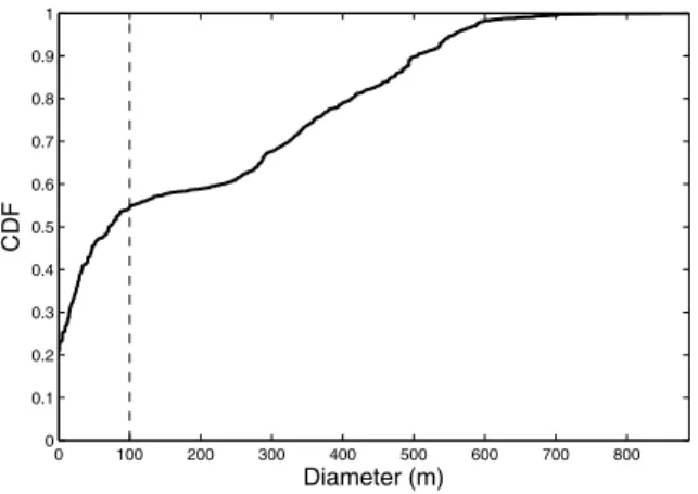
We then divided the workday traces into stationary and mo-bile sets. For each workday’s trace, we calculated itsdiameter: the maximum Euclidean distance between the locations of any two APs that a user visits on that workday. Figure 1 shows the cumulative distribution function (CDF) of diameter for 7,128

0 100 200 300 400 500 600 700 800 0 0.1 0.2 0.3 0.4 0.5 0.6 0.7 0.8 0.9 1 Diameter (m) CDF

Fig. 1. Diameter. CDF of diameter across 7,128 workdays. The diameter of 100 m (denoted by the dotted vertical line) is used as the cutoff to separate workday traces into stationary and mobile sets.

Mobile Stationary (≥100m) (<100m) Total Cisco 681 (34%) 1,330 2,011 Vocera 2,571 (50%) 2,546 5,117 Total 3,252 (46%) 3,876 7,128 TABLE I

WORKDAY TRACE SUMMARY.THIS TABLE SHOWS THE NUMBER OF TRACES FOR MOBILE AND STATIONARY SETS.

workdays. The CDF shows a plateau starting approximately at 100 m. Thus, we used 100 m as our cutoff (shown as the dotted vertical line) to distinguish between the stationary set of workdays and the mobile set. Workdays that have a diameter of less than 100 m are considered stationary, while all other workdays are considered mobile. Table I shows the number of workdays in the stationary and mobile sets. 46% of all workdays are considered mobile.

We parsed these syslog traces to obtain mobility traces. A mobility trace lists locations of APs with which the device associated, authenticated, or roamed along with a timestamp for each action. (In the text that follows,associationrefers to all three types of actions.) The parser also separates a workday of a device into multiple walks whenever the device was off for more than thirty minutes. We detected these “off” states using the deauthenticate message that an AP generates for a client who has not sent any message for the past thirty minutes. The 3,252 mobile traces are converted to 3,838 walks, and the 3,876 stationary traces are converted to 4,006 walks.

III. TRACE PROCESSING ALGORITHMS

From these mobility traces, we need to extract user locations or usertracks. Since we cannot tell, from these traces, whether a user moved or not at a particular time, we also need to estimate pause duration.

A. Estimating user tracks

The mobility traces provide the sequence of coordinates of APs for each user on each workday, but line segments connecting these coordinates in sequence may be far from the user’s geographical location over time. While it is possible

GPS track APs

Fig. 2. AP associations.A pedestrian carried a Vocera communicator on an outdoor walk around campus. This figure shows line segments between APs the Vocera associated in sequence.

to estimate the location of a Wi-Fi user by having its client sense multiple nearby APs (as with Place Lab [10] and many others), it is experimentally difficult to obtain such location traces from thousands of users. In contrast, syslog data, which is recorded by the AP, is readily available. Thus, we explore methods to estimate user locations from syslog data.

There are several reasons that locations in syslog data may be different from a user’s location. First, most users do not stand next to an AP, and then walk to a point next to another AP. Second, mobile devices do not necessarily associate with the geographically-closest AP. This behavior results from many reasons, such as different APs being con-figured with different power levels, or the signal from close APs being blocked by buildings or trees. Third, different devices have different aggressiveness in changing associations. Less-aggressive devices do not change the associated AP as frequently. Thus, they may be associated with an AP far from the user’s current location.

To get a sense of how VoIP devices change associations, we asked a volunteer to walk around on the Dartmouth campus with a GPS device and a Vocera communicator. After registering the GPS data to the AP map coordinates, we plotted the actual path (according to GPS) and the associations in the same figure. Figure 2 shows both the GPS track and the crude track of a user’s location by drawing line segments between the map coordinates of APs in sequence; the arrow shows the direction of the walk. Clearly, a mobile user roams widely from AP to AP. This crude method estimates a mobility track that is far from the GPS track.

Based on the above observations, we need a method to estimate a smooth path representing the user’s location over time. We explore three approaches to address this problem.

1) Triangle centroid: The centroid algorithm uses location of past three AP associations as the vertices of a triangle. We estimate the user’s location as the centroid of a triangle, which is the intersection of the triangle’s three triangle medians. The location estimate is updated whenever there is an association message.

2) Time-based centroid: Because devices do not change

associations periodically, using the past three associations may be ineffective, especially for less aggressive devices. Thus, we explore the centroid algorithm with a window of a fixed-time period,q. Everypseconds, we update the user’s location with associations that happened during the pastqseconds. Thus, a user’s location at timet is defined as:

¯

x(t) =_n1n_i=1xi, y¯(t) =_n1n_i=1yi (1)

where n is the number of associations within the past q

seconds. If there has been no association within the past q

seconds (n= 0), we keep the previous location estimate:

¯

x(t) = ¯x(t−p), y¯(t) = ¯y(t−p). (2)

The default values for p and q are 10 and 60 seconds,

respectively. Note thatnchanges dynamically for each update for this method, while n is fixed at three for the triangle centroid algorithm.

3) Kalman filter: A Kalman filter is a recursive data pro-cessing algorithm that produces optimal estimates. While this filter requires significant knowledge of the system, one can make reasonable guesses to get a good result.

The system to be estimated can be modeled as:

xk+1=Φkxk+wk (3)

where x_k represents the state of the system, Φ is a matrix relating one state x_k to the next state x_k+1, and w is a vector representing system noise. Our state variables include the user’s location (xandy) and velocity (x and y). Then, Equation 3 is written as:

    x x y y     k+1 =     1 t 0 0 0 1 0 0 0 0 1 t 0 0 0 1     k     x x y y     k +     w1 w2 w3 w4     k (4)

where tis the time difference between two consecutive asso-ciations.

The measurement of the system is defined as:

zk =Hkxk+vk (5)

where H is a matrix relating the state variables xk to the measurementszk, andvis a vector representing measurement error. For each associationk, we have the location of the AP with which a user is associated. Given this measurement, we update our estimate of the user’s location. Since the measured location can be considered as the user’s true location disturbed by some noise, Equation 5 can be written as:

z1 z2 _k= 1 0 0 0 0 0 1 0 _k     x x y y     k + v1 v2 _k. (6)

We now need to define the covariance matrices for w_k

and v_k, Q_k and R_k, respectively. Q represents the degree of variability in the state variables;Rrepresents the measure-ment uncertainty. Since the relationship between variances is

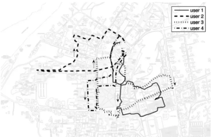
Fig. 3. GPS tracks.This figure shows the GPS tracks of four walks depicted on the Dartmouth campus map.

unknown, we assume that the variances are independent of each other, making their products zero. The resulting Qand R are: Qk =     w12 0 0 0 0 w22 0 0 0 0 w32 0 0 0 0 w42     Rk = v12 0 0 v22

Since it is the relative magnitude of values in covariance matrices that affects the filter’s performance, we set values in Qto one and empirically chose values forRin the following section.

4) Validation: To validate path extractors, we walked

around on the Dartmouth campus with a GPS device, a Vocera VoIP communicator, and a Cisco VoIP phone. GPS data serves as the ground truth and VoIP data is used to estimate a user’s path. We have data for four such walks, each made by a different person along a different path. Each walk lasted around 30 minutes, roughly 20 minutes walking and 10 minutes pausing at an indoor location. With these four walks, we were able to visit much of the area covered by the campus-wireless network. Figure 3 shows the GPS tracks of these walks on our campus map.

To get the difference between the tracks and GPS data, we computed the distance between the two every 30 seconds. Since there is no GPS data when a user was indoors, we excluded these time periods from the calculation. (These pause-time periods are later used to test our characterization technique.) Figure 4 illustrates the distance between a GPS track and an estimated track of a Vocera communicator for one of our walks.

Choosing Kalman parameters: We used all four walks to

choose the Kalman parameters. Since movements in xandy

directions are likely to be symmetric, we assume that errors in the xand y directions are same. Then, we have only one unknown variable, v2.

Fig. 4. Differences.This figure shows the difference between the GPS track and the path estimated using a Kalman filter.

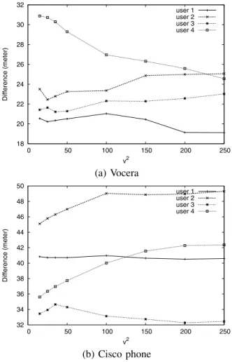
Figure 5 shows the median difference between the GPS track and the path estimated by Kalman filters with different

v2 values: 15, 25, 35, 50, 100, 150, 200, and 250. All users, except User 4, do not show a trend over different values of

v2. For User 4, as v2 increases, the difference decreases for the Vocera while it increases for the Cisco phone; there is not one good value for both. Thus, we chose 25 forv2 based on the local minimum observed for some of the Vocera users.

Evaluating path extractors: From our walks, we found that different types of devices have different association patterns. Vocera communicators aggressively associated with many APs, while the Cisco phones tended to stay associated with a single AP for a long time. Path extractors should be able to cope with these differences. We also observed that the distance from a device to the associated AP varies by a large amount; while a device tends to associate with nearby APs, it sometimes associated with APs as far as 200 meters away. Path extractors should be able to produce estimates with a bounded error range by coping with associations with far-away APs.

Figure 6 shows the difference result for Vocera commu-nicators and Cisco phones; each line shows the median and maximum of differences (measured every 30 seconds) for each user. The triangle centroid, time-based centroid, and Kalman filter are labeled as ‘triangle’, ‘time’, and ‘kalman’, respectively. In addition to these three algorithms, we included a crude track by connecting the locations of APs (like that shown in Figure 2); this track is labeled as ‘ap’.

The triangle-centroid algorithm produces relatively well-bounded estimates for Vocera communicators, but its medians for Cisco phones are much worse than the crude tracks. This result happens because Cisco phones tend to stay associated with an AP for a while, so using the past three associations is too slow to reflect a user’s current location. The time-based centroid algorithm works better than the triangle-centroid algorithm for Cisco phones, but it sometimes updates the user’s location with far-away APs as happened for Vocera User 2 and User 4. The Kalman filter produces estimates that are well bounded for Vocera communicators and it also works reasonably well for Cisco phones.

18 20 22 24 26 28 30 32 0 50 100 150 200 250 Difference (meter) v2 user 1 user 2 user 3 user 4 (a) Vocera 32 34 36 38 40 42 44 46 48 50 0 50 100 150 200 250 Difference (meter) v2 user 1 user 2 user 3 user 4 (b) Cisco phone

Fig. 5. Kalman parameter.This figure shows the median difference between the GPS track and the estimated path with differentv2values.

B. Extracting pause time

We then used the Kalman filter to extract user tracks, which are sequences of a user’s locations with timestamps indicating when the user arrived at each location. To characterize user mobility, we need to separate the time between two consec-utive associations into travel time and pause time. Since we cannot tell whether a user was moving by looking at the traces, we need to estimate pause duration.

1) Algorithm: We estimate pause duration using the user’s speed. If the speed between two locations is within a “normal” range, we assume that the user did not pause at the source location. If the speed is too slow, we assume that the user did not move at that slow speed, but instead, paused at the source before moving to the destination. When considering a “normal” range, we assume that users are pedestrians. This assumption is reasonable for the Dartmouth campus; most people walk rather than drive a car or take a bus on the campus because the campus is small. For an environment where users change their mode of transportation, we can adapt methods that detect mode of transit [13], [14].

Our track traces consists of an arrival time ti and location li, defined as (xi,yi). When a user arrives atli+1atti+1, the

1 2 3 4 0 20 40 60 80 100 120 140 160 180 200 User Difference (meter) ap triangle time kalman (a) Vocera 1 2 3 4 0 20 40 60 80 100 120 140 160 180 200 User Difference (meter) ap triangle time kalman (b) Cisco phone

Fig. 6. Path extractorsThis figure shows median(‘x’) and maximum(‘o’) of differences for Vocera communicators and Cisco phones.

speed froml_i to the new location l_i+1 is computed as

si= di

ei (7)

wherediis the Euclidean distance betweenl_iandl_i+1, andei

is the elapsed time,ti+1−ti. Ifsi is within the normal range, we assume that the user did not pause atl_i. We defined the normal range to bemin≤si≤10m/s; we explored different values ofmin: 0.1 m/s and 0.5 m/s. Ifsiis smaller thanmin, the user is likely to have paused atli before moving toli+1. Thus, bigger min values are likely to produce more pauses. The elapsed time, ei, is the sum of the pause time, pi, and the duration of travel,qi, as illustrated in Figure 7. The pause time,pi is computed as

pi =ei−qi=ei−di

s_i (8)

where si is the average speed of the user, computed as

expo-nentially weighted moving average: si= 0.25si+ 0.75si−1. In the traces we sometimes observe slow speeds due to pauses, but we also observe some high speeds. These high

speeds are observed only with short ei (a few seconds).

PAUSE DURATION

ASSOC_AP2

TIME

ASSOC_AP1 LEAVE_AP1

AP1 AP2

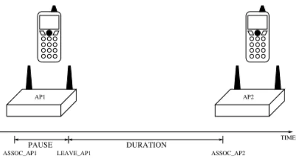
Fig. 7. Estimating pause and duration time.Assume a client moves from AP1 to AP2. Our data set only contains the association times ASSOC AP1 and ASSOC AP2. The user, however, may have paused at AP1, and so we need to estimate the pause time and the duration that it takes to travel from AP1 to AP2. recorded no clustering 15 m 35 m 55 m vocera 1 600 45; 598+20 45; 598+20 45; 618 45; 618 2 608 259+306 259+306 564 564 3 620 9; 632 9; 632 9; 632 9; 632 4 606 24; 677 24; 677 24; 677 24; 677 phone 1 600 38; 68+513 37; 68+513 38; 581 38; 581 2 608 569 569 569 569 3 620 646 646 646 646 4 606 86+79+258+34+144 603 603 603 TABLE II

PAUSE TIME OF FOUR USERS(UNIT:SECOND).THE EFFECT OF DIFFERENT CLUSTERING RANGES ON THE PAUSE-TIME COMPUTATION.

PAUSES AT THE PRE-DEFINED PAUSE LOCATIONS AND AT OTHER LOCATIONS ARE CONCENTRATED WITH‘+’AND‘;’,RESPECTIVELY.

Short ei is due to aggressive devices that change associations in searching for better signal reception. Thus, these high speeds are not likely to reflect a real movement of a user.

If si is greater than 10 m/s, we ignore the corresponding

segment when computing pause times pi and updating the

average speed si.

At the first movement between two locations in a track, we have no value for s_i, as we consider each track to be independent. In this case, we use a default speed value of 1.34 m/s (3 mile/h) as this is an average human walking speed. Note that the default value is used only when the first movement is out of the normal range.

The Kalman filter updates a user’s location whenever there is an association. Because a device can change associations even the user is not moving, the difference between consec-utive location estimates may be small. In this case, we want to aggregate the user’s pause time. Whenever a device pauses, we aggregate following pauses if those locations are within a fixed range from one another. We explore the effect of different “clustering ranges” in the following section.

With pause time defined for theith movement, we can now compute the speed of the user’s movement after the pause:

vi= di

ei−pi (9)

2) Validation: To validate our algorithm, we use the same four walks described earlier. We asked people to pause around

10 minutes at an indoor location during a 30-minute walk. Table II shows the pause time recorded by individuals and the time computed using our algorithm with different clustering ranges; the unit of time is second. For a given user, the recorded pause duration was same for both the Vocera and the phone. Note that our algorithm sometimes identified more than one pause. Pauses at the pre-defined pause locations are concentrated with ‘+’, while pauses at other locations are con-catenated with ‘;’. Smaller clustering ranges (no clustering and 15 meters) sometimes divided the 10-minute pause into several short ones. Bigger clustering ranges successfully aggregated short pauses into a long 10-minute pause. After 35 m, the result did not change. Thus, we chose 35 m as our clustering range. A clustering range that is too big may erroneously aggregate other short pauses (those separated by ‘;’ in the table) with the 10-minute pause. After clustering with a range of 35 m, the difference between the recorded time and the computed time for the 10-minute pause ranges from 3 seconds to 71 seconds. For some users, we have short pauses that happened at a location other than the 10-minute pause location. Some of these pauses may be errors while others turned out to be actual pauses. User 1 stopped momentarily before crossing a road; the pause locations for 45 seconds for the Vocera and 38 seconds for the Cisco phone match with the crossing point. C. Extracting hotspot regions

In addition to individual user’s mobility characteristics, we are also interested in identifying the popular locations. To define the regions that correspond to hotspots, we need to aggregate user destinations to determine the most popular destinations, that is, those destinations where the people spend the most time. One simple approach is to divide the area into fixed-sized regions and add the times that visitors spent in each region. One problem with this approach is that a highly popular hotspot may be divided into several regions and end up as a group of less popular spots. A further problem is that it is hard to determine an appropriate size for the unit region. Making it too small results in generating too many spots and not effectively aggregating visits, while making it too big results in generating over-sized hotspots. To avoid these problems, we chose not to divide our area into grid of fixed-sized regions.

Instead, we apply a 2-D Gaussian distribution to each pause location, weighted by duration of pause, and sum up the distri-bution. At each pause location, the 2-D Gaussian distribution creates a small ‘mountain’, uniformly distributed about its vertical axis. We add the ‘mountains’ for visits and consider those regions that are higher than a given threshold to be hotspots. We explore different threshold values in Section V-A. To select the appropriate Gaussian distribution, we need to define the standard deviation, σ. This σ should reflect the confidence in the exact user locations and the aggressiveness

in aggregating pauses. We chose σ of 20 meters based on

the result of our GPS experiment shown in Figure 6(a); the medians of the differences are close to this value.

102 103 104 10−4 10−3 10−2 10−1 100 Pause (s) CCDF

min=0.1m/s, not clustered min=0.1m/s, clustered min=0.5m/s, not clustered min=0.5m/s, clustered

Fig. 8. Pause.This figure shows the overall pause-time distribution.

IV. MOBILITY CHARACTERISTICS

Having verified that the Kalman filter provides a reasonable approximation of the GPS data, we apply this filter to the 3,838 mobile walks to produce the same number of mobility tracks. We then apply our pause-time estimator and extract mobility characteristics: pause time, speed, direction, start time, and end time.

For the 4,006 stationary walks, we do not extract user tracks. We estimate each user’s stationary location using the simple triangle centroid (Section III-A.1). We extract characteristics such as duration of stay, start time, and end time.

A. Mobile set

For both pause time and speed characterization, we use the complementary cumulative distribution function (CCDF):

F(x) = P(X ≥ x). CCDF is commonly drawn on a

logarithmic scale for both axes. The log-log CCDF helps determine whether a set of data fits a power law or heavy-tailed distribution; if the data is linear on a log-log scale, then this means that the data fits a power-law distribution.

Figure 8 shows the log-log CCDF of the number of pauses observed across all 3,838 walks as a function of pause duration in seconds. We explored two different values of min, used for our pause-time estimator (see Section III-B.1). Note that we only counted non-zero pauses. This figure shows the distributions of pauses both before and after clustering, using the clustering range of 35 meters (based on the validation presented in Section III-B.2). As expected, there were more

longer pauses when clustered. min of 0.5 m/s produced

relatively more shorter pauses than min of 0.1 m/s; this is because bigger min identifies more pauses. It is clear that none of distributions are linear. Using maximum likelihood estimation (MLE), we find that the clustered pauses fit a log-normal distribution, with a small number of users pausing for long periods of time.

Figure 9 shows the weighted log-log CCDF of the total duration of travel as a function of speed in meters per second. It includes distributions withminof 0.1 m/s and 0.5 m/s. The

10−1 100 101 10−4 10−3 10−2 10−1 100 Speed (m/s) CCDF min=0.1m/s min=0.5m/s

Fig. 9. Speed.This figure shows the overall speed distribution. The speed of each movement segment is weighted by duration of that movement.

0.01 0.02 0.03 0.04 30 210 60 240 90 270 120 300 150 330 180 0

Fig. 10. Direction.This figure shows a weighted PDF of movement direction with a bin size of 5°. The direction of each movement segment is weighted by duration of that movement.

speed of each movement segment is weighted by the duration of that movement.minof 0.5 m/s produced more faster speeds

than min of 0.1 m/s. The median for min of 0.5 m/s and

0.1 m/s are 0.43 m/s and 1.26 m/s, respectively; 1.26 m/s (2.8 mile/h) is close to the average human walking speed (3 mile/h). MLE finds that speed fits a log-normal distribution. Figure 10 shows the probability density function (PDF) of movement directions. The direction of each movement is weighted by the duration of that movement. The bin size is 5°. By manual comparison to a map of the Dartmouth campus, we found that the directions with larger peaks correspond to the directions of popular roads. Interestingly, the trends are repeated every 180°. We expect that this symmetry is because on a given road, people move in both directions. For instance, on a road that goes south and north, people move either northward or southward, generating peaks at two directions that are exactly 180° apart. Because of this symmetry, both the mean and median of the distribution are close to 0°.

Figure 11 shows a CDF of the start time and end time of each of 3,252 mobile workday traces. The line ‘start’ shows

8 9 10 11 12 13 14 15 16 17 18 0 0.1 0.2 0.3 0.4 0.5 0.6 0.7 0.8 0.9 1 Hour CDF start end

Fig. 11. Start and end times of mobile workdays.This figure shows the CDF across 3,219 workdays. ‘start’ denotes the time that devices first appeared within a workday; ‘end’ shows the time that devices disappeared.

Fig. 12. Mobile users on map.

the time that devices first appeared within a workday. The line ‘end’ shows the time that devices disappeared. Note that our chosen workday runs from 08:00 to 18:00; earlier start times were recorded as 08:00 and later end times as 18:00. 47% of workdays started by 09:00, and 53% ended after 17:00.

Figure 12 shows the distribution of pauses over our campus after applying a Gaussian distribution for each visit and adding them up. The darker spots represent higher mountains. The popular regions include the main Dartmouth library, the Department of Computer Science, the School of Engineering, the building with offices of network administrators, a hotel restaurant, and a gym.

B. Stationary set

We computed the duration of the stay for each of 4,006 walks. The duration of a walk is the difference between the time when the first and last messages of that walk were recorded. When there is only one message, the duration is zero. Note that this duration is an approximation of the time that a device was connected to the network. Since APs do not always generate deauthentication messages, which show the time that clients deauthenticate, we cannot rely on these messages to determine when clients went off. For example,

0 1 2 3 4 5 6 7 8 9 10 0 0.1 0.2 0.3 0.4 0.5 0.6 0.7 0.8 0.9 1 Duration (hour) CDF

Fig. 13. Duration of stay.The CDF of overall duration of stay across 4,006 stationary walks. The vertical dotted line shows the thirty-minute timeout used by APs to deauthenticate clients with no activities.

8 9 10 11 12 13 14 15 16 17 18 0 0.1 0.2 0.3 0.4 0.5 0.6 0.7 0.8 0.9 1 Hour CDF start end

Fig. 14. Start and end times of stationary workdays.This figure shows the CDF across 3,876 workdays. ‘start’ and ’end’ denote the time that devices first appeared and the time that devices disappeared within a workday.

if a device associates with an AP and no deauthentication message was generated, the computed duration for that device may be much shorter than the actual duration that the device was connected to the network.

Figure 13 shows the CDF of duration for 4,006 walks. About 29% had a duration of less than two minutes. The jump at thirty minutes is due to the fact that a client is deauthenticated if it has not sent any message for thirty minutes. After the thirty minute jump, the number of walks for different durations does not change much.

Figure 14 shows the CDF of start and end time for 3,876 stationary workdays. 28% of workdays started by 09:00 and 34% ended after 17:00. Compared to mobile workdays, sta-tionary workdays started later and ended earlier. This result may be because workdays that start later and end earlier are more likely to have small diameters, and thus are classified as stationary.

Figure 15 shows the users’ locations on the campus map after applying a Gaussian distribution for each stationary location. For this set of walks, we used the triangle centroid to

Fig. 15. Stationary users on map.The arrow denotes a popular region that is unique to stationary users.

compute the stationary location for each walk and calculated the number of walks at each location. Note that we did not consider the duration of stay for this set; each stationary lo-cation is weighted equally. Compared to the popular lolo-cations for mobile users (shown in Figure 12), the popular stationary locations are restricted to smaller regions. Nonetheless, these popular locations for stationary users coincide with those for mobile users. The only location that is unique for the stationary users is one of the clusters of undergraduate dorms, denoted by an arrow in Figure 15. The locations that were popular among mobile users, but not among stationary users, include a gym and a hotel containing a restaurant.

C. Summary of characteristics

Table III shows the summary of mobility characteristics. For each characteristic, we list the mean and median. The last two columns show the parameters for fitted distributions and the root mean square (RMS) error. Most characteristics are fitted as either log-normal distribution or exponential distribution. The equation for the PDF of the log-normal distribution is

f(x) = e−(ln(_xσx−√µ)2)/2σ2

2π , and that of the exponential

distri-bution is f(x) = eax+b. To fit data to a distribution, we first separated them into 100 bins. To remove the effect of truncating traces to working hours, we ignored the first bin for the start time, and ignored the last bin for the end time. The start and end time of both mobile and stationary sets follow exponential distributions. The pause times and speed of the mobile set follow log-normal distributions. The durations of the stationary set follow a uniform distribution.

V. CHARACTERIZING HOTSPOTS

The research community is often more interested in pop-ular regions, hotspots, where wireless users spend most of their time. For example, researchers working in opportunistic networking or developing context-aware services need to have an accurate model of these regions. Thus, we focus on these hotspots in developing a mobility model. We first define hotspot regions using a Gaussian distribution; the area outside of hotspots becomes the cold region. We then characterize each region separately.

4 5 6 7 8 9 10 11 1600 1800 2000 2200 2400 Number of hotspots Threshold

Fig. 16. Threshold for hotspots

A. Defining hotspot regions

Given the map of user destinations (Figures 12 and 15), we need to define hotspot regions by applying a threshold. Threshold values that are too low may generate too many or big regions as hotspots. Some of these hotspots may be in fact not popular locations. On the other hand, if the threshold value is too high, we may also select too many hotspots, as the threshold may divide a large region into several smaller hotspots.

To observe the effect of selecting different threshold values, we calculated the number of hotspots generated by varying the threshold from 1500 to 2500 in increments of 100. Figure 16 shows the result. Among the values that generated the mini-mum number of hotspots we chose the smallest, 1900; smaller values produce larger hotspots.

Figure 17 shows the regions represented by these five hotspots on a map of the Dartmouth campus. These hotspots coincide with the locations of several buildings popular among Vocera and Cisco phone users: the School of Engineering, the main Dartmouth library, the Computer Science department, the building with offices of campus network administrators, and a hotel containing a restaurant. Note that these hotspots represent popular spots among VoIP device users and may be different from popular spots of the whole Dartmouth population. B. Hotspot characteristics

Figure 18 shows a PDF of the number of users (walks) starting their day at each region (shown as black bars). The region labeled as ‘0’ represents tracks that started outside any hotspot (the cold region); the rest represents values for each hotspot. This figure also shows the area of each hotspot region normalized by the total area of all hotspots (shown as white bars). The size of the cold region is not included because we do not have a clear boundary of the campus and thus do not know the exact size of the cold region. Clearly, we see that the number of users and the hotspot size follow a similar trend, perhaps because a popular hotspot builds a larger ‘mountain’ with a larger base.

set characteristic unit mean median distribution RMS mobile start hour 1.9 (09:54) 1.1 (09:06) exponential a=−0.438 b=−0.872 0.5399

end hour 8.5 (16:30) 9.1 (17:06) exponential a= 0.523 b=−6.637 0.1844 pause (min=0.1m/s) hour 0.718 0.223 log-normal µ=−1.880 σ2= 5.085 1.1654 pause (min=0.5m/s) hour 0.466 0.045 log-normal µ=−2.700 σ2= 4.738 3.0781 speed (min=0.1m/s) m/s 0.76 0.43 log-normal µ=−0.741 σ2= 0.788 0.5252 speed (min=0.5m/s) m/s 1.64 1.26 log-normal µ= 0.290 σ2= 0.604 0.5253

direction degree -6.2° 2.5° -

-stationary start hour 3.3 (11:18) 2.4 (10:24) exponential a=−0.175 b=−1.599 0.3754 end hour 7.3 (15:18) 8.4 (16:24) exponential a= 0.249 b=−3.858 0.5246 duration (after 30 minutes) hour 5.1 5.0 uniform f(x) = 0.1055 0.3802

TABLE III

SUMMARY OF MOBILITY CHARACTERISTICS.

Fig. 17. Hotspots on campus map.This shows the hotspots identified with the threshold of 1900. Hotspots 1 to 5, in order, correspond to a hotel, the School of Engineering, the main Dartmouth library, the Computer Science department, and the building with offices of campus network administrators.

0 1 2 3 4 5 0 0.05 0.1 0.15 0.2 0.25 0.3 0.35 0.4 Region Probability Initial users Hotspot size

Fig. 18. Initial regions.This figure shows the initial region distribution of the number of users for each region. ‘0’ represents regions outside of five hotspots.

region. Figure 19 shows CDFs of pause time for five hotspots and the cold region. We first aggregated pause time as long as a user remains within the same region. The aggregated pause time depicts the duration of a user’s stay after entering a region. For each region, we have a CDF of the number of aggregated pauses for all walks as a function of aggregated pause duration. We include pause times of zero seconds; we need this information for simulation to decide whether to pause or not before moving to the next location. Figure 19 shows that the cold region has relatively more short pauses than any of the hotspots. This result is expected since we chose hotspots

0 0.5 1 1.5 2 2.5 3 3.5 x 104 0 0.1 0.2 0.3 0.4 0.5 0.6 0.7 0.8 0.9 1 Pause (s) CDF cold hot 1 hot 2 hot 3 hot 4 hot 5

Fig. 19. Pause distribution per region.This figure shows the CDF of pause time for five hotspots and the cold region.

as regions that have longer total pause times. Among the five hotspots, hotspot 2 and 3 have more long pauses. This implies that people tend to stay for a long time in these two regions: the School of Engineering and the main Dartmouth library.

To capture movements between different regions, we com-puted the probability of moving from one region to another. In addition to five hotspots and the cold region, we also defined theOFFstate. Thus, we have ann×ntransition matrix where

n−2 is the number of hotspots.

Among these seven states, the cold region is treated differ-ently. It is considered not as a destination, but as a waypoint that a user goes through or stops on the way from one hotspot to another. A waypoint is location li in our track traces described in Section III-B.1. For each transition from

one hotspot to another hotspot or OFF state, we count the

number of waypoints from traces, and generate a (n−1)×

(n−1) waypoint matrix that consists of the average number of waypoints when users moved between two regions.

VI. MODELING MOBILITY

We generate synthetic mobility tracks using our model and then compare these tracks to the real tracks, using character-istics that were not considered by the model.

A. Generating tracks

To simulate users’ movements, we use the following mo-bility characteristics that we described earlier:

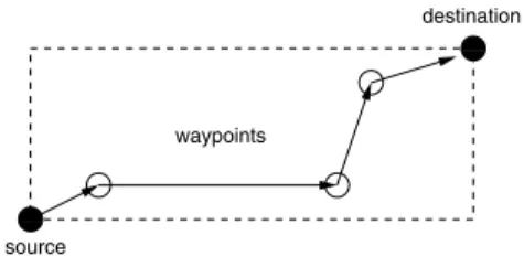
0 0 0 1 1 1 0 0 1 1 source waypoints destination

Fig. 20. Example of a path with three waypoints.

1) Ratio of mobile set size to stationary set size 2) Mobile set

• n×n Region transition matrix

(where n−2 is the number of hotspots)

• (n−1)×(n−1)Waypoint matrix

• Overall speed distribution

• Overall start time distribution for mobile workdays

• Initial region distribution

• Pause time distribution per region 3) Stationary set

• Initial location map

• Start time distribution for stationary workdays

• Duration of stay

Using these characteristics, we generate synthetic movement traces. A user is assigned as either mobile or stationary using the mobile to stationary ratio. A stationary user enters the network at a time from the start time distribution at the location from the initial location map. She then stays at the location for the duration chosen from the duration-of-stay distribution. A mobile user enters the network at a time selected from the start time distribution at a region selected from the initial region distribution. The user’s next destination is then chosen based on the probabilities in the region transition matrix.

The number of waypoints visited on the way to the desti-nation is based on the waypoint matrix. We use a Gaussian distribution with the mean based on this matrix to choose

the number of waypoints, k, for each move. We choose the

locations of k points, uniformly distributed, within the area bounded by a box whose two diagonal end points are defined by the source and the destination of the move. We then sort the

kpoints in ascending order by their distance from the source. Figure 20 shows an example path constructed in such way. We expect that this approach generates paths that are closer to real movements than using straight lines between regions.

The speed of movement is chosen from the overall speed distribution. Once a user has reached the destination, he pauses for a period chosen from the pause time distribution for that particular region. When the pause time elapses, the next destination is chosen using the region transition matrix. B. Validation

One of the most difficult problems in modeling is to determine whether a model captures reality. For instance, one could compare the pause-time distributions of both sets of tracks and determine whether they are similar. The pause-time distribution, however, is a component of the model that created

the generated tracks. We would therefore expect the two distributions to be similar.Verification[15] is concerned with determining whether the conceptual model has been correctly translated into a computer program. Although verification is an important step, its purpose is debugging. Instead, one needs to validate a model. Validation is the process of determining whether a model is an accurate representation of the system. To validate a model, we need to compare an aspect of the tracks that is not a component of the model.

We validate the tracks by looking at the number of visitors within a given region in each hour of a workday. We define the number of visitors to be the number of users who either were already in the region at the start of the hour or entered during the hour. Note that a user can be counted at most once for a region in a given hour. We count the visitors per region per hour for both the generated tracks and the real ones. Note that this method does not validate the path (location of waypoints) that a user took to move between hotspots. It also does not validate behaviors of stationary users.

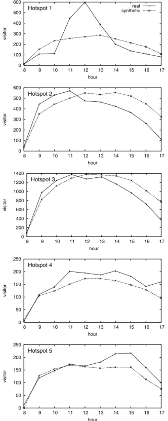
Figures 21 shows the number of visitors per region per hour. Thex-axis shows one-hour buckets starting at 08:00 and end-ing at 18:00. The number of visitors usend-ing the synthetic tracks are similar to the real tracks for all regions except hotspot 1. The number of visitors in the real tracks for these four hotspots is relatively stable during the day. Visitors increase at the beginning of the day, are relatively constant during the day, and decrease at the end of the workday. Hotspot 1, however, has a large peak between 1200 and 1300, which may be due to users visiting a restaurant during their lunch hour. The synthetic tracks of hotspot 1 fail to match the real behavior due to these temporal variations. While our model considers the variations for the beginning and ending of each working day, it currently does not consider the variation for certain hours during the day, such as lunch time. Incorporating such temporal variations may be useful, although it may require prior knowledge about a hotspot, such as whether it contains a restaurant, if lunch-time movements are to be considered.

We compute the relative error for each hotspot. Let the value of a real track berand that of synthetic track bes. Then, the relative error is defined as n_i=1|ri−si|/n_i=1ri where n

is the number of hour-long bins.

Figure 22 shows the relative error between the synthetic tracks and real tracks. Hotspot 1 with a large peak during lunch time has the largest error of 46%. The error for the rest of the hotspots ranges from 16% to 30%. The median of relative error for the five regions is 17%.

VII. RELATED WORK

Most MANET researchers use relatively simple mobility models, based on some form of random walk on a flat plane. With increasing awareness of the limitations of some of these models [16] and the importance of a realistic mobility model in the evaluation of MANET protocols [17], others have begun to propose more complex models. For example, Jardosh et al. propose a random-walk model that incorporates obstacles [18]. This paper describes a technique for modeling

0 100 200 300 400 500 600 8 9 10 11 12 13 14 15 16 17 visitor hour

Hotspot 1 _syntheticreal

0 100 200 300 400 500 600 8 9 10 11 12 13 14 15 16 17 visitor hour Hotspot 2 0 200 400 600 800 1000 1200 1400 8 9 10 11 12 13 14 15 16 17 visitor hour Hotspot 3 0 50 100 150 200 250 8 9 10 11 12 13 14 15 16 17 visitor hour Hotspot 4 0 50 100 150 200 250 8 9 10 11 12 13 14 15 16 17 visitor hour Hotspot 5

Fig. 21. Hourly visitors.This figure shows the number of visitors during each hour of a workday for the five hotspots.

paths between points based on Voronoi diagrams, which could be adapted for use in our model. Another mobility model is proposed by Musolesi et al. [19], who use observations from social networking theory to create a model that reflects how users congregate according to their social relationships

1 2 3 4 5 0 0.1 0.2 0.3 0.4 0.5 Hotspot Relative error

Fig. 22. Relative error.This figure shows the relative error between the synthetic tracks and the real tracks.

with each other. These complex models, however, are typically synthetically generated, rather than based on real traces.

Recently, there have been a few papers describing ways to extract places from traces of user mobility. For exam-ple, Patterson et al. used GPS data in an effort to identify common destinations in a user’s daily life [20]; their results are interesting, but it is not clear how to use this technique to derive a general model for a user population. Similarly, Kang et al. demonstrate a method for clustering a sequence of location observations to identify “places” within a moving user’s path [21]. Again, although they validate the technique on a trace of two users, their aim is not to build a general model for a larger population.

There have been few significant efforts to create mobility models from real traces. In one short paper, Hsu et al. develop a Weighted Way Point model from a set of survey data, in which they asked 268 students to keep a diary of their movements on campus for a month, at the granularity of a building [22]. Using a predefined set of five location types (classrooms, libraries, cafeterias, off-campus, and other), they noted a non-uniform distribution of visits to these location types. Their Markov-based model conditions the choice of a next location type upon the time of day (morning or afternoon) and on the current location type. They also used the survey data to extract a distribution of pause times for each location type. They confirm that their model, when used in a simulator for ad hoc routing, does demonstrate non-uniform location distribution and (due to clustering) leads to lower connectivity than does the random way-point model. Although our study must estimate user locations from network-association records, it goes far beyond their study, by extracting mobility for a larger area, with finer location granularity, over a longer period of time, and for far more users. Another study based on observations of pedestrian traffic on a campus [23] developed a hybrid mobility model which favors certain directions based on probabilities computed from the observations. In this short paper, they only observe people at six locations on a large campus. Using the same trace as our study, Jain et al. [24] developed a model of wireless users’ AP registration patterns, which may be significantly different from users’ physical mobility patterns. Their model ignores temporal patterns and focuses only on spatial patterns.

VIII. CONCLUSION

This paper has presented one of the first attempts to construct a WLAN mobility model from real-world wireless user traces. We present a method for extracting users’ mo-bility tracks from these traces, and validated this method by comparing them to the location determined by users carrying both GPS and 802.11 devices. We applied our method to one of the largest available traces of wireless users, from Dartmouth College. By examining the mobility in these tracks we were able to extract information about the movement speed, pause times, destination transition probabilities, and waypoints between destinations. This information forms an empirical model that we used to generate synthetic tracks, which we validated by comparison to the real tracks. We found that our generated tracks produced similar results to the real tracks, save in the cases where temporal variations were present in the real tracks, as our model does not consider these temporal effects.

We believe that this model, and the methods used to construct it, will be useful for research in many areas of mobile computing and communications. As examples, we cite related work in mobile ad hoc networking, opportunistic networking, content-distribution networks, and location prediction, all of which need good mobility models or an understanding of mobility characteristics.

In future work, we intend to further improve our metrics for validating our synthetic tracks. We also intend to help the research community use our model by developing a track generator capable of creating mobility traces that can be used by the network simulator ns-2.

ACKNOWLEDGMENTS. We would like to thank Udayan Deshpande, Tristan Henderson, and Libo Song for their help in collecting sample traces. Tristan also read earlier drafts of this paper and suggested improvements to the presentation. We also thank Stephen Paul for commenting on the Kalman filter. This project was supported by Cisco Systems, NSF Award EIA-9802068, and Dartmouth’s Center for Mobile Computing.

REFERENCES

[1] A. Roy, S. D. Bhaumik, A. Bhattacharya, K. Basu, D. J. Cook, and S. Das, “Location aware resource management in smart homes,” in

Proceedings of the First IEEE International Conference on Pervasive

Computing and Communications. Fort Worth, TX: IEEE Computer

Society Press, March 2003, pp. 481–488.

[2] L. Song, D. Kotz, R. Jain, and X. He, “Evaluating location predictors with extensive Wi-Fi mobility data,” inProceedings of the 23rd Annual Joint Conference of the IEEE Computer and Communications Societies

(INFOCOM), vol. 2, March 2004, pp. 1414–1424.

[3] J. Su, A. Chin, A. Popivanova, A. Goel, and E. de Lara, “User mobility for opportunistic ad-hoc networking,” inProceedings of the Sixth IEEE

Workshop on Mobile Computing Systems and Applications (WMCSA),

Lake District, England, Dec. 2004, pp. 41–50.

[4] A. Chaintreau, P. Hui, C. Diot, J. Scott, and J. Crowcroft, “Pocket switched networks: Real-world mobility and its consequences for op-portunistic forwarding,” University of Cambridge Computer Laboratory, Tech. Rep. UCAM-CL-TR-617, Feb. 2005.

[5] T. Henderson, D. Kotz, and I. Abyzov, “The changing usage of a mature campus-wide wireless network,” in Proceedings of the Tenth Annual International Conference on Mobile Computing and Networking

(MobiCom). ACM Press, September 2004, pp. 187–201.

[6] D. Kotz and K. Essien, “Analysis of a campus-wide wireless network,”

Wireless Networks, vol. 11, pp. 115–133, 2005.

[7] M. McNett and G. M. Voelker, “Access and mobility of wireless PDA users,” Department of Computer Science and Engineering, University of California, San Diego, Tech. Rep. CS2004-0780, February 2004. [8] J. I. Hong and J. A. Landay, “A architecture for privacy-sensitive

ubiquitous computing,” in Proceedings of the second international

conference on mobile systems, applications, and services (MobiSys),

Boston, MA, 2004, pp. 177–189.

[9] T. Buchholz and C. Linnhoff-Popien, “Towards realizing global scal-ability in context-aware systems,” in Proceedings of the International

Workshop on Location- and Conext-Awareness (LoCA).

Oberpfaffen-hofen, Germany: Springer-Verlag, May 2005, pp. 26–39.

[10] A. LaMarca, Y. Chawathe, S. Consolvo, J. Hightower, I. Smith, J. Scott, T. Sohn, J. Howard, J. Hughes, F. Potter, J. Tabert, P. Powledge, G. Borriello, and B. Schilit, “Place Lab: Device positioning using radio beacons in the wild,” inProceedings of Pervasive, Munich, Germany, 2005.

[11] Y.-C. Cheng, Y. Chawathe, A. LaMarca, and J. Krumm, “Accuracy char-acterization for metropolitan-scale Wi-Fi localization,” Intel Research Seattle, Tech. Rep. IRS-TR-05-003, Jan. 2005.

[12] H. Satoh, S. Ito, and N. Kawaguchi, “Position estimation of wire-less access point using directional antennas,” in Proceedings of the

International Workshop on Location- and Conext-Awareness (LoCA).

Oberpfaffenhofen, Germany: Springer-Verlag, May 2005, pp. 144–156. [13] L. Liao, D. Fox, and H. Kautz, “Learning and inferring transportation routines,” in Proceedings of the National Conference on Artificial

Intelligence, 2004, pp. 348–353.

[14] E. Welbourne, J. Lester, A. LaMarca, and G. Borriello, “Mobile context inference using low-cost sensors,” inProceedings of the International

Workshop on Location- and Conext-Awareness (LoCA).

Oberpfaffen-hofen, Germany: Springer-Verlag, May 2005, pp. 254–263.

[15] A. M. Law and W. D. Kelton,Simulation modeling and analysis, 3rd ed. McCraw-Hill, 2000.

[16] J. Yoon, M. Liu, and B. Noble, “Sound mobility models,” inProceedings of the Ninth Annual International Conference on Mobile Computing and

Networking. ACM Press, 2003, pp. 205–216.

[17] T. Camp, J. Boleng, and V. Davies, “A survey of mobility models for ad hoc network research,”Wireless Communications & Mobile Computing (WCMC): Special issue on Mobile Ad Hoc Networking: Research,

Trends and Applications, vol. 2, no. 5, pp. 483–502, 2002.

[18] A. Jardosh, E. M. Belding-Royer, K. C. Almeroth, and S. Suri, “Towards realistic mobility models for mobile ad hoc networks,” inProceedings of the Ninth Annual International Conference on Mobile Computing and

Networking. ACM Press, 2003, pp. 217–229.

[19] M. Musolesi, S. Hailes, and C. Mascolo, “An ad hoc mobility model founded on social network theory,” in Proceedings of the 7th ACM International Symposium on Modeling, analysis and Simulation of

Wireless and Mobile systems (MSWiM). Venice, Italy: ACM Press,

Oct. 2004, pp. 20–24.

[20] D. J. Patterson, L. Liao, K. Gajos, M. Collier, N. Livic, K. Olson, S. Wang, D. Fox, and H. Kautz, “Opportunity Knocks: a System to Pro-vide Cognitive Assistance with Transportation Services,” inProceedings

of UbiComp 2004: International Conference on Ubiquitous Computing,

ser. Lecture Notes in Computer Science, vol. 3205. Springer-Verlag, October 2004, pp. 433–450.

[21] J. H. Kang, W. Welbourne, B. Stewart, and G. Borriello, “Extracting places from traces of locations,” in Proceedings of the 2nd ACM International Workshop on Wireless Mobile Applications and Services

on WLAN Hotspots (WMASH), Philadelphia, PA, USA, 2004, pp. 110–

118.

[22] W. Hsu, K. Merchant, H. Shu, C. Hsu, and A. Helmy, “Weighted waypoint mobility model and its impact on ad hoc networks - MobiCom 2004 poster abstract,”Mobile Computing and Communications Review, Jan. 2005.

[23] D. Bhattacharjee, A. Rao, C. Shah, M. Shah, and A. Helmy, “Empirical modeling of campus-wide pedestrian mobility: Observations on the USC campus,” inProceedings of the IEEE Vehicular Technology Conference, September 2004.

[24] R. Jain, D. Lelescu, and M. Balakrishnan, “Model T: an empirical model for user registration patterns in a campus wireless LAN,” inProceedings of the Eleventh Annual International Conference on Mobile Computing

and Networking (MobiCom), Cologne, Germany, Aug. 2005, pp. 170–