Recursive Timed Automata
Ashutosh Trivedi and Dominik Wojtczak Computing Laboratory, Oxford University, UK
Abstract. We study recursive timed automata that extend timed automata with recursion. Timed automata, as introduced by Alur and Dill, are finite automata accompanied by a finite set of real-valued variables called clocks. Recursive timed automata are finite collections of timed automata extended with special states that correspond to (potentially recursive) invocations of other timed automata from their collection. During an invocation of a timed automaton, our model permits passing the values of clocks using both pass-by-valueandpass-by-referencemechanisms. We study the natural reachability and termination (reachability with empty invocation stack) problems for recursive timed automata. We show that these problems are decidable (in many cases with the same complexity as the reachability problem on timed automata) for recursive timed automata satisfying the following condition: during each invocation either all clocks are passed by reference or none is passed by reference. Furthermore, we show that for recursive timed automata that violate this condition reachability/termination problems are undecidable for automata with as few as three clocks. We also establish similar results for two-player game extension of our model against reachability/termination objective.
1
Introduction
Recursion is one of the central ideas in mathematics and computer science. Informally, recursion is a process in which objects are defined in terms of other objects of same type. For instance, recursive state machines[1] are defined as collection of rather peculiar state machines whose states, in addition to being states in usual sense, are allowed to be other state machines, including themselves; or in other words, some states may correspond to potentially recursive invocation of other state machines. Similarly,recursive Markov decision processes[14] are collection of special Markov decision processes whose states may correspond to the invocation of other Markov decision processes. Following this line of work, we define recursive extension of timed automata [2] and study reachability and termination problems for this model.
Timed automata are finite automata—a finite set of locations and a finite set of transitions—coupled with a finite set of continuous variables, called clocks, which grow with uniform slope. Simple form of constraints on clocks are allowed to appear as guards on the transitions and as location invariants. Syntax of timed automata also permits resetting the clocks to zero. The reachability problem for timed automata with at least three clocks is known to be PSPACE-complete, while the reachability problem is NLOGSPACE-complete for timed automata with one clock.
Recursive timed automaton consists of finite number ofcomponents where each component is a special form of timed automaton with specially marked entry and exit
locations. Moreover components can also have special form of locations, calledboxes, that correspond to recursive invocation of other components. We allow passing the values of clocks to the invoked component in the sense that the values of these clocks are available to the invoked component, and passed clocks grow normally while the invoked component is under execution. Moreover, the passed clocks can be used in guards and location invariants inside the component, and transitions of the component may reset these clocks to zero. We allow two different mechanisms of passing the clocks: 1) pass-by-value, where upon returning from the invoked component clocks assume the value prior to the invocation; and 2)pass-by-reference, where upon returning from the invoked component their value is unaltered (it is as if a copy of these clocks is restored in the calling component). We say that a clock isglobalif it is always passed by reference, and it islocalif it is always passed by value. Notice that, since there is no bound on the depth of recursive calls in our model, we will need to be able to analyse potentially infinitely many clocks, but at any point of the execution only a fixed number of them is not stopped.
We study reachability and termination (reachability of one of the exits with the empty calling context) problems on recursive timed automata. We show that the reachability problem of recursive timed automata is decidable, and EXPTIME-complete, if for every component, either all clocks of that component are passed by reference or none is passed by reference. Moreover, we study reachability games on recursive time automata, where the control state determines which of the two players picks the action to be performed. The objective of one player is reaching a particular subset of the control states, while the objective of the other player is complementary, i.e. avoiding them forever throughout the run of the recursive time automaton. We show that determining the winner of such games is in 2EXPTIME.
Applications. Much in the same way as recursive state machines can modelBoolean programs [4] (or more general software systems using predicate abstraction [16]), it can be argued that recursive timed automata can model hard real-time software systems [8]. The need to use the dense semantics of time is more pressing in the case of real-time distributed software systems, i.e., computer programs that run on multiple autonomous computers communicating through computer network. Even after disallowing concurrency, verifying the correctness of real-time distributed software is a fantastic challenge as each participating computer has its own physical clock of varying frequency, while no global clock is available. Under such circumstances it is impossible to model system using discrete semantics of time without knowing the clock frequencies of participating computers. Hence it is natural to study these systems with dense semantics of time.
In [9], the authors study the problem of automatic generation of an optimal controller for an oil pump by defining this model as a 2-player game played on a time automaton. The actual controller used in practice for controlling this oil pump was a 400 lines long C program. Most C programs, apart from the simplest ones, make use of functions and recursive invocations of one function by another. Parameters to such functions are either passed by value or by reference (which in C language is done explicitly by passing a pointer). These kind of controllers operate on variables that are constantly growing in real-time, e.g. total time, oil pressure, temperature etc. The
natural model to study correctness of such a system is a game played on recursive timed automaton with a safety critical objective, i.e. the aim for the controller is to avoid a certain set of bad states, while the aim of the other player, the “malicious environment”, is trying to reach one of these states. If the controller has a winning strategy, i.e. no matter what how the environment behaves, none of the unsafe states will ever be reached, then the implementation of the controller is correct.
Related work. All the work with pushdown timed automata, see e.g. [10,11], has considered only global clocks. Bouajjani, Echahed, and Robbana [5] studied linear hybrid automata with pushdown stack and counters, and showed decidability of reachability in pushdown timed systems. Emmi and Majumdar [13] showed the decidability of language inclusion for implementation as timed pushdown automata and specification as timed automata with one clock; however they proved that it is undecidable when the specification is visibly pushdown timed automata even with one clock [13]. The work on timed automata with counters [7] studies extending time automata with multiple counters. The reachability problem for such systems is already undecidable without clocks, so the authors study several decidable subclasses of this model. Context-Free Timed Systems, studied in [6], are less expressive than our model, and [6] shows decidability of various verification problems for context-free timed systems with linear-hybrid observers (a variable that cannot be used in the constraints used on any edge, similar to prices/cost variables in timed automata).
The paper is organised as follows. In the next section we set definitions of key concepts like labelled transition systems, games, and recursive state machines. In Section 3 we introduce our model and define problems studied in this paper. In Section 4 we prove the undecidability of termination problem and games on the general model, while in Section 5 we discuss decidable subclasses and give complexity results.
2
Definitions
2.1 Preliminaries
Notation. We assume, the sets N of non-negative integers, R of reals and R⊕ of
non-negative reals. Forn ∈ N, letJnKNandJnKR denote the sets{0,1, . . . , n}, and
{r∈R|0≤r≤n}respectively.
Labelled Transition System. A labelled transition system (LTS) is a tuple L = (S, A, X)whereS is the set ofstates,Ais the set ofactions, andX : S ×A → S
is thetransition function. We say that an LTSLisfinite(discrete) if bothS andAare finite (countable). We writeA(s)for the set of actions available ats∈S, i.e., the set of actionsa∈Afor whichX(s, a)is non-empty.
We say that(s, a, s0) ∈ S ×A×S is a transition of L if s0 = X(s, a)and a
runof Lis a sequencehs0, a1, s1, . . .i ∈ S×(A×S)∗ such that(si, ai+1, si+1)is a
transition ofLfor alli ≥0. We writeRunsL(FRunsL) for the sets of infinite (finite) runs andRunsL(s)(FRunsL(s)) for the sets of infinite (finite) runs starting from states. For a finite runr=hs0, a1, . . . , sniwe writelast(r)=sn for the last state of the run. A strategy inL is a functionσ : FRunsL → Asuch that for all runsr ∈ FRunswe have that σ(r) ∈ A(last(r)). We write ΣL for the set of strategies in L. For a state
s∈Sand a strategyσ∈ΣL, we write Run(s, σ)for the unique runhs0, a1, s1, . . .i ∈
RunsL(s)such thats0 = sand for every i ≥ 0we have that σ(rn) = an+1, where rn=hs0, a1, . . . , sni(herer0=hs0i). For a setF ⊆Sand a runr=hs0, a1, . . .iwe
defineStop(F)(r) = inf{i∈N : si ∈F}.
Given a states ∈ S and a set of final statesF ⊆ S we say that a final state is reachable froms0if there is a strategyσ∈ΣLsuch thatStop(F)(Run(s, σ))<∞. A
reachability problemis to decide whether in a given LTS a final state is reachable from a given initial state.
Games on Labelled Transition Systems. Agame arenaGis a tuple(L, SAch, STor), whereL = (S, A, X)is an LTS,SAch ⊆ S is the set of states controlled by player Achilles, andSTor⊆Sis the set of states controlled by player Tortoise. Moreover, sets
SAchandSTorform a partition of the setS.
A strategy of player Achilles is a partial functionα:FRunsL →Asuch that for a runr∈FRunsLwe have thatα(r)is defined iflast(r)∈SAch, andα(r)∈A(last(r)) for every suchr. A strategy of player Tortoise is defined analogously. LetΣAchL and
ΣTorL be the set of strategies of player Achilles and Tortoise, respectively. The unique run Run(s, α, τ)from a stateswhen players use strategiesα∈ΣL
Ach andτ ∈ΣLToris defined in a straightforward manner.
In areachability gameon G, rational players Achilles and Tortoise take turns to move a token along the states ofL. The decision to choose the successor state is made by the player controlling the current state. The objective of Achilles is to eventually reach certain states, while the objective of Tortoise is to avoid them forever. For an initial state sand a set of final statesF, the lower value ValLF(s)of the reachability game is defined as the upper bound on the number of transitions that Tortoise can ensure before the game visits a state in F irrespective of the strategy of Achilles, and is equal tosupτ∈ΣL
Torinfα∈ΣAchL Stop(F)(Run(s, α, τ)). The concept of upper value is ValLF(s)is analogous and defined asinfα∈ΣL
Achsupτ∈Σ L
TorStop(F)(Run(s, α, τ)). If ValLF(s) =Val
L
F(s)then we say that the reachability game is determined, or the value ValLF(s)of the reachability game exists and it is such that ValLF(s) =ValLF(s) =Val
L
F(s). We say that Achilles wins the reachability game if ValLF(s)<∞. Areachability game problemis to decide whether in a given game arenaG, an initial statesand a set of final statesF, player Achilles has a strategy to win the reachability game.
2.2 Recursive State Machines
Recursive state machines (RSMs) generalise LTSs, and can be used to model systems exhibiting recursion and non-deterministic behaviour.
Definition 1 ([1]).Arecursive state machineM= (M1,M2, . . . ,Mk)is a tuple of components, where for each1≤i≤kcomponentMi= (Ni, Eni, Exi, Bi, Yi, Ai, Xi) consists of:
– a finite setNiof nodes, including the setEniofentry nodesand the (disjoint from
Eni) setExiofexit nodes.
M1 u1 u2 u4 b1:M2 b2:M3 u3 M2 v1 v2 v3 v4 c1:M2 c2:M3 M3 w1 w2 d:M1
Fig. 1.Example recursive state machine taken from [1]
– boxes-to-components mappingYi:Bi→ {1,2, . . . , k}that assigns every box to a component. To each boxb∈Biwe associate a set of call portsCall(b), and a set of return portsRet(b):
Call(b) =
(b, en) : en∈EnYi(b) , andRet(b) =
(b, ex) : ex∈ExYi(b) . LetCalli=∪b∈BiCall(b)andReti=∪b∈BiRet(b)be the set of call and return ports of componentMi. We writeQi = Ni∪Calli∪Reti for the union of the set of nodes, call ports and return ports, and we collectively refer to them as the verticesof the componentMi.
– a finite setAiofactions.
– atransition functionXi : Qi×Ai →Qi with a condition that call ports and exit nodes do not have any outgoing transitions.
For the sake of simplicity, we assume that the set of boxes B1, . . . , Bk and set of nodesN1, N2, . . . , Nk are mutually disjoint. We use symbols N, B, A, Q, X, etc. to denote the union of the corresponding symbols over all components. For example,
N =∪k i=1Ni.
Example 2. The visual presentation of a finite recursive state machine with three components M1, M2, and M3 is depicted in Figure 1. Components are shown as
thinly framed rectangles with their labels written close to upper right corner, e.g. see componentM1. Nodes of the components are shown as circles with their labels written
inside them, e.g. see nodeu1. Entry nodes of a component appear on the left of the
component (seeu1), while exit nodes appear on the right (seeu4). Boxes are shown
as thickly framed rectangles inside components labelled b : M, where bis the label of the box andM is the component it is mapped to. Call ports of boxes are drawn as small circles on the left of the box, while return ports are on the right. We omit labelling the call and return ports as these labels are clear from their position on the boxes. For example, call port(b1, v1)is the top small circle on the left-hand side of boxb1, since
boxb1is mapped toM2andv1is the top node on its left-hand side.
Intuitively, a run of an RSM starts at one of the entries of its components and proceeds via the edges from one state to another until it reaches an entry port of a box or an exit of the current component. In the former, this box is pushed onto thestack of pending (recursive) callsand the run starts from the corresponding entry of the component this box is mapped to. In the latter, if the stack of pending calls is empty then the run terminates; otherwise, it pops the box from the top of the stack and jumps to the exit port (of the just popped box) corresponding to the just reached exit of the component.
Formally, the semantics of a recursive state machine is given by a discrete LTS, whose states are pairs consisting of a sequence of boxes, called the context, and a vertex.
The context corresponds to the sequence of unreturned component calls, and the vertex is a vertex of the current component.
Definition 3 (RSM semantics).LetM= (M1,M2, . . . ,Mk)be an RSM where the componentMiis(Ni, Eni, Exi, Bi, Yi, Ai, Xi). The semantics ofMis the countable labelled transition system[[M]] = (SM, AM, XM)where:
– SM⊆B∗×Qis the set of states; – AM=∪ki=1Aiis the set of actions;
– XM:SM×AM→SMis the transition function such that fors= (hκi, q)∈SM
anda∈AM, we have thats0 =XM(s, a)if and only if one of the following holds:
1. the vertexqis a call port, i.e.q= (b, en)∈Call, ands0= (hκ, bi, en); 2. the vertexqis an exit node, i.e.q=ex ∈Exands0 = (hκ0i,(b, ex))where
(b, ex)∈Ret(b)andκ= (κ0, b);
3. the vertexqis any other kind of vertex, ands0= (hκi, q0)andq0∈X(q, a). A given M and a subsetQ0 ⊆ Q of its nodes we define the set [[Q0]]M as the set
{(hκi, v0) : κ∈B∗andv0∈Q0}. We also define the set of terminal configurations TermMas the set{(hεi, ex) : ex∈Ex}.
Given a recursive state machineM, an initial nodev, and a set of final vertices
F ⊆Qthereachability problemonMis defined as the reachability problem on the LTS[[M]]with the initial state (hεi, v)and the set of final states[[F]]. We also define termination problemas the reachability problem of one of the exits with the empty context. Hence, given a recursive state machineMand an initial nodev, the termination problem onMis defined as the reachability problem on LTS[[M]]with the initial state (hεi, v)and the set of final statesTermM. It is easy to show that the reachability problem
is at least as hard as the termination problem. We can see this on the example in Figure 1: if we can decide whether stateu3is reachable from(hεi, u2), we will also know whether
it is possible to terminate from(hεi, w1)(simply because it is impossible to reach node u3from(hεi, w1)). Hence, all the complexity upper bounds for the reachability problem
in this paper apply also to the termination problem, and all the complexity lower bounds for the termination problem apply also to the reachability problem.
Games on Recursive State Machines. A partition (QAch, QTor) of vertices Q of an RSMM(between players Achilles and Tortoise) gives rise to recursive game arena
G = (M, QAch, QTor). Given an initial state, v, and a set of final states, F, the reachability game on M is defined as the reachability game on the game arena ([[M]],[[QAch]]M,[[QTor]]M) with the initial state (hεi, v) and the set of final states
[[F]]M. Also, the termination game M is defined as the reachability game on the
game arena([[M]],[[QAch]]M,[[QTor]]M)with the initial state(hεi, v)and the set of final
statesTermM. It is a well known result (see, e.g. [22,15]) that reachability games and
termination games on RSMs are determined.
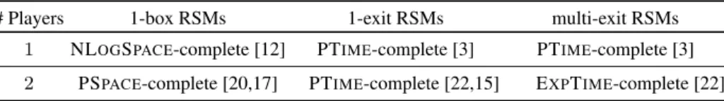
Complexity results for RSMs and their subclasses. The two most natural subclasses of RSMs are1-box RSMsand1-exit RSMs. 1-box RSMs are these RSMs that have just a single component and a single box inside of it (this box of course has to be mapped to that single component). On the other hand, an RSM is a 1-exit RSM iff each of its components has just one exit (and hence also all of its boxes), i.e.Exiis a singleton for
# Players 1-box RSMs 1-exit RSMs multi-exit RSMs
1 NLOGSPACE-complete [12] PTIME-complete [3] PTIME-complete [3]
2 PSPACE-complete [20,17] PTIME-complete [22,15] EXPTIME-complete [22]
Table 1.Complexity results for reachability objective for RSMs
all possiblei-s. The general class of RSMs is sometimes referred to asmulti-exit RSMs. Table 1 summarises some key results for RSMs and their subclasses.
The results for 1-box RSMs are derived from the corresponding results for one-counter automata (for their definition, see, e.g. [18]), due to their exact correspondence: the counter value is equal to the number of boxes in the calling context, calling a box results in increasing the counter by1, while reaching an exit corresponds to decreasing the counter by1.
3
Recursive Timed Automata
Recursive timed automata (RTAs) extend classical timed automata [2] (TAs) with recursion feature similar to RSMs. Instead of defining TAs explicitly, we directly define RTAs whose degenerate case corresponds to TAs. Just as a TA is a finite automaton with a finite set of clocks (continuous variables), a recursive timed automaton is an RSM with a finite set of clocks which can be passed to components during invocation either by value or by reference. Before formally defining the syntax and semantics of RTA we need to introduce the concept of clock valuations, regions and zones.
3.1 Clocks, clock valuations, regions and zones.
LetCbe a finite set ofclocks. In the definition of recursive timed automata (and timed automata [2]) constraints on clocks may appear in the guards on the transitions, where a clock or the difference of two clocks can be compared against natural numbers (in general with rational numbers). LetKbe the largest such number. The set ofclock constraintsoverCis the set of conjunctions ofsimple constraints, which are constraints of the formc ./ iorc−c0 ./ i, wherec, c0 ∈ C,i∈JKKN, and./ ∈ {<, >,=,≤,≥}. Let SCC be the finite set of simple clock constraints.
Aclock valuation on C is a function ν : C → R⊕ and we writeV for the set
of clock valuations. For a clock valuation ν ∈ V and delay t ∈ R⊕ we write ν+t
for the clock valuation defined by (ν+t)(c) = ν(c)+t, for all c ∈ C. For a subset of clocks C ⊆ C and a clock valuation ν0 ∈ V, we writeν[C:=ν0] for the clock valuation whereν[C:=ν0](c) = ν0(c)ifc ∈ C, and ν[C:=ν0](c) = ν(c)otherwise. Clock valuation0∈V is a special valuation such that0(c) = 0for allc∈ C. Hence, forC ⊆ C, we writeν[C:=0]for the clock valuation whereν[C:=0](c) = 0ifc∈C, andν[C:=0](c) =ν(c)otherwise.
A clock region is a maximal set ζ ⊆ V, such that SCC(ν)=SCC(ν0) for all ν, ν0∈ζ. We write R for the finite set of clock regions. Every clock region is an equivalence class of the indistinguishability-by-clock-constraints relation, and vice versa. Note thatν andν0 are in the same clock region if and only if the integer parts of the clocks and the partial orders of the clocks, determined by their fractional parts, are the same in ν andν0. We write[ν]for the clock region of ν. For a clock region
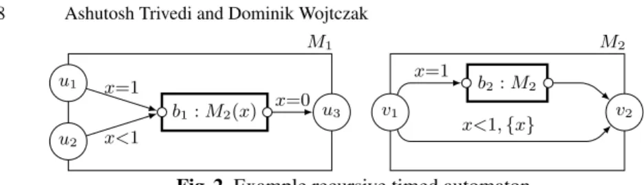
M1 u1 u2 u3 b1:M2(x) x=1 x<1 x=0 M2 v1 v2 b2:M2 x=1 x<1,{x}
Fig. 2.Example recursive timed automaton
{[ν0[C:=ν]] : ν0∈ζ}. Observe that ifν =0then the setζ[C:=0]is a singleton, and we sometimes abuse the notation to writeζ[C:=0]for the unique region.
Aclock zoneis a convex set of clock valuations, which is a union of a set of clock regions. We writeZfor the set of clock zones. A set of clock valuations is a clock zone if and only if it is definable by a clock constraint.
3.2 Syntax
Definition 4 (Syntax). A recursive timed automaton T = (C,(T1,T2, . . . ,Tk))is a pair made of a set of clocksCand a collection of components(T1,T2, . . . ,Tk). Each componentTi= (Ni, Eni, Exi, Bi, Yi, Ai, Xi, Pi,Invi, Ei, ρi)consists of:
– a finite setNiofnodes, including the setEniof entry nodes and the (disjoint from
Eni) setExiof exit nodes;
– a finite setBiofboxes;
– boxes-to-components mappingYi:Bi→ {1,2, . . . , k}that assigns every box to a component; (Call portsCall(b)and return portsRet(b)of a boxb∈Bi, and call portsCalliand return portsRetiof a componentTiare defined as before. We set
Qi=Ni∪Calli∪Retiand refer to this set as the set of vertices ofTi.)
– a finite setAiofactions;
– thetransition functionXi :Qi×Ai →Qiis with the condition that call ports and exit nodes do not have any outgoing transitions;
– pass-by-value mappingPi :Bi →2C that assigns every box the set of clocks that are passed by value to the component mapped to the box; (The rest of the clocks are assumed to be passed by reference.)
– theinvariant conditionInvi:Qi→ Z;
– theaction enabledness functionEi:Qi×Ai → Z; and
– theclock reset functionρi:Ai→2C.
We assume that the sets of boxes, nodes, etc. are mutually disjoint and we use symbols (N, B, Y, Q, P, X, etc.) without a subscript, to denote the union of the corresponding objects over all components. When we consider an RTA as an input of an algorithm, its size should be understood as the sum of the sizes of encodings ofQ,C,Inv,A,E, andX. Analogously as for RSMs, we define special subclasses of RTAs:1-exit RTAs, for which each component is allowed to have just one exit, and1-box RTAs, that just consist of a single component with a single box inside of them.
We say that a recursive timed automaton isglitch-free if for every box either all clocks are passed by value or none is passed by value, i.e. for eachb∈Bwe have that eitherP(b) =CorP(b) =∅. Any general recursive timed automaton with one clock is trivially glitch-free.
Example 5. The visual presentation of a recursive timed automaton with two compo-nentsM1andM2, and one clockxis shown in Figure 2. The visual representation is
similar to that in RSMs. However, each transition is labelled with a guard and the clocks to be reset, (e.g. transition from nodev1tov2can be taken only when clockx<1, and
after taking this transition, clockxis reset), and a box is labelled asb:M(C)to denote that boxbis mapped toM and all the clocks in the setCare passed by value, and the rest of the clocks are passed by reference. When the setCis empty, we just writeb:M
forb:M(∅).
3.3 Semantics
Aconfigurationof an RTAT is a tuple(hκi, q, ν), whereκ∈(B×V)∗is (possibly empty) sequence of pairs of boxes and clock valuations,q∈Qis a vertex andν∈V is a clock valuation overCsuch thatν∈Inv(q). The sequencehκi ∈(B×V)∗denotes the stack of pending recursive calls and the valuation of all the clocks at the moment that call was made, and we refer to this sequence as the context of the configuration. Technically, it suffices to store the valuation of clocks passed by value, because other clocks retain their value after returning from a call to a box, but storing all of them simplifies the notation. We denote the the empty context by hi. For any t ∈ R, we let(hκi, q, ν)+tequal the configuration(hκi, q, ν+t). Informally, the behaviour of an RTA is as follows. In configuration(hκi, q, ν)time passes before an available action is triggered, after which a discrete transition occurs. Time passage is available only if the invariant conditionInv(q)is satisfied while time elapses, and an actionacan be chosen after timetelapses only if it is enabled after time elapse, i.e., ifν+t∈E(q, a). If the actionais chosen then the successor state is(hκi, q0, ν0)whereq0 ∈δ(q, a)and
ν0 = (ν+t)[ρ(a) :=0]. Formally, the semantics of an RTA is given by an LTS which has both an uncountably infinite number of states and transitions.
Definition 6 (RTA semantics).LetT = (C,(T1,T2, . . . ,Tk))be an RTA where each component is of the form Ti = (Ni, Eni, Exi, Bi, Yi, Ai, Xi, Pi,Invi, Ei, ρi). The semantics ofT is a labelled transition system[[T]] = (ST, AT, XT)where:
– ST ⊆ (B×V)∗×Q × V, the set of states, is such that (hκi, q, ν) ∈ ST if ν∈Inv(q).
– AT =R⊕×Ais the set of timed actions;
– XT : ST ×AT → ST is the transition function such that for(hκi, q, ν) ∈ ST
and(t, a)∈AT, we have(hκ0i, q0, ν0) =XT((hκi, q, ν),(t, a))if and only if the
following condition holds:
1. if the vertexqis a call port, i.e.q = (b, en) ∈ Callthent = 0, the context hκ0i=hκ,(b, ν)i,q0=en, andν0=ν.
2. if the vertex q is an exit node, i.e. q = ex ∈ Ex, hκi = hκ00,(b, ν00)i, and let (b, ex) ∈ Ret(b), then t = 0; hκ0i = hκ00i; q0 = (b, ex); and
ν0 =ν[P(b):=ν00].
3. if vertexqis any other kind of vertex, thenν+t0 ∈Inv(q)for allt0 ∈ [0, t];
3.4 Reachability (Termination) Problems and Games
For a subset Q0 ⊆ Q of states of recursive timed automaton T we define the set[[Q0]]T as the set{(hκi, q, ν)∈ST : q∈Q0}. We also define the set of terminal
configurationTermT as the setTermT ={(hεi, q, ν)∈ST : q∈Ex}.
Given a recursive timed automatonT, an initial nodeqand valuationν ∈V, and a set offinal verticesF ⊆Q, thereachability problemonT is defined as the reachability problem on LTS[[T]]with the initial state(hεi, q, ν)and the set of final states[[F]]T. As
with RSMs, we also definetermination problemas reachability of one of the exits with the empty context. Hence, given an RTAT and an initial nodeqand a valuationν∈V, the termination problem onT is defined as the reachability problem on LTS[[T]]with the initial state(hεi, q, ν)and the set of final statesTermT.
Example 7. Consider the RTA shown in Figure 2. From the vertexu1ofM1there is no
path that visits the exit nodeu3with the empty calling context, as the only transition
available formu1is to wait until clockx= 1, and then invoking componentM2which
recursively calls itself forever if the value of clock x = 1. On the other hand, from nodeu2there are infinitely many paths that reachu3 with the empty context. Notice
that termination atu3is possible only when delay atu2is0time-units, as upon exiting
boxbclockxis tested against0. Since clockxwas passed by value to componentM2,
the current value of clockxis the one before the invocation ofM2, and hence the clock
reset insideM2does not help.
A partition(QAch, QTor)of verticesQof an RTAT gives rise to a recursive timed game arenaΓ = (T, QAch, QTor). Given an initial vertexq, a valuationν ∈ V and a set of final statesF, the reachability game onΓ is defined as the reachability game on the game arena([[T]],[[QAch]]T,[[QTor]]T)with the initial state(hεi,(q, ν))and the set of
final states[[F]]T. Also, termination game onT is defined as the reachability game on
the game arena([[T]],[[QAch]]T,[[QTor]]T)with the initial state(hεi,(q, ν))and the set of
final statesTermT.
4
Undecidability Results
The following is one of the key results of this paper.
Theorem 8. Termination problem is undecidable for recursive timed automata with at least three clocks. Moreover, termination game problem is undecidable for recursive timed automata with at least two clocks.
For the undecidability proofs we use reduction from the halting problem of two-counter Minsky machines [19]. A Minsky machine A is a tuple (L, C, D) where:
L={`0, `1, . . . , `n}is the set of states including the distinguished terminal state`n;
C={c1, c2}is the set of twocounters;D={δ0, δ1, . . . , δn−1}is the set of transitions
of the following type:
1. (incrementc)δi:c:=c+ 1; goto`k,
2. (test-and-decrementc)δi: if(c >0)then(c:=c−1;goto`k)else goto`m, wherec∈C,δi∈Dand`k, `m∈L.
A configuration of a Minsky machine is a tuple(`, c, d)where` ∈Landc, dare natural numbers that specify the value of countersc1 andc2, respectively. The initial
configuration is(`0,0,0). A run of Minsky machine is a (finite or infinite) sequence
of configurations hs0, s1, . . .i wheres0 is the initial configuration, and the relation
between subsequent configurations is governed by transitions at their respective states. The run is a finite sequence if and only if the last configuration is the terminal state`n. Note that a Minsky machine has only one run starting from the initial configuration. Termination problemfor a Minsky machine asks whether its unique run is finite. It is well known ([19]) that the termination problem for a two-counter Minsky machine is undecidable. In the rest of the section we show a reduction from the halting problem of Minsky machines to the termination games on RTA with two clocks. The reduction to the termination problem for (1-player) RTAs with three clocks is in the technical report version of this paper [21].
We fix the clocks set C = {x, y}, and we describe the construction of the central componentHALTA with nodes`0, `1, . . . , `n with the entry node`0 and the
exit node `n. A configuration (`i, c, d) of a Minsky machine corresponds to the configuration(hεi, `i, ν)such that ν(x) = 2−c ·3−d andν(y) = 0. Decrementing and incrementing counterc is simulated by doubling and halving, resp., of the clock
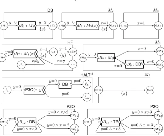
x, while decrementing and incrementing the counterd is simulated by tripling, and thirding1, resp., the value of clock x. Testing counter c (resp. d) against 0 can be simulated by multiplying clock xby some power of3 (resp.,2) and then comparing it against3 (resp.2). The components for doubling (DB) and halving (HF) the value of clockx, and testing whether the value of clockxis of the form2−ior3−i(P2Oor
P3O, resp.) are given in Figure 3. Due to space constraints, we omit the description of components for tripling,TR, and thirding,TH, of clockx. However such components are very similar to componentsDBandHF. All components function as intended only when upon entering them, the value of clockyis0. The vertices of these components are partitioned between Achilles and Tortoise: the only vertex controlled by Tortoise (shown as black squares) is the return port(B8, ex9)in componentM8. The component DB0, invoked from inside the component M8, is similar to gadget DB, however it
doubles the value of clocky, while assuming that clockxis set to0. We assume that the node labelled_¨ has no outgoing transitions. The behaviour of componentsP2O
andP3Ois as follows: if clockxis of the form2−iand3−i, resp., a run starting at that component’s entry will terminate at its bottom exit and if clock x is not of that form then such a run will terminate at that component’s top exit. Since the precise construction ofHALTAis straightforward, we just present in Figure 3 a schema that simulates the test-and-decrementcoperation:δi: if(c >0)then(c:=c−1;goto`k)else goto`m. Whenever a run reaches node`i insideHALTA, a box mapped toP3Ois called that tests whether the value of countercis zero. After returning fromP3Oboth clocks are restored and the exit port indicates whether clockcis zero or not. If clockcis zero then the run proceeds straight to node`m; otherwise the value of the countercis decremented by1by multiplying clockxby two using componentDBand the run proceeds to node
`k. It should be easy to see now how to encode the incrementcoperation and how to combine them all into theHALTAcomponent.
DB en1 B1:M2 ex1 y=0 y=2 {y} M2 en2 B2:M3(x) ex2 y=0 x=1 {x} M3 en3 x=1 ex3 HF en7 ¨ ^ ex7 B7:M8(x) u1 ¨ _ y=0 x=1 {x} y=1 {y} x=y x6=y en8 ex8 ex08 B8:M9 M8 B80 :DB0 y=0 x=0 x=0 x=0 M9 en9 ex9 {x} `i P3O(x, y) HALTA DB `k `m y=0 y=0 y=0 y=0 P2O en12 ex12 ex012 B12:DB y=0 y=0∧x>2 y=0∧x= 2 y=0∧x<2 P3O en13 ex13 ex013 B13:TR y=0 y=0∧x>3 y=0∧x= 3 y=0∧x<3
Fig. 3.Components for doublingDBand halvingHFthe value of clockx, and checking whetherxis of the form2−iand3−i.
To make the proofs more comprehensible, we show a run in an RTA using three different forms of transitions s −−→g,C t s0, s s0, ands
M(C)
−−−−→∗ s0 defined in the
following way.
1. The transitions of forms −−→g,C t s0, wheres = (hκi, n, ν), s0 = (hκi, n0, ν0)are configurations of an RTA,gis a clock constraint,Cis a set of clocks, andtis a real number, holds if there is a transition in the RTA from vertexnton0 with guardg
and clock reset setC, moreoverν0 = (ν+t)[C:=0].
2. The transitions of the form s s0, where s = (hκi, n, ν), s0 = (hκ0i, n0, ν0), correspond to the following cases:
(a) transitions from a call port to an entry node, i.e. ,n = (b, en)for some box
b∈Bandκ0 =hκ,(b, ν)iandn0 =en∈En, whileν0 =ν.
(b) transition from an exit node to a return port (which also restore the value of clocks passed by value), i.e.hκi = hκ00,(b, ν00)i,n = ex ∈ Ex, andn0 = (b, ex)∈Ret(b)andκ0=κ00, whileν0=ν[P(b) =ν00].
3. The transitions of the form s −M−−−(C→)∗ s0, called summary edges, where s =
(hκi, n, ν)), s0 = (hκ0i, n0, ν0) are such that n = (b, en)andn0 = (b, ex) are call and return ports, resp., of a boxbmapped toM which passes by value toM
For the sake of simplicity, in this section instead of presenting the context information in the form(b, ν)∈B×V, we write(b,(ν(x), ν(y)))if some clock is passed by value tob, else we just writeb. We also write a configuration(hκi, n, ν)as(hκi, n,(ν(x), ν(y))).
Proposition 9. For any contextκ∈(B×V)∗, any boxb∈B, andx
0∈[0,1]we have
that(hκi,(b, en1),(x0,0)) DB
−−→∗(hκi,(b, ex1),(2·x0,0)).
Proof. Component DB, shown in Figure 3, uses components M2 and M3. The
following is the unique run starting from the configuration (hκi,(b, en1),(x0,0))
terminating at the configuration(hκi,(b, ex1),(2·x0,0)).
(hκi,(b, en1),(x0,0)) (hκ, bi, en1,(x0,0)) y=0 −−→0 (hκ, bi,(B1, en2),(x0,0)) (hκ, b, B1i, en2,(x0,0)) y=0 −−→0 (hκ, b, B1i,(B2, en3),(x0,0)) (hκ, b, B1, B2(x0,0)i, en3,(x0,0)) x=1 −−→(1−x0) (hκ, b, B1, B2(x0,0)i, ex3,(1,1−x0)) (hκ, b, B1i,(B2, ex3),(x0,1−x0)) x=1,{x} −−−−−→(1−x0)(hκ, b, B1i, ex2,(0,2−2·x0)) (hκ, bi,(B1, ex2),(0,2−2·x0)) y=2,{y} −−−−−→(2·x0) (hκ, bi, ex1,(2·x0,0)).
The intermediate steps of this sequence of transitions can be easily verified. ut
Proposition 10. For any contextκ∈(B×V)∗, any boxb∈B, andx0∈[0,1], there
exists a unique strategy of Achilles such that either(hκi,(b, en7),(x0,0)) HF −−→∗(hκi,(b, ex7),( x0 2 ,0)), or(hκi,(b, en7),(x0,0)) HF −−→∗(hκi,(b,^¨),(x0, x0))).
Moreover, for other strategies of Achilles there exists a strategy of Tortoise such that componentHFdoes not terminate.
Proof. The main observation here is that, in componentHF, starting from the configu-ration(hκi,(b, en7),(x0,0))Achilles has a strategy to terminate only if he chooses to
delay the time by x0
2 in componentM9(called via boxB8). The evolution of the run
from (hκi,(b, en7),(x0,0))to(hκ, b, B7(x0,0), B8i, en9,(x0,0)) is straightforward.
Now, in componentM9Achilles can wait for an arbitrary amount of time before taking
a transition toex9and resetting clockx. Let us assume that he waits forttime units, and
hence(hκ, b, B7(x0,0)i,(B8, ex9),(0, t))is reached which is controlled by Tortoise.
Now Tortoise has a choice between making a transition toex8(believing thatt= x20)
or invoking the componentB80 (when suspecting thatt6=x0 2).
If Tortoise believes thatt = x0
2 then he makes a transition toex8 and thus the
system reaches the configuration(hκ, bi,(B7, ex8),(x0, t))giving rise to the following
run: (hκ, bi,(B7, ex8),(x0, t)) x=1,{x} −−−−−→(1−x0)(hκ, bi, u1,(0,1−x0+t)) y=1,{y} −−−−−→(x0−t)(hκ, bi, ex7,(x0−t,0)) (hκi,(b, ex7),(x0−t,0)).
Hence ift= x0
2 then the run terminates at configuration(hεi, ex7,(
x0 2,0)).
On the other hand if Tortoise believes thatt6= x0
2, then he invokes the component DB0to double the value of clocky(while keeping the value of clockxequal to0), and makes a transition, via exitex08, to the configuration(hκ, b, B7(x0,0)i, ex08,(0,2·t)).
Since x0 was passed by value, it is restored upon exiting from box B7 and the
configuration reached is(hκ, bi,(B7, ex80),(x0,2·t)). If Tortoise’s suspicion was right
and t 6= x0
2 then the only transition available to Achilles is to move to the _¨
vertex which never terminates. Otherwise Achilles can only move to configuration (hκi,(b,^¨),(x0, x0))and terminate. Hence, it is clear that the only winning strategy
for Achilles is to chooset=x0
2. ut
Proposition 11. For any contextκ∈(B×V)∗, any boxb∈B, andx0∈[0,1]we have
that starting from configuration(hκi,(b, en12),(x0,0))the componentP2Oterminates
at (hκi,(b, ex012),(x0,0)) only when x0 = 2−i for some i ∈ N and otherwise it
terminates at(hκi,(b, ex12),(x0,0)).
From Propositions 9, 10, and 11 (and similar results related to other components) it follows that Achilles has a strategy to terminate at`nin componentHALTAif and only if the Minsky machineAterminates.
5
Decidability Results
5.1 Region Abstraction
For every RTAT we define regional equivalence relationER ⊆ ST ×ST in the
following way: For configurations s = (hκi, q, ν) and s0 = (hκ0i, q0, ν0) we have that s, s0 ∈ ER, or equivalently we write [s] = [s0], if q = q0, [ν] = [ν0], and
κ= (b1, ν1),(b2, ν2), . . . ,(bn, νn) andκ0 = (b10, ν10),(b02, ν20), . . . ,(b0n, νn0)are such that for every1≤i≤nwe have[νi] = [νi0]andbi =b0i.
A relationB ⊆ST ×ST defined over the set of configurationsST of a recursive
timed automaton is a time-abstract bisimulation if for every pair of configurations
s1, s2 ∈ ST such that (s1, s2) ∈ B, for every timed action (t, a) ∈ AT such
that XT(s1,(t, a)) = s01, there exists a timed action (t0, a) ∈ AT such that XT(s2,(t0, a)) =s20 and(s01, s02)∈B.
Proposition 12. Regional equivalence relation for glitch-free recursive timed automata is a time-abstract bisimulation.
Proof. Let us fix configurationss= (hκi, q, ν)ands0 = (hκ0i, q0, ν0)such that[s] = [s0], timed action(t, a)∈XT such thatXT(s,(t, a)) =sa(= (κa,(qa, νa))). We need to find(t0, a)such thatX
T(s0,(t0, a)) = s0a(= (κ0a,(q0a, νa0)))and[sa] = [s0a]. There are following three cases.
1. The vertexqis a call port, i.e.q= (b, en)∈Call. In this caset = 0, the context hκai =hκ,(b, ν)i,qa =en, andνa =ν. Sinceq0 = q(= (b, en))is then also a call port, we have thatt0 = 0, andhκ0ai=hκ0,(b, ν0)i,qa0 =en, andνa0 =νa. It is trivial to show that[sa] = [s0a].
2. The vertexqis an exit node, i.e.q = ex ∈ Ex, and lethκi = hκ∗,(b, ν∗)iand
νa=ν[P(b):=ν∗]. Let the contexthκ0ibehκ0∗,(b, ν∗0)i. Since againq0 =q(=ex)
is also an exit node we have thatt0 = 0,hκ0ai=hκ0∗iandνa0 =ν0[P(b):=ν∗0]. We need to show that[νa] = [νa0]. Notice that for glitch-free RTAs there are exactly two cases to consider:
– P(b) =C. In this caseνa =ν∗andνa0 =ν∗0, and since[ν∗] = [ν∗0]we get that
[νa] = [νa0].
– P(b) =∅. In this caseνa =ν andν0a =ν0, and since[ν] = [ν0]we get that [νa] = [νa0].
3. if vertex q is of any other kind, then the result follows by classical region equivalence relation.
The proof is now complete. ut
The following proposition follows from the 2ndcase in the proof of Proposition 12.
Proposition 13. For general (non glitch-free) RTA with two clocks the successors of regionally equivalent configurations are not necessarily regionally equivalent.
By using two boxes mapped toDBin a sequence, one is able to construct a new componentD1that multiplies the value of clockxby2·2 = 22
0
·220 = 221 = 4.
(See, e.g. how componentDBis exploited in componentP2Oin Figure 3.) In general, by using two boxes mapped toDi, one is able to construct a new componentDi+1that
multiplies the value of clockxby22i·22i = 22i+1. So, to solve reachability problem
for general RTA with two clocks, one needs to consider doubly-exponentially many (in the size of the RTA) partitions of a region.
Proposition 12 allows us to extend the concept of region abstraction in the setting of glitch-free RTA. Before we introduce the abstraction, we need to define some notations. Forζ, ζ0 ∈ R, we say that clock regionζ0 is in the future of clock regionζ, or that
ζis in the past ofζ0, if there areν ∈ζ,ν0∈ζ0and delayd∈R⊕such thatν0=ν+d;
we then writeζ−→∗ζ0. We say thatζ0is thetime successorofζifζ−→∗ζ0,ζ6=ζ0, and ζ−→∗ζ00−→∗ζ0impliesζ00=ζorζ00=ζ0and writeζ−→ζ0andζ0←−ζ. Time successor
definition is extended ton-th time successor in a natural way: we say thatζ0is then-th successor ofζ, and writeζ −→+n ζ0, if there is a sequence of regionshζ1, ζ2, . . . , ζni such that ζ1=ζ,ζn=ζ0 andζi −→ ζi+1 for every 1≤i<n. In this case we also write
[ζ1, ζn]for the union of regionsζ1, . . . ζn.
Definition 14 (Region Abstraction).Let T = (C,(T1,T2, . . . ,Tk))be a glitch-free RTA, where each Ti is the tuple (Ni, Eni, Exi, Bi, Yi, Ai, Xi, Pi,Invi, Ei, ρi). The region abstraction ofT is afiniteRSMTRG = (T
1RG,T2RG, . . . ,TkRG)where for each 1≤i≤k, componentTiRG= (NiRG, EniRG, ExiRG, BiRG, YiRG, AiRG, XiRG)consists of :
– a finite setNiRG ⊆ (Ni × R)of nodessuch that(n, ζ) ∈ NiRG if ζ ∈ Inv(n). Moreover,NiRGincludes the sets of entry nodesEniRG ⊆Eni× Rand exit nodes
ExiRG⊆Exi× R;
– a finite setBiRG=Bi× Rof boxes;
– boxes-to-components mappingYiRG:BiRG→ {1,2, . . . , k}is such thatYiRG(b, ζ) =
a set of return portsRetRG(b, ζ) : CallRG(b, ζ) = (((b, ζ), en), ζ0) : ζ0 ∈ Randen∈EnYi(b) , and RetRG(b, ζ) = (((b, ζ), ex), ζ0) : ζ0∈ Randex∈ExYi(b) .
LetCalliRG andRetiRG be the set of call and return ports of componentTiRG. We writeQiRG=NiRG∪CalliRG∪RetiRGfor theverticesof the componentTiRG.
– AiRG ⊆ N×Ai is the set of actions, such that if(h, a)∈AiRG (herehis number of region hops before takinga) thenh ≤ (2·|C|)K, whereK ∈
Nis the largest
constant that appears in one of the clock constraints inEorInv;
– atransition functionXiRG : QiRG×AiRG → QiRG with the natural condition that call ports and exit nodes do not have any outgoing transitions. Moreover, for
q, q0∈QiRG,(h, a)∈AiRGwe have thatq0=XiRG(q,(h, a))if one of the following conditions holds:
1. q = (n, ζ) ∈ NiRG, there exists a regionζa such thatζ −→+h ζa,[ζ, ζa] ⊆ Invi(n),ζa ∈Ei(n, a), and
• ifq0= (n0, ζ0)thenζ0=ζa[ρi(a) :=0]andXi(n, a) =n0.
• ifq0 = (((b, ζ0), en), ζ00)thenζ0 =ζ00 =ζa[ρi(a) :=0]andXi(n, a) = (b, en).
2. q= (((b, ζSaved), ex), ζCurr)is a return port ofTiRG. Letζ=ζSavedifPi(b) =C andζ = ζCurr otherwise. There exists a region ζa such thatζ −→+h ζa, and [ζ, ζa]⊆Invi((b, ex)),ζa∈Ei((b, ex), a), and
• ifq0= (n0, ζ0)thenζ0=ζa[ρi(a) :=0]andXi(n, a) =n0.
• ifq0 = (((b, ζ0), en), ζ00)thenζ0 =ζ00 =ζa[ρi(a) :=0]andXi(n, a) = (b, en).
The following proposition is a direct consequence of Proposition 12 and the definition of region abstraction.
Proposition 15. Reachability (termination) problems and games on glitch-free RTAT can be reduced to solving reachability (termination) problems and games, respectively, on the corresponding region abstractionTRG.
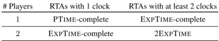
5.2 Computational complexity
All the results stated here concern glitch-free recursive timed automata only and their formal proofs can be found in [21]. First, we summarise the complexity results for the reachability problem for glitch-free RTAs in Table 2.
# Players RTAs with 1 clock RTAs with at least 2 clocks
1 PTIME-complete EXPTIME-complete
2 EXPTIME-complete 2EXPTIME
Table 2.Complexity results for glitch-free RTAs
By examining the reduction of RTAs to the corresponding RSMs via region abstraction in the previous section, it can be observed that in the case where all the clocks are passed by reference (i.e. they are global) only the number of internal nodes
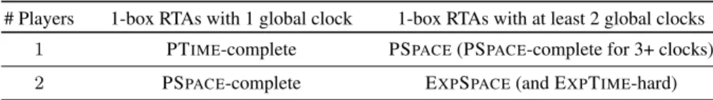
and exits grows exponentially, not the number of boxes. It is simply because the clocks values are never being restored to the value they had before the box was called and hence the valuation of the clocks does not have to be stored at the boxes in the region abstraction. This observation allows us to provide better complexity upper and lower bounds for the reachability problem and games on 1-box RTAs with global clocks, summarised in Table 3, because 1-box RSMs can be analysed a lot more efficiently than multi-exit RSMs. Since the number of exits can grow arbitrarily large after region abstraction is applied to a 1-exit RTA with just a single global clock, no similar improvement can be obtained for 1-exit RSMs with only global clocks.
# Players 1-box RTAs with 1 global clock 1-box RTAs with at least 2 global clocks
1 PTIME-complete PSPACE(PSPACE-complete for 3+ clocks)
2 PSPACE-complete EXPSPACE(and EXPTIME-hard)
Table 3.Complexity results for 1-box RTAs with only global clocks
On the other hand, if all clocks are local then only the number of boxes grows exponentially, not the number of control states (in particular the number of exit ports of each box does not increase). This allows us to provide a much better complexity upper and lower bounds for 1-exit RTAs with only local clocks. We summarise the results for the reachability problem for this subclass of RTAs in Table 4. Again, even if there is only one single local clock, the number of boxes can grow arbitrarily large after the region abstraction is applied to such a system, hence no similar improvements can be achieved when restricting the model to 1-box RTAs with local clocks.
# Players 1-exit RTAs with 1 local clock 1-exit RTAs with at least 2 local clocks
1 PTIME-complete EXPTIME-complete
2 PTIME-complete EXPTIME-complete
Table 4.Complexity results for 1-exit RTAs with only local clocks
6
Conclusion
We defined a natural extension of boolean programs with real-time clocks. These clocks, among others, may either correspond to physical time or other continuous values read from sensors. Just like in any advanced imperative programming language, we allow to pass these clocks by value or by reference. We showed that unfortunately arbitrary mixing of these two kinds of variable passing leads to undecidability. On the other hand, if we disallow it, the model becomes decidable and for many special subclasses of this model, the computational complexity is not higher than PSPACEfor 1 player setting and EXPTIMEfor 2 players setting, which is the same as the respective reachability analysis of ordinary finite-state timed automata.
Acknowledgment
References
1. R. Alur, M. Benedikt, K. Etessami, P. Godefroid, T. Reps, and M. Yannakakis. Analysis of recursive state machines. ACM Transactions on Programming Languages and Systems, 27:786–818, July 2005.
2. R. Alur and D. Dill. A theory of timed automata. InTheor. Comput. Sci., volume 126, 1994. 3. Rajeev Alur and Mihalis Yannakakis. Model checking of hierarchical state machines. In
ACM SIGSOFT’98, pages 175–188, 1998.
4. T. Ball and S. Rajamani. The slam toolkit. InInternational Conference on Computer Aided Verification, CAV 2001, pages 260–264, 2001.
5. A. Bouajjani, R. Echahed, and R. Robbana. On the automatic verification of systems with continuous variables and unbounded discrete data structures. InHybrid Systems II, volume 999 ofLNCS, pages 64–85, 1995.
6. Ahmed Bouajjani, Rachid Echahed, and Riadh Robbana. Verification of context-free timed systems using linear hybrid observers. In International Conference on Computer-Aided Verification, CAV’94, pages 118–131, 1994.
7. F. Bouchy, A. Finkel, and A. Sangnier. Reachability in timed counter systems. Electronic Notes in Theoretical Computer Science, 239:167 – 178, 2009. Proc. of 8th, 9th, and 10th Intl. Workshops on Verification of Infinite-State Systems (INFINITY 06, 07, 08).
8. Giorgio C. Buttazzo. Hard Real-time Computing Systems: Predictable Scheduling Algorithms And Applications. Springer-Verlag, Santa Clara, CA, USA, 2004.
9. Franck Cassez, Jan J. Jessen, Kim G. Larsen, Jean-Franc¸ois Raskin, and Pierre-Alain Reynier. Automatic synthesis of robust and optimal controllers — an industrial case study. InHSCC ’09, pages 90–104. Springer-Verlag, 2009.
10. Z. Dang. Binary reachability analysis of pushdown timed automata with dense clocks. In International Conference on Computer Aided Verification, CAV 2001, volume 2102 ofLNCS, pages 506–517. Springer, 2001.
11. Z. Dang. Pushdown timed automata: a binary reachability characterization and safety verification. Theor. Comput. Sci., 302(1-3):93–121, 2003.
12. Stephane Demri and Regis Gascon. The Effects of Bounding Syntactic Resources on Presburger LTL.J. Logic Computation, 19(6):1541–1575, 2009.
13. M. Emmi and R. Majumdar. Decision problems for the verification of real-time software. In Hybrid Systems: Computation and Control, pages 200–211, 2006.
14. K. Etessami and M. Yannakakis. Recursive markov decision processes and recursive stochastic games. InProc. ICALP’05, pages 891–903, 2005.
15. Kousha Etessami. Analysis of recursive game graphs using data flow equations. In VMCAI’04, pages 282–296, 2004.
16. S. Graf and H. Saidi. Construction of abstract state graphs with PVS. InCAV’97, pages 72–83, 1997.
17. Petr Jancar and Zdenek Sawa. A note on emptiness for alternating finite automata with a one-letter alphabet.Inf. Process. Lett., 104(5):164–167, 2007.
18. Dominik Wojtczak Kousha Etessami and Mihalis Yannakakis. Quasi-Birth-Death processes, Tree-like QBDs, Probabilistic 1-Counter Automata, and Pushdown Systems. Performance Evaluation, 67(9):837 – 857, 2010. Special Issue of QEST 2008.
19. Marvin L. Minsky.Computation: finite and infinite machines. Prentice-Hall, Inc., 1967. 20. Olivier Serre. Parity games played on transition graphs of one-counter processes. In
FoSSaCS’06, pages 337–351, 2006.
21. Ashutosh Trivedi and Dominik Wojtczak. Recursive timed automata. Oxford University Computing Laboratory technical report, RR-10-09, 2010.
22. Igor Walukiewicz. Pushdown processes: Games and model checking. In International Conference on Computer Aided Verification, CAV 1996, pages 62–74, 1996.
![Fig. 1. Example recursive state machine taken from [1]](https://thumb-us.123doks.com/thumbv2/123dok_us/978586.2628412/5.918.200.724.136.281/fig-example-recursive-state-machine-taken.webp)