Stock Return Predictability And Taylor Rules

Archived version from NCDOCKS Institutional Repository http://libres.uncg.edu/ir/asu/

Stock Return Predictability And Taylor Rules

By:

Onur Ince,

Lei Yu Jiang, and Tanya Molodtsova

Abstract

This paper evaluates stock return predictability with inflation and output gap, the variables that typically enter

the Federal Reserve Bank’s interest rate setting rule. We introduce Taylor rule fundamentals into the Fed model

that relates stock returns to earnings and long-term yields. Using real-time data from 1970 to 2008, we find

evidence that the Fed model with Taylor rule fundamentals performs better in-sample and out-of-sample than the

constant return and original Fed models. We evaluate economic significance of the stock return models and find

that the models with Taylor rule fundamentals consistently produce higher utility gains than the benchmark models.

Ince, O.

, Jiang, L.Y., & Molodtsova, T. (2016). Stock Return Predictability and Taylor Rules. Available at:

https://www.semanticscholar.org/paper/Stock-Return-Predictability-and-Taylor-Rules-Ince-Jiang/

fa4614302b9b466f5691af5c4735445f5e6d6947

Stock Return Predictability and Taylor Rules

Onur Ince

*

Lei Jiang

**

Tanya Molodtsova

***

November 14, 2016

Abstract

This paper evaluates stock return predictability with inflation and output gap, the variables that typically enter the Federal Reserve Bank’s interest rate setting rule. We introduce Taylor rule fundamentals into the Fed model that relates stock returns to earnings and long-term yields. Using real-time data from 1970 to 2008, we find evidence that the Fed model with Taylor rule fundamentals performs better in-sample and out-of-sample than the constant return and original Fed models. We evaluate economic significance of the stock return models and find that the models with Taylor rule fundamentals consistently produce higher utility gains than the benchmark models.

JEL Classification: G10, G11, G14, E44

Keywords: stock returns, predictability, Taylor rules

We thank Lutz Kilian, Richard Luger, Essie Maasoumi, Ellen Meade, Nicole Simpson, Elena Pesavento, Cesare Robotti, and participants at the 2010 Southern Economic Association Conference and the workshop at Auburn University for helpful comments and discussions. Special thanks to Jeff Racine for providing his R code and helpful suggestions.

*_{Department of Economics, Walker School of Business, Appalachian State University, Boone, NC, 28608. Tel: +1}

(828) 262-4033 Email: [email protected]

** _{Department of Finance, School of Economics and Management, Tsinghua University, Beijing, China, 100084. Tel:}

+86 (010) 62797084. Email: [email protected]

*** _{Department of Economics, Walker School of Business, Appalachian State University, Boone, NC, 28608. Tel: +1}

1. Introduction

Despite voluminous literature on stock return predictability, no definite conclusion has yet emerged as to whether stock returns are predictable with any financial and macroeconomic variables. While some studies find evidence of in-sample and/or out-of-sample stock return predictability, the results are not robust to the choice of the sample period and estimation methodology. Those studies that find evidence of stock return predictability with selected variables rarely attempt to explain what drives the relationship. A comprehensive study by Goyal and Welch (2008) summarizes the dismal state of the literature by concluding that none of the conventional macroeconomic or financial variables can predict excess returns in-sample or out-of-sample over the last 30 years.

Studying the links between monetary policy and asset prices is important for both the practitioners and policymakers. However, there is a significant disconnection between most empirical research on stock return predictability and the literature on monetary policy evaluation that is based on some variant of a Taylor (1993) rule. The idea that monetary policy decisions affect the stock market is widely accepted among the practitioners. From an investor’s point of view, understanding the relationship between the stock price behavior and monetary policy is important to gauge empirical asset pricing. Since the stock prices are determined in a forward-looking manner, monetary policy is likely to affect the stock prices through its influence on market participants’ expectations about the future economic activity, which, in turn, affect the determination of dividends and stock return premiums. Bernanke and Kuttner (2005) argue that “the most direct and immediate effects of monetary policy actions, such as changes in the federal funds rate, are on the financial markets; by affecting asset prices and returns, policymakers try to modify economic behavior in ways that will help to achieve their ultimate objectives.” Thus, exploring the links between monetary policy and asset prices is essential for policymakers to understand the monetary policy transmission mechanism.

An extensive literature has examined the relationship between business condition indicators and changes in stock prices directly. For example, Fama and Schwert (1977) document the negative effect of inflation shocks on the realized common stock returns. Cooper and Priestley (2008) find that the output gap is useful for predicting stock returns. Maio (2013) evaluates economic significance of trading strategies based on the federal funds rate (FFR), and finds the evidence of significant gains. Boyd et al. (2005) focus on the stock market’s response to employment news, and find that the stock prices rise when there is bad labor market news during expansions, and fall during contractions. Campbell and Vuolteenaho (2004) try to explain the negative relationship between inflation and expected stock returns in three potential ways: (1) inflation drives down the real dividend growth, (2) inflation drives up the risk premium, and (3) inflation illusion makes stock market participants fail to see that higher inflation should increase the nominal dividend growth.

In general, the connection between monetary policy and stock returns is examined in the literature either in a structural VAR framework or using event study methodology.1 _{This paper is different in two}

ways. First, we focus on the role of monetary policy for stock return predictability. Second, we explicitly introduce variables that determine the target interest rate in a monetary policy rule into the stock return predictive equation, which allows for richer dynamics than solely using the federal funds rate. A typical interest rate setting rule for the Federal Reserve Bank introduced by Taylor (1993) posits that the nominal interest rate responds to the inflation rate, the difference between inflation and its target, the output gap, the equilibrium real interest rate, and (in different variants of Taylor rule) the lagged interest rate and the real exchange rate. This simple rule has become the dominant method for evaluating monetary policy.2

In this paper, we connect business condition variables, such as the inflation and output gap, with stock returns via the monetary policy channels. In the setup of our model, we follow Asness (2003), who claims that inflation increases both the nominal interest rate and dividend growth, and assumes that the nominal earning growth is unrelated to inflation expectations. We also assume, as in Campbell and Vuolteenaho (2004), that the subjective risk premium of holding stocks over bonds is unrelated to inflation and constant over time. Therefore, the existence of a negative relationship between the inflation and expected stock return in our model is consistent with the inflation illusion argument. Brown et al. (2016) examine the cross-sectional relationship between stock returns and inflation and confirm the Modigliani and Cohn (1979) inflation illusion hypothesis.

In contrast with the previous literature that links stock returns and macroeconomic variables, we ask a different question by looking at the effect of Taylor rule fundamentals on the forecasted stock returns. Looking at the coefficients on inflation and output gap, we find that the output gap coefficient is negative throughout the entire sample with a sharp decline around 2000 and 2003. An increase in the U.S. inflation leads to a decrease in the forecasted stock returns over the entire sample. The Federal Reserve Bank responds to an increase in inflation by increasing the federal funds rate, which, in turn, increases earning-to-price ratio. Furthermore, changes in the interest rates cause stock market participants to rebalance their portfolios and generate a negative relationship between the inflation and expected stock returns.

1

For example, Patelis (1997), Thorbecke (1997), and Goto and Valkanov (2002) use VAR-based models to study

stock return response to changes in either the federal funds rates (FFR), inflation, or federal funds futures. Bernanke and Kuttner (2005) study the impact of monetary policy surprises on stock prices, and find that a 25-basis-point cut in the federal funds rate is associated with a one-percent increase in broad stock indexes. Crowder (2006) estimates the response of stock returns to innovations in the federal funds rate in a SVAR model that either includes or excludes price index, and finds that positive shocks in FFR leads to immediate declines in the S&P 500 returns and an increase in the price index leads to higher FFR and lower stock returns. Rigobon and Sack (2004) estimate the response of daily stock returns to changes in FFR in a GARCH model. D’Amico and Farka (2003) study the response to changes in federal funds futures on Federal Open Market Committee (FOMC) meeting days. Both papers conclude that monetary tightening leads to declines in equity returns.

2_{Asso, Kahn, and Leeson (2007) examine the history of the Taylor rule and its influence on macroeconomic research}

To our knowledge, this is the first paper to study the role of monetary policy for stock return predictability using Taylor rule fundamentals. Since investors form their expectations about the future monetary policy based on the variables in the Taylor rule, including the inflation and output gap in the stock return predictive regression allows us to capture market participants’ expectations about current and future monetary policy that drive the stock prices over and beyond the changes in the actual interest rate. Several recent papers connect exchange rates with market expectations using Taylor rules and find that the exchange rate models with Taylor rule fundamentals outperform the naïve no-change model and the conventional purchasing power parity, monetary, and interest rate models in out-of-sample comparisons.3

We use real-time data on inflation and real output to examine in-sample and out-of-sample predictability of monthly stock returns from 1970 to 2008. Real-time data, the data available to investors at the time the decisions were made, is crucial to mimic the decision-making process of stock market participants as closely as possible. The starting point of our analysis is the so-called Fed model that has originated in the annals of a Fed report, but is not officially endorsed by the Fed.4 _{The model posits that the}

stock returns are governed by earnings and nominal interest rate. Despite the Fed model’s satisfactory in-sample and out-of-in-sample performance, it does not reflect how the monetary policy is conducted or evaluated. We modify the Fed model by replacing interest rates with the Taylor rule fundamentals and call it the Fed model with Taylor rule fundamentals, as opposed to the original Fed model. If stock prices react mostly to market expectations about the future macroeconomic indicators, which are formed based on current Taylor rule fundamentals, incorporating real-time inflation and output gap estimates into the stock return model could improve its forecasting power. It is worth noting that we estimate rather than impose specific Taylor rule coefficients on inflation and output gap in the stock return forecasting equation.

We consider several specifications of the Fed model with Taylor rule fundamentals. In the simplest Taylor rule, the nominal interest rate responds to changes in inflation and output gap. Following Clarida, Gali, and Gertler (1998), it has become common practice to assume partial adjustment of the interest rate to its target within a period. To incorporate gradual adjustment of the federal funds rate to its target, we include lagged interest rate into the model in addition to the inflation rate and output gap. We call the model with Taylor rule fundamentals that includes the lagged interest rate the model with smoothing. Also, we consider the model with no smoothing that excludes the lagged interest rate. The Federal Open Market Committee (FOMC) meets every 6-8 weeks to set the target interest rate, and that target rate is gradually achieved over the next few months. Therefore, short-run forecasting power of stock return models could

3 _{See, for example, Engel, Mark, and West (2008), Ince (2014), Molodtsova and Papell (2009, 2013), Ince,}

Molodtsova, and Papell (2016), and Molodtsova, Nikolsko-Rzhevskyy, and Papell (2008, 2011).

4 _{The term “Fed model” was coined by a Prudential Securities strategist, Ed Yardeni, who plotted a time series for the}

earnings-price ratio of the S&P500 against the 10-year constant-maturity nominal treasury yield in the Federal Reserve Humphrey Hawkins Report for July 1997.

potentially be improved by including Taylor rule fundamentals that signal about future macroeconomic developments.

First, we begin by examining the in-sample performance of the Fed model with Taylor rule fundamentals using standard in-sample measures of fit. Overall, the in-sample fit of the Fed model with Taylor rule fundamentals is much stronger than that of the constant return and original Fed models. We then evaluate the out-of-sample performance of the model with Taylor rule fundamentals. In fact, as discussed in Inoue and Kilian (2004), in-sample predictability does not necessarily imply out-of-sample predictability, and vice versa. In addition to the comparisons based on the out-of-sample R-squared, defined as one minus the ratio of the mean squared prediction error (MSPE) from the Fed model with Taylor rule fundamentals to the MSPEs of the alternative models, the constant return and original Fed model, the out-of-sample predictability of stock return models is evaluated using two other test statistics that are based on the MSPE comparison, the Diebold and Mariano (1995) and West (1996) (DMW) test and the Clark and West (2006) (CW) test.

While the DMW test statistic is appropriate for testing equal predictability of two non-nested models, when comparing the MSPE’s of two nested models, the use of DMW test with standard normal critical values usually results in very poorly sized tests, with far too few rejections of the null.5 _McCracken

(2007) tabulated the asymptotic critical values that can be used for 1-step ahead forecast comparisons using the DMW test. However, as suggested in Rogoff and Stavrakeva (2008), we use bootstrapped critical values instead of relying on the critical values tabulated in McCracken (2007).6 _{The CW test adjusts the DMW}

statistic for nested-model comparisons. Although the simulations in Clark and West (2006) indicate that the inference made using asymptotically normal critical values typically results in properly sized tests, the inference based on bootstrapped critical values have higher power.7

Based on the DMW and CW statistics, we find strong evidence of stock return predictability for the Fed model with Taylor rule fundamentals, which is robust to different measures of economic activity and window sizes.8 _{Also, the Fed model with Taylor rule fundamentals outperforms the original Fed model,}

when most of the observations in the regression equation fall into the period where the Fed is generally characterized by a Taylor rule. This result suggests that Taylor rule fundamentals contain important predictive information for stock returns that cannot be obtained from the interest rates alone.

5 _{McCracken (2007) shows that using standard normal critical values for the DMW statistic results in severely}

undersized tests, with tests of nominal 0.10 size generally having actual size less than 0.02.

6 _{Both approaches produce nearly identical results.}

7 _{We bootstrap the critical values for CW test using the algorithm described in Section 4.}

8 _{Rogoff and Stavrakeva (2008) point out that the evidence of exchange rate predictability with CW and DMW}

statistics may not be consistent over different window sizes in rolling estimation scheme. Inoue and Rossi (2012) discuss the robustness of out-of-sample forecasting to the size of the forecast window. We use various window sizes to ensure the robustness of the results.

In addition to the out-of-sample tests that are based on the mean squared prediction error comparison, we use the Bhattacharya-Matusita-Hellinger metric entropy developed by Bhattacharya (1943), Matusita (1955), and Hellinger (1909) to test for the generic dependence of stock returns on Taylor rule fundamentals. The entropy measure is defined over densities of stock returns that are estimated non-parametrically following Maasoumi and Racine (2002). If the actual returns and the returns predicted by the Fed Model with Taylor rule fundamentals are independent, the value of this metric is zero. The value of the entropy measure increases as the model's predictive ability improves. Significant test statistics based on the Bhattacharya-Matusita-Hellinger test indicate that the stock returns depend on the predictors in the Taylor rule based model. Although we find significant nonparametric dependence with all three models, the performance of the Fed model with Taylor rule fundamentals is more robust to the choice of the window size than the performance of the constant return and the original Fed model.

Finally, we evaluate the economic significance of the Fed model with Taylor rule fundamentals. To determine whether a trading strategy based on the Fed model with Taylor rule fundamentals can generate higher utility gains than a strategy based on either the constant return or the original Fed model, we compare the certainty equivalence for these three models following the methodology in Ferreira and Santa-Clara (2011). We find substantial utility gains from timing the market using the Fed model with Taylor rule fundamentals. The models with Taylor rule fundamentals consistently produce higher utility gains than the two alternative models. This finding is also robust to the choice of the measure of economic activity and data frequency. Thus, including Taylor rule fundamentals into the Fed Model improves not only statistical, but also economic performance of the benchmark model.

The rest of the paper is organized as follows. Section 2 introduces the Fed Model with Taylor rule fundamentals that is estimated in-sample and used for out-of-sample model comparisons. In Section 3, we describe the data. Section 4 introduces the out-of-sample statistical and economic evaluation methodologies and describes how the inference is made. In Section 5, we discuss the empirical results of in-sample and out-of-sample tests. Section 6 concludes.

2. Stock Return Models

The starting point for our analysis is a simple model that became known as the Fed model, where stocks and bonds are competing for space in a representative investor’s portfolio. Following the adjustments made for the subjective risk premium of holding stocks versus bonds and the growth rate of dividends, the earnings to price ratio of a representative stock, or stock market index, should rise after an increase in the long-term bond yields. Otherwise, a decline in the earnings to price ratio could lead investors to invest in the bond market. In the equilibrium, the yield on stocks (earnings to price ratio) is correlated with the yield on bonds:

_t t t lty p e E _ 







     * (1)

where

lty

is the long term yield on a Treasury bond, and

t t p

e _{is the earnings to price ratio.}

Stock prices can be under- or overvalued and drive the observed earnings to price ratio away from the equilibrium. For instance, Lander, Orphanides and Douvogiannis (1997) show that portfolio adjustments between stocks and bonds make the stock prices move so that the difference between actual and equilibrium earnings to price ratio declines (given exogenous earnings). In the absence of dividends, the change in the stock return will be correlated with the deviation from equilibrium earnings to price ratio. For example, if  ( ) t t t t p e E p e

, a positive deviation indicates that the stock price is undervalued. Thus, investors would have an incentive to hold more stocks, which causes stock prices to rise in the next period and generates positive stock returns,

r

t₁:

₁ * 1 1 1                     _t t t t t t p e E p e r







(2) Substituting equation (1) into equation (2), yields

1







lty t



t1 t t d t

lty

p

e

r









(3) where







₁



₁,



_d 



₁, and



lty 



1



.

We refer to equation (3) as the original Fed model thereafter. This model has been found relatively successful in empirical in-sample and out-of-sample analysis. For example, Thomas and Zhang (2008) suggest using the Fed model in describing rational stock markets and providing insights about stock market valuation.

According to the pure expectation theory in Campbell (1987) and Fama and French (1989), we can replace the long-term bond yield in equation (3) with the sum of the term spread and federal funds rate,

₁







lty

(

t



t

)



t₁ t t d t

term

i

p

e

r









(4) where i_t is federal funds rate, and term_tis the term spread.9

9 _{Even though there is a possible bond risk premium term on the right-hand side of the equation, it is not possible to}

Following Taylor (1993), the monetary policy rule to be followed by the Fed is as follows: i_t* 



_t 



(



_t 



*)



y_t rer* (5) where i_t* is the target level of the federal funds rate,



_tis the inflation rate,



*is inflation target, y_t is the output gap, defined as percent deviation of actual output from its potential level, and

rer

*is the equilibrium level of the real interest rate.

We can combine



*and

rer

* in equation (5) into a constant term,





rer

*





*, which leads to the following equation for the target level of short-term nominal interest rate,

i

_t*









_t





y

_t

(6) where



1



.

Following Clarida, Gali and Gertler (1998), we allow for the possibility that the interest rate adjusts gradually to achieve its target level,

i

_t



(

1





)

i

_t*





i

_t1



v

_t (7) where 0



1. Substituting equation (6) into (7), yields,

i

t



(

1





)(







t





y

t

)





i

t1



v

t (8)

To derive the Fed model with Taylor rule fundamentals that is used for forecasting stock returns, we substitute equation (8) into equation (4),

1







t t



t



y t



i t1



t1 t t d t

term

y

i

p

e

r









_









(9) where







₁





₁,



d





1,



t







1



,











1



(

1





)



,



y







1



(

1





)



, and







i





1 .

If the interest rate adjusts to its target level within a period,



_i



0

, andthe Fed model with Taylor rule fundamentals without smoothing becomes,

1







t



t



y t



t1 t t d t

term

y

p

e

r









_







(10)

An increase in the inflation rate and/or output gap would cause the Federal Reserve to increase the federal funds rate to stabilize the economy. Also, an increase in the federal funds rate pushes the implicit equilibrium yield in the stock market up and generates a deviation between the observed and equilibrium yield. In the next period, the stock prices are expected to decrease to move the yield back towards the equilibrium, which decreases the expected price change or causes a negative expected return.

3. Data

We use monthly data starting from February 1970, the earliest date for which all the variables used in our analysis are available, until November 2008 for the U.S. The end of the sample period is chosen to correspond with (1) the onset of the financial crisis of 2008-2009 and (2) the approximate start of the period when the federal funds rates were effectively at the zero lower bound. Since the objective of the paper is to assess the role of the conventional monetary policy for stock return predictability, the unconventional monetary policy era of post-2008 period is outside of the scope of this study.

The stock return is continuously compounded return on the S&P500 index including dividends obtained from the Center for Research in Security Prices (CRSP). The long term yield on government bond, end-of-month S&P500 index, and moving sum of 12-month earnings on the S&P 500 index are from Amit Goyal’s website.10 _{Term spread is the difference between the long term yield and the federal funds rate.}

Earnings to price ratio is the ratio of earnings to S&P500 index. The federal funds rate is taken from the Federal Reserve Bank of St. Louis (FRED) Database.

The real-time prices and seasonally adjusted industrial production index are from the Philadelphia Fed Real-Time Database for Macroeconomists described in Croushore and Stark (2001). The real-time dataset has standard triangular format with the vintage dates on the horizontal axis and calendar dates on the vertical axis. The term vintage is used to denote each date for which we have data as they were observed at the time. The real-time data is constructed from the diagonal elements of the real-time data matrix by pairing vintage dates with the last available observations in each vintage. This type of data is referred to as the first-release data, as opposed to the current-vintage data that uses all the information in each vintage, so that the data is fully updated each period. The advantage of using the first-release data is that it reflects market reaction to news about macroeconomic fundamentals. While the first-release data has been used before to examine foreign exchange rate predictability by Molodtsova, Nikolsko-Rzhevskyy, and Papell (2008) and Ince (2014), it has not been explored in the literature on stock return predictability.

The GDP Deflator is used to measure the overall price level in the U.S. economy. The inflation rate is the annual inflation rate calculated using the log difference of the GDP Deflator (the last available observation in monthly vintages) over the previous 12 months. The index of seasonally adjusted industrial production is used to measure the level of output. The output gap depends on the estimate of potential output, a latent variable that is frequently subject to ex-post revisions. Since there is no consensus about which definition of potential output is used by central banks or the public, we follow Ince and Papell (2013) and estimate the output gap as percentage deviations of actual output from a linear time trend, quadratic time trend, Hodrick-Prescott (1997) (HP) trend, and Baxter and King (1999) (BK) trend.11 _{To take into}

10 _{http://www.hec.unil.ch/agoyal/}

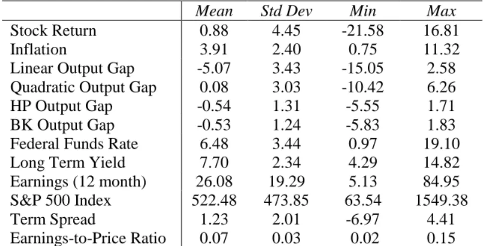
account the end-of-sample uncertainty in the estimation of the HP and BK filters, which becomes even more severe with real-time data when no future data is available and the focus is on the last available observation in each period, we apply the technique proposed by Watson (2007). We use AR (8) model to forecast and backcast the industrial production growth 12-periods ahead before applying the HP and BK filters. The descriptive statistics for the variables are presented in Table 1.

4. Model Comparisons

4.1 MSPE-Based Out-of-Sample Predictability Tests

The central question in this paper is whether the variables that typically enter a Taylor rule can provide evidence of out-of-sample predictability for stock returns. To evaluate the out-of-sample performance of the models with Taylor rule fundamentals, we use two test statistics that are based on the MSPE comparison: the Diebold and Mariano (1995) and West (1996) (DMW) test and the Clark and West (2006). The two tests are described below.

Following much of the literature on stock return predictability, we first compare the out-of-sample performance of the Fed model with Taylor rule fundamentals in equations (9) and (10) to that of the constant return model, which serves as a standard benchmark model in the literature. In this case, we are interested in comparing the mean square prediction errors from two nested models:

Model 1:

y

_t









_t

Model 2:

y

_t



X

_t'







_t, where

E

_t1

(



_t

)



0

The simplest statistic that is commonly used in the literature to compare the out-of-sample performance of the two models is the out-of-sample 2,

R which is defined as follows,

1 2 2

1

MSPE

MSPE

R

OOS







(11) where

MSPE

₁ and

MSPE

₂ are the mean squared prediction errors from the constant return model and the Fed model with Taylor rule fundamentals, respectively. Therefore, when the MSPE of the Fed model with Taylor rule fundamentals is smaller than that of the constant return model, the out-of-sampleR2is positive, which presents evidence in favor of the Fed model with Taylor rule fundamentals.

To formally test the null hypothesis that the two MSPEs are equal against the alternative that the MSPE of Model 2 is smaller than that of Model 1, we apply the test introduced by Diebold and Mariano (1995) and West (1996) that uses the sample MSPEs to construct a t-type statistic, which is assumed to be asymptotically normal. To construct the DMW statistic, let

22, 2 , 1

ˆ

ˆ

ˆ

t t t

e

e

f





and



    







T P T t t

f

P

f

1 2 2 2 1 1 1

ˆ



ˆ



ˆ

,

where eˆ1,_tand

e

ˆ

2,t are the sample forecast errors from Models 1 and 2, respectively. Then, the DMW test

statistic is computed as follows,

V

P

f

DMW

ˆ

1 



, where



    





T P T t t

f

f

P

V

1 2 1 1

)

ˆ

(

ˆ

₍₁₂₎

Suppose we have a sample of T+1 observations. The last P observations are used for predictions. The first prediction is made for the observation R+1, the next for R+2, …, and the final for T+1. We have

T+1=R+P, where R is the size of rolling window, and P the total number of forecasts. To generate prediction for period t=R+1, …, T, we use only the information available prior to t.

McCracken (2007) shows that application of the DMW statistic with standard normal critical values to nested model comparisons results in severely undersized tests, which in our case would lead to far too few rejections of the null hypothesis of no predictability. Clark and West (2006) demonstrate analytically that the asymptotic distributions of sample and population difference between the two MSPEs are not identical, namely the sample difference between the two MSPEs is biased downward from zero under the null. To test for predictability, we construct the adjusted test statistic as described in Clark and West (2006). The CW statistic is calculated by correcting the sample MSPE from the alternative model by the amount of the bias. This adjusted CW test statistic is asymptotically standard normal.

After comparing the Fed model with Taylor rule fundamentals to the constant return model, we assess whether introducing inflation and output gap into the original Fed model in equation (3) helps to improve its out-of-sample predictability. In this case, the original Fed model and the Fed model with Taylor rule fundamentals are non-nested, and we can use the DMW test statistics. Instead of relying on the inference based on the asymptotic critical values for the DMW test provided in McCracken (2007), we bootstrap the critical values using the procedure suggested by Mark (1995), Kilian (1999) and Rapach and Wohar (2006). We first estimate the residuals for the regressions of (1) the stock return on a constant and (2) the Taylor rule fundamentals on its lagged values under the null hypothesis of no predictability. We then store the residuals and simulate the sequences of left-hand side variables by randomly drawing residual pairs with replacement to keep the contemporaneous correlation between the disturbances. We drop the first 100 observations and use the remaining observations for rolling regressions and calculate the DMW and CW statistics. We repeat the above-mentioned process 1000 times and obtain empirical distribution for the out-of-sample test statistics.

We use rolling estimation scheme to allow for more flexibility in the presence of possible structural breaks or time-varying coefficients. Rogoff and Stavrakeva (2008) point out that the evidence of exchange rate predictability with CW and DMW statistics may not be consistent over different window sizes. Similarly, Inoue and Rossi (2012) question the robustness of out-of-sample forecasts to the choice of the

forecast window. To avoid selecting a window size ad-hoc, we report the results using five different rolling window sizes with forecast starting in 1983:M3, 1986:M6, 1989:M9, 1991:M11, and 1994:M8 associated with 156-, 195-, 234-, 260-, and 293-month rolling windows starting from February 1970.12

4.2 Entropy-Based Nonparametric Dependence Tests

To ascertain the possibility of nonparametric relationship between stock returns and monetary policy variables, we use Bhattacharya-Matusita-Hellinger (BMH) metric entropy measure of non-parametric dependence. The BMH test is used to evaluate the nonnon-parametric dependence between distributions of actual and predicted returns from the competing models: the constant return model, the original Fed model, and the Fed model with Taylor rule fundamentals. The entropy measure allows for a generic, and possibly nonlinear, dependence of actual stock returns on their predictions that originate from the stock return models.

To calculate the BMH metric entropy measure, we estimate the stock return densities non-parametrically following Maasoumi and Racine (2002). If the actual and predicted returns are independent, the BMH metric is not significantly different from zero. The test statistic varies between zero and one and increases as the dependence between actual and forecasted stock returns becomes stronger. The entropy measure is calculated using the formula,

S

f

rr

f

r

f

r

drd

r

ˆ

2

1

2 2 1 ˆ 2 1 2 1 ˆ ,



  

















 (13)

where f_r,_rˆ is the joint density of stock returns and predicted returns,

f

r is the marginal density of stock

returns, and

f

_rˆ is the marginal density of predicted returns.

To test for the dependence between two distributions, the entropy measure uses the information about the entire distribution of actual and predicted stock returns rather than focusing on just the first two moments. The null hypothesis is the independence of the two distributions. An insignificant statistic indicates the failure of the model rather than simply the absence of correlation between the two distributions, which means that no significant information about stock return distribution is contained in the predictive equation.

Following Maasoumi and Racine (2002), we use kernel density estimator for the density of marginal and joint distributions of actual and predicted returns. The kernel function is the second order Gaussian kernel, where the bandwidth is selected via likelihood cross-validation. To calculate the critical values, we bootstrap the statistic under the null of independence. First, we perform the test for nonparametric dependence for the Fed model with Taylor rule model with and without interest rate smoothing. To

determine whether the Taylor rule fundamentals contain more predictive information for the actual stock returns, we repeat the nonparametric tests for the original Fed model and the constant return model and compare the results.

4.3 Economic Significance Tests

To test whether the trading strategy based on the Fed model with Taylor rule fundamentals can generate greater economic gains than the strategies based on the constant return and original Fed models, we follow Ferreira and Santa-Clara (2011) and compare the certainty equivalence from the competing models.13

Suppose that the utility function of a single period representative investor, U(Wt+1), is strictly

increasing and twice differentiable, and Wt+1 is the wealth level at time t+1. Since Et[U(Wt+1)] = U(CE),

where CE stands for the certainty equivalence, maximizing the expected utility is equivalent to maximizing the certainty equivalence with a strictly increasing utility function,

 

₁

 

₁

2 

 

Et Wt Vart Wt

CE



(14) which is derived from the Taylor approximation. We assume that the initial wealth is 1, and the coefficient of relative risk aversion equals .

If investors can invest either in a stock or in a risk-free asset,

W

t₁



w

t

r

t₁



(

1



w

t

)

rf

t₁ (15)

where

w

_t is the weight of stocks in the portfolio, rt+1is the stock return, and rft+1is the return on a risk-free

asset at time t+1, which is known at time t. To find the weight in the optimal portfolio for an investor, we

maximize the certainty equivalence. The optimal weight,

)

(

₁ 1 1   





t t t t t t

r

Var

rf

r

E

w



, is empirically estimated by

)

(

ˆ

ˆ

1 1 1   





t t t t

r

r

Va

rf

r

w



, where rˆt1 is the predicted value of stock return from the constant return model, the

original Fed model, or the Fed model with Taylor rule fundamentals, Varˆ(rt1) is the estimated variance

of stock return, and the risk-aversion parameter,, can take on the values of 1, 2, or 3. After the portfolio weight is determined, both the return and certainty equivalence is estimated for each model.

5. Empirical Results

We evaluate the in-sample and out-of-sample stock return predictability with Taylor rule fundamentals from February 1970 to November 2008. In addition to assessing the performance of the

13 _{Maio (2013) evaluates the economic significance of trading strategies based on the federal funds rate and finds the}

candidate models with parametric tests, we estimate the Bhattacharya-Matusita-Hellinger (BMH) metric entropy to test for the generic and non-parametric dependence of stock returns on predictive models. Finally, we evaluate the economic gains from using a trading strategy based on the competing models. The Fed model with Taylor rule fundamentals is estimated with and without the lagged interest rate using four different measures of the output gap. To ensure robustness of the results to the choice of the estimation window, we report the results using five different window sizes with initial forecasts starting in 1983:M3, 1986:M6, 1989:M9, 1991:M11, and 1994:M8.

5.1 In-Sample Estimation Results

We use the Generalized Method of Moments (GMM) estimator of Hansen (1982) to estimate the coefficients of the Fed model with Taylor rule fundamentals. GMM is relatively more successful in correcting the standard errors, and thus produces more efficient parameter estimates. We use the two-step efficient GMM estimator to obtain a consistent estimate of the weight matrix. In the first step, we estimate the parameters by specifying a weight matrix, which assumes that the moment conditions are independent and identically distributed. Then we apply the optimal bandwidth selection procedure suggested by Newey and West (1994) in the Bartlett kernel and compute a new heteroscedasticity and autocorrelation consistent (HAC) weight matrix. In the second step, we re-estimate the parameters using the new HAC consistent weight matrix. The instrumental variables that are chosen to satisfy the orthogonality conditions include the lagged values of right-hand side variables and the long term yield on the U.S. government bonds. To check whether the instruments satisfy the orthogonality conditions, we employ the J-test for overidentifying restrictions proposed by Hansen (1982). The J-statistic is distributed as χ2 with the degrees of freedom equal to the number of overidentifying restrictions. A rejection of the null hypothesis implies that one or more of the instruments do not satisfy the orthogonality conditions.

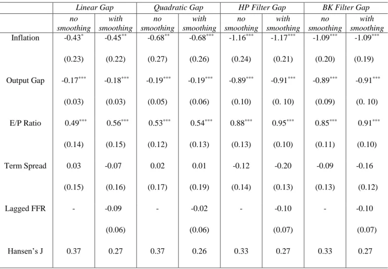
Table 2 displays the in-sample GMM estimates for the Fed model with Taylor rule fundamentals with and without the lagged interest rates (smoothing vs. no smoothing). For each model, we use four different measures of the output gap. We report the estimated coefficients on the inflation, output gap, earnings-to-price ratio, term spread, and lagged interest rate. The p-values for the J-test for each regression are presented in the last row.

The estimates of the inflation coefficients are negative and statistically significant for all 8 specifications. The output gap coefficients are also negative and significantly different from zero at the 1% level. Thus, as the inflation and/or output gap increase, the forecasted stock returns decrease. Although the coefficients on the lagged federal funds rate are not significant, they are also negative as expected. The J-statistics show that the chosen instruments for the right-hand side variables in the Fed model with Taylor rule fundamentals satisfy the orthogonality conditions.

To further assess the in-sample fit of the models, Table 3 presents the results for the R-squared, adjusted R-squared and root mean-squared errors (RMSE). The R-squared and adjusted R-squared for the Fed model with Taylor rule fundamentals are much higher in comparison with the benchmark models. Also, the in-sample predictions of the models with Taylor rule fundamentals produce lower RMSEs. Based on the in-sample fit criteria, the evidence suggests that the model with Taylor rule fundamentals outperforms both benchmark models.14

The in-sample analysis also provides supporting evidence for the inflation illusion hypothesis. Modigliani and Cohn (1979) assert that stock market investors fail to adjust their expectations for nominal dividend growth to match the rising long-term discount rate due to higher nominal interest rate, which leads to stock market underpricing during high inflation and to overpricing during low inflation periods. If there would be no significant relationship between inflation and stock return, this would support the claim in Asness (2003) that inflation increases both nominal interest rate and dividend growth at the same level and the effect of inflation on stock returns should be zero. Campbell and Vuolteenaho (2004) discuss the potential reasons for the negative relationship between inflation and stock return, and confirm the Modigliani and Cohn’s (1979) inflation illusion hypothesis. Overall, we find strong evidence to support the inflation illusion theorem. As shown in Table 2, inflation is negatively correlated with the future stock returns, regardless of which specification and measure of economic activity is used.

5.2 MSPE-Based Out-of-Sample Predictability Tests

As shown in Inoue and Kilian (2004), strong in-sample performance does not necessarily imply strong out-of-sample performance of the model, and vice versa. Thus, we compare the out-of-sample performance of the Fed model with Taylor rule fundamentals with that of the constant return and original Fed model. Unlike most of the previous studies that use the revised data on macroeconomic variables, we use real-time data on inflation and output gap that were available to investors when forecasts were made.

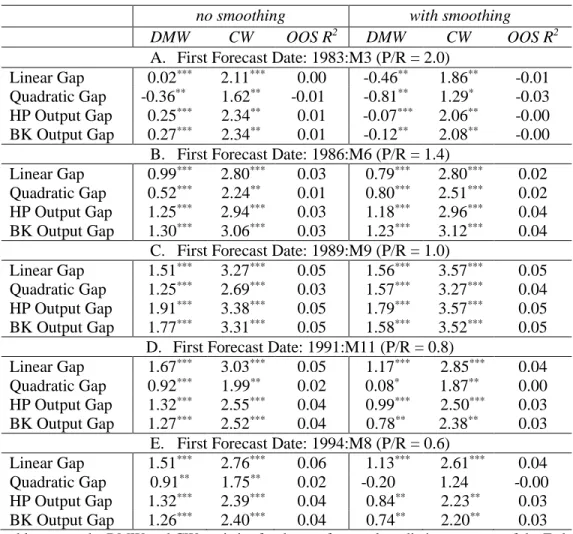
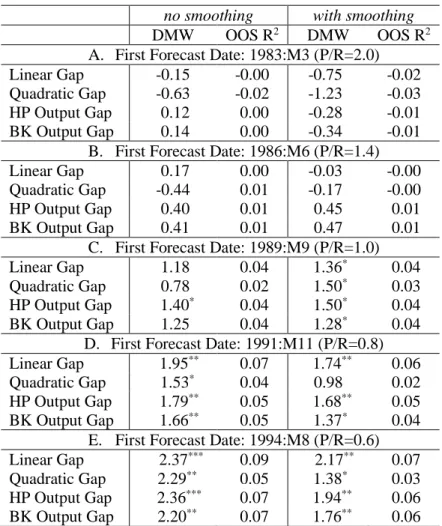
Table 4 reports the results for one-month ahead out-of-sample comparisons between the Fed model with Taylor rule fundamentals and the constant return model. We use four different measures of economic activity to estimate the output gap in the Fed model with Taylor rule fundamentals and five different window sizes. Since the two models are nested, we report both the DMW and CW statistics with bootstrapped critical values. Three observations can be made based on the results. First, there is strong evidence of stock return predictability with the Taylor-rule based specifications. Second, the evidence of stock return predictability is stronger with Taylor rule fundamentals with no smoothing than with smoothing

14

The results using quarterly instead of monthly data are qualitatively similar and available from the authors upon

request. In an unreported table, we estimate the equation (9) and (10) without the term spread. The results provide similar evidence in support of the Taylor rule based models.

based on all three statistics, the DMW, CW, and the OOS-R2_{. Third, the evidence of predictability with}

Taylor rule fundamentals with no smoothing are significant at least at the 5% level and robust to the choice of output gap estimates and rolling window sizes.

Having established that the Fed model with Taylor rule fundamentals outperforms the naïve constant return benchmark, the question remains about its relative out-of-sample performance with respect to the original Fed model. Since the model including Taylor rule fundamentals was derived from the original Fed model, it is unclear whether the Taylor rule fundamentals contain more predictive information about the stock returns than the Fed model.

Table 5 presents the results of out-of-sample tests for the null of equal predictability between the two models. In this case, the two models are non-nested and the DMW test can be used with standard normal critical values. The Fed model with Taylor rule fundamentals outperforms the original Fed model when the initial forecast starts in 1989. This period coincides with the Great Moderation, the period of significant decline in overall macroeconomic volatility (including lower volatility of inflation and output) since the mid-1980s, where the U.S. monetary policy is successfully characterized by a variant of the Taylor rule. The Fed model with Taylor rule fundamentals outperforms the original Fed model with at least one measure of the output gap for window sizes with the first forecast dates in September 1989, November 1991, and August 1994. Since most of the empirical evidence is consistent with the hypothesis that the Fed adopted some variant of the Taylor rule starting in the mid-1980s, our findings indicate that Taylor rule fundamentals contain additional predictive information for stock returns.

Panels C-E of Table 5 show that the model with interest rate smoothing performs better than the model with no smoothing between the 2nd _{quarter of 1986 and the 3}rd _{quarter of 1989, the period with}

relatively higher macroeconomic volatility than the post-1990 period. This result is reasonable as the main channels of monetary policy transmission, such as the interest rates, might be subject to inertia and might adjust gradually. Since November 1991, the model without smoothing significantly outperforms the original Fed model in all cases, and the model with smoothing outperforms the original Fed model in 7 out of 8 cases at least at the 10 percent level.

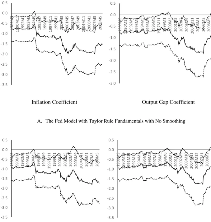
Finally, we present the time series dynamics of the coefficients on inflation and HP-filtered output gap for the two Taylor rule models with the first forecast date in September

1989

in Figure 1. The estimates of the inflation coefficients show that an increase in the U.S. inflation leads to a decrease in the forecasted stock returns over the entire sample. Similarly, the output gap coefficients are also negative throughout the entire sample with a sharp decline between 2000 and 2007. The coefficients follow similar pattern

regardless of how potential output is calculated.15 _{Our findings indicate that an increase in inflation and/or}

output gap causes a forecasted decrease in stock returns.

5.3 Entropy-Based Nonparametric Dependence Tests

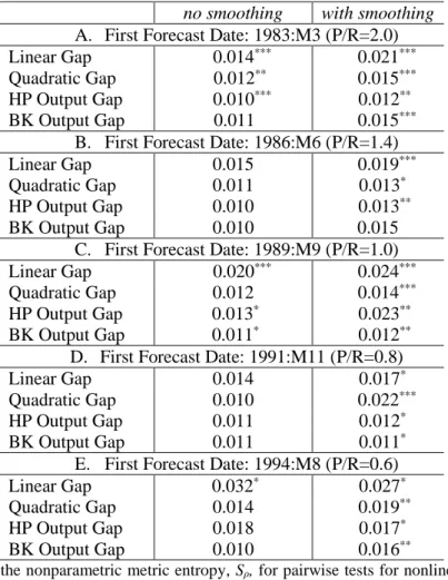
To relax the assumption of parametric dependence of stock returns on Taylor rule fundamentals, we test for the generic dependence of stock returns on Taylor rule fundamentals using the Bhattacharya-Matusita-Hellinger (BMH) metric entropy. Table 6 reports the results of the entropy-based dependence tests for the Fed model with Taylor rule fundamentals, and Table 7 contains the results for the two benchmark models. The entropy measure is defined over densities of stock returns that are estimated non-parametrically following Maasoumi and Racine (2002). If the actual returns and the returns predicted by the Fed Model with Taylor rule fundamentals are independent, the value of the BMH statistic is zero. The test statistic increases, as the model's predictive ability improves. A significant test statistic indicates that the stock return depends on the predictors in the Taylor rule model.

Across the specifications with and without smoothing, we find evidence of nonparametric dependence between the distribution of actual returns and predicted returns from the Taylor rule based models for all forecast windows with at least one measure of output gap. The strongest evidence of nonparametric dependence is found for the model with smoothing, where the BMH test is significant for all window sizes and output gap measures, with one exception for the BK output gap.

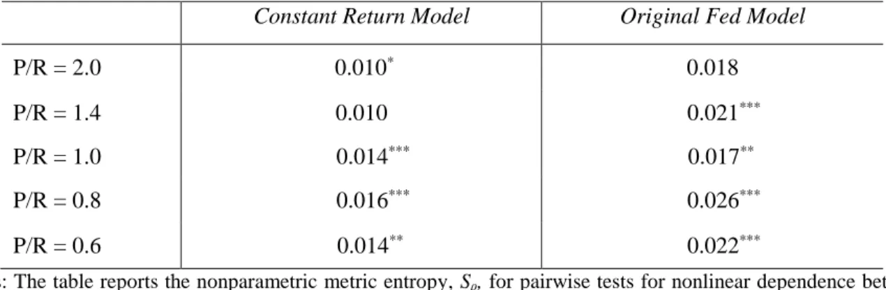
The results for the two benchmark models in Table 7 are less consistent across the choice of the forecast window. Significant evidence of nonparametric dependence is found for both models with 4 out of 5 window sizes. Although significant nonparametric dependence can be found with all three models, the results for the Fed model with Taylor rule fundamentals are more consistent across different window sizes.

5.4 Economic Significance Tests

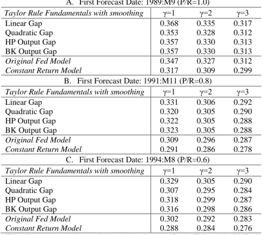
In addition to analyzing the predictive performance of the models using statistical measures, we evaluate their economic significance to determine whether a trading strategy based on the Fed model with Taylor rule fundamentals can generate higher utility gains than a strategy based on the constant return or the original Fed model. To do that, we focus on the periods where the Fed model with Taylor rule fundamentals outperforms the benchmark models (the periods with initial forecast dates in September 1989, November 1991, and August 1994), and compare the certainty equivalence for the best performing specification, the Taylor rule model with smoothing, against the two benchmark models.

Table 8 reports the certainty equivalence values for three different risk aversion parameters and three estimations windows described above. Each panel contains the results of certainty equivalence estimation for the Fed model with Taylor rule fundamentals with smoothing, the constant return model, and

the original Fed model. Two observations are apparent from the results. First, the original Fed model produces higher utility gains than the constant return model. Second, the Taylor rule based models consistently generate higher certainty equivalence statistics than the two benchmark models. The only exception from this pattern occurs for the Fed model with Taylor rule fundamentals and smoothing, when the economic activity is measured using the quadratic output gap. At the highest degree of risk aversion, the economic significance of this model is the same as the original Fed model when the first forecast starts in September 1989.

Overall, there is a strong evidence of substantial utility gains from timing the market using the Fed model with Taylor rule fundamentals. The finding of superior economic significance of the models with Taylor rule fundamentals is robust to the choice of the output gap measure and the forecast window. This result indicates that the market participants are using the information contained in inflation and output gap to generate positive profits, and trading strategies that are based on the Fed model with Taylor rule fundamentals can generate greater economic gains than trading strategies that are based on the constant return and Fed models. Thus, we find support for the hypothesis that including Taylor rule fundamentals improves economic, as well as statistical performance of the benchmark models.

6. Conclusions

Voluminous research on stock return predictability has not yet resolved the question of whether the stock returns are predictable and which variables can help to improve their forecasts. To examine the role of monetary policy for stock return predictability, we introduce the inflation and output gap, the variables that typically enter the Taylor rule, into the Fed model that relates stock returns to earnings and long-term yields. Using real-time data from 1970 to 2008, we evaluate in-sample and out-of-sample stock return predictability with Taylor-rule based models. The in-sample fit is much stronger for the Fed model with Taylor rule fundamentals than for the constant return or original Fed models. Since in-sample fit does not necessarily imply that the model can predict stock returns out-of-sample, we use parametric and non-parametric out-of-sample tests to compare the model with Taylor rule fundamentals with the two alternative benchmark models.

Based on the DMW and CW tests, we find strong evidence of out-of-sample stock return predictability with the Fed model with Taylor rule fundamentals, which is robust to the use of various measures of economic activity and different window sizes. The Fed model with Taylor rule fundamentals outperforms (1) the constant return model for all window sizes and (2) the original Fed model when most of the observations in the forecasting regression fall into the period when the U.S. monetary policy is generally characterized by a variant of Taylor rule. The dynamics of the estimated coefficients in the stock market forecasting equation indicates that an increase in inflation and/or output gap leads to a decrease in the forecasted stock returns. In addition to the out-of-sample predictability tests that are based on the mean

squared prediction error comparison, we use the Bhattacharya-Matusita-Hellinger metric entropy to test for the nonparametric dependence of stock returns on Taylor rule fundamentals. The dependence tests show that the Fed model with Taylor rule fundamentals produces results that are more consistent across different window sizes than the two alternatives.

Finally, we evaluate the economic significance of a trading strategy based on the Fed model with Taylor rule fundamentals, and find that it generates higher utility gains than the strategies based on the constant return or original Fed models. Among the two benchmark models, the Fed model produces greater economic gains than the constant return models. These findings are robust to the choice of the measure of economic activity and forecast window size. Therefore, we find evidence that the market participants are using the information contained in inflation and output gap to generate positive economic gains that are greater than the economic gains associated with the constant return and Fed models. Overall, we find strong support for the hypothesis that including Taylor rule fundamentals improves both statistical and economic performance of the benchmark models.

References

Asness, C., 2003. Fight the Fed Model: The Relationship between Future Returns and Stock and Bond Market Yields. Journal of Portfolio Management 30, 11-24.

Asso, F., Kahn, G., Leeson, R., 2007. The Taylor Rule and the Transformation of Monetary Policy. Federal Reserve Bank of Kansas City RWP 07-11.

Baxter, M., King, R., 1999. Measuring Business Cycles: Approximate Band-Pass Filters for Economic Time Series. Review of Economics and Statistics 81, 585–593.

Bernanke, B., Kuttner, K., 2005. What Explains the Stock Market's Reaction to Federal Reserve Policy? Journal of Finance 60, 1221-1257.

Bhattacharyya, A.,1943. On a Measure of Divergence between Two Statistical Populations Defined by Their Probability Distribution. Bulletin of the Calcutta Mathematical Society 35, 99-110.

Boyd, J., Hu, J., Jagannathan R., 2005. The Stock Markets’ Reaction to Unemployment News: Why Bad News Is Usually Good for Stocks. Journal of Finance 60, 649-672.

Brown, D. O., Huang D., Wang, F., 2016. Inflation Illusion and Stock Returns. Journal of Empirical Finance 35, 14-24.

Campbell, J., 1987. Stock Returns and the Term Structure. Journal of Financial Economics 18, 373–399. Campbell, J., Vuolteenaho, T., 2004. Inflation Illusion and Stock Prices. American Economic Review 94, 19-23.

Clarida, R., Gali J., Gertler, M., 1998. Monetary Rules in Practice: Some International Evidence. European Economic Review 42, 1033-1067.

Clark, T., West K., 2006. Using Out-of-Sample Mean Squared Prediction Errors to Test the Martingale Difference Hypothesis. Journal of Econometrics 135, 155-186.

Cooper, I., Priestley R., 2008. Time-Varying Risk Premiums and the Output Gap. Review of Financial Studies 22, 2801-2833.

Croushore, D., Stark T., 2001. A Real-Time Data Set for Macroeconomists. Journal of Econometrics 105, 111-130.

Crowder, W., 2006. The Interaction of Monetary Policy and Stock Returns. Journal of Financial Research 29, 523-535.

D’Amico, S., Farka, M., 2003. The Fed and Stock Market: A Proxy and Instrumental Variable Identification. Manuscript, Columbia University.

Diebold, F., Mariano R, 1995. Comparing Predictive Accuracy. Journal of Business and Economic Statistics 13, 253-263.

Engel, C., Mark N., West K., Exchange Rate Models Are Not as Bad as You Think. NBER Macroeconomics Annual 2007, 381-441.

Fama, E., French K., 1989. Business Conditions and Expected Returns on Stocks and Bonds. Journal of Financial Economics 25, 23–49.

Fama, E., Schwert G.W., 1977. Asset Returns and Inflation. Journal of Financial Economics 5, 115-146. Ferreira, M. Santa-Clara, P., 2011. Forecasting Stock Market Returns: The Sum of the Parts is more than the Whole. Journal of Financial Economics 100, 514-537.

Goto, S., Valkanov R., 2002. The Fed’s Effect on Excess Returns and Inflation is Bigger than You Think. Working paper, Anderson School of Management, University of California, Los Angeles.

Goyal, A., Welch I., 2008. A Comprehensive Look at the Empirical Performance of Equity Premium Prediction. Review of Financial Studies 21, 1455-1508.

Hellinger, E., 1909. Neue begr undung der theorie der quadratischen formen von unendlichen vielen ver anderlichen. Journal für die Reine und Angewandte Mathematik 136, 210–271.

Hodrick, R., Prescott, E., 1997. Postwar U.S. Business Cycles: An Empirical Investigation. Journal of Money, Credit, and Banking 29, 1-16.

Ince, O., 2014. Forecasting Exchange Rates Out-of-Sample with Panel Methods and Real-Time Data. Journal of International Money and Finance 43, 1-18.

Ince, O., Molodtsova T., and Papell D.H., 2016. Taylor Rule Deviations and Out-of-Sample Exchange Rate Predictability. forthcoming, Journal of International Money and Finance.

Ince, O., Papell D.H., 2013. The (Un)Reliability of Real-Time Output Gap Estimates with Revised Data. Economic Modelling 33, 713-721.

Inoue, A., Kilian, L., 2004. In-Sample or Out-of-Sample Tests of Predictability: Which One Should We Use? Econometric Reviews 23, 371-402.

Inoue, A., Rossi, B. 2012. Out-of-Sample Forecast Tests Robust to the Window Size Choice. Journal of Business and Economic Statistics 30, 432-453.

Kilian, L., 1999. Exchange Rates and Monetary Fundamentals: What Do We Learn from Long-Horizon Regressions? Journal of Applied Econometrics 14, 491-510.

Lander, J., Orphanides, A., Douvogiannis, M., 1997. Earnings, Forecasts and the Predictability of Stock Returns: Evidence from Trading the S&P. Journal of Portfolio Management 23, 24-35.

Maasoumi, E., Racine, J., 2002. Entropy and Predictability of Stock Market Returns. Journal of Econometrics 107, 291-312.

Maio, P., 2013. The “Fed Model” and the Predictability of Stock Returns. Review of Finance 17, 1489-1533.

Mark, N., 1995. Exchange Rates and Fundamentals: Evidence on Long-Horizon Predictability. American Economic Review 85, 201–218.

Matusita, K., 1955. Decision Rules Based on Distance for Problems of Fit, Two Samples and Estimation. Annals of Mathematical Statistics 26, 631–641.

McCracken, M., 2007. Asymptotics for Out of Sample Tests of Granger Causality. Journal of Econometrics 140, 719–752.

Modigliani, F., Cohn, R., 1979. Inflation, Rational Valuation, and the Market. Financial Analysts Journal, XXXV, 24-44.

Molodtsova, T., Nikolsko-Rzhevskyy A., Papell D.H., 2008. Taylor Rules with Real-Time Data: A Tale of Two Countries and One Exchange Rate. Journal of Monetary Economics 55, S63-S79

__________, 2011. Taylor Rules and the Euro. Journal of Money, Credit, and Banking 43, 535-552. Molodtsova, T., Papell D.H., 2009. Out-of-sample Exchange Rate Predictability with Taylor Rule Fundamentals. Journal of International Economics 77, 167-180.

__________, 2013. Taylor Rule Exchange Rate Forecasting during the Financial Crisis. NBER International Seminar on Macroeconomics 2012 9, 55-97.

Patelis, A., 1997. Stock Return Predictability and the Role of Monetary Policy. Journal of Finance 52, 1951-1972.

Rapach, D., Wohar, M., 2006. In-Sample vs. Out-of-Sample Tests of Stock Return Predictability in the Context of Data Mining. Journal of Empirical Finance 13, 231- 247.

Rigobon, R., Sack, B., 2004. The Impact of Monetary Policy on Asset Prices. Journal of Monetary Economics 51, 1553-1575.

Rogoff, K., Stavrakeva V., 2008. The Continuing Puzzle of Short Horizon Exchange Rate Forecasting. National Bureau of Economic Research Working Paper 14071.

Taylor, J., 1993. Discretion versus Policy Rules in Practice. Carnegie-Rochester Conference Series on Public Policy 39,195-214.

Thomas, J., Zhang F., 2008. Don’t Fight the Fed. Unpublished manuscript. Yale University.

Thorbecke, W., 1997. On Stock Market Returns and Monetary Policy. Journal of Finance 52, 635-654. Watson, M., 2007. How Accurate are Real-Time Estimates of Output Trends and Gaps? Federal Reserve Bank of Richmond Economic Quarterly 93, 143-161.

Figure 1. Dynamics of Inflation and Output Gap Coefficients

Inflation Coefficient

Output Gap Coefficient

A. The Fed Model with Taylor Rule Fundamentals with No Smoothing

Inflation Coefficient

Output Gap Coefficient

B. The Fed Model with Taylor Rule Fundamentals with Smoothing

-3.5 -3.0 -2.5 -2.0 -1.5 -1.0 -0.5 0.0 0.5 1989M 9 1990M 11 1992M 1 1993M 3 1994M 5 1995M 7 1996M 9 19 97 M 11 1999M 1 2000M 3 2001M 5 2002M 7 2003M 9 2004M 11 2006M 1 2007M 3 2008M 5 -3.0 -2.5 -2.0 -1.5 -1.0 -0.5 0.0 0.5 1989M 9 1990M 11 1992M 1 19 93 M 3 1994M 5 1995M 7 1996M 9 1997M 11 19 99 M 1 2000M 3 2001M 5 2002M 7 2003M 9 2004M 11 2006M 1 2007M 3 2008M 5 -3.5 -3.0 -2.5 -2.0 -1.5 -1.0 -0.5 0.0 0.5 1989M 9 1990M 11 1992M 1 1993M 3 1994M 5 1995M 7 1996M 9 1997M 11 1999M 1 2000M 3 2001M 5 2002M 7 2003M 9 2004M 11 20 06 M 1 2007M 3 2008M 5 -3.5 -3.0 -2.5 -2.0 -1.5 -1.0 -0.5 0.0 0.5 1989M 9 1990M 10 1991M 11 1992M 12 1994M 1 1995M 2 1996M 3 1997M 4 1998M 5 1999M 6 2000M 7 2001M 8 2002M 9 2003M 10 2004M 11 2005M 12 2007M 1 2008M 2

Table 1. Descriptive Statistics

Mean Std Dev Min Max

Stock Return 0.88 4.45 -21.58 16.81

Inflation 3.91 2.40 0.75 11.32

Linear Output Gap -5.07 3.43 -15.05 2.58

Quadratic Output Gap 0.08 3.03 -10.42 6.26

HP Output Gap -0.54 1.31 -5.55 1.71

BK Output Gap -0.53 1.24 -5.83 1.83

Federal Funds Rate 6.48 3.44 0.97 19.10

Long Term Yield 7.70 2.34 4.29 14.82

Earnings (12 month) 26.08 19.29 5.13 84.95

S&P 500 Index 522.48 473.85 63.54 1549.38

Term Spread 1.23 2.01 -6.97 4.41

Earnings-to-Price Ratio 0.07 0.03 0.02 0.15

Notes: Stock Return is continuously compounded return on the S&P 500 index including dividends taken from CRSP. Linear Output Gap is linearly detrended output gap, Quadratic Output Gap is quadratically detrended output gap, HP Output Gap is output gap detrended using Hodrick-Prescott (HP) filter, and BK Output Gap is the output gap calculated using Baxter-King (BK) Filter. Long Term Yield is the long term yield on government bonds. Earnings is the moving sum of 12 month earnings on S&P 500 index. Long Term Yield, S&P500 Index, and Earnings, are taken from Amit Goyal’s website. Term Spread is the difference between the long term yield and federal funds rate. Earnings-to-Price Ratio is the ratio of earnings to S&P500 Index. The data are from February 1970 to November 2008.

Table 2. In-Sample GMM Results for the Fed Model with Taylor Rule Fundamentals

Linear Gap Quadratic Gap HP Filter Gap BK Filter Gap

no smoothing with smoothing no smoothing with smoothing no smoothing with smoothing no smoothing with smoothing Inflation -0.43* _-0.45** _-0.68** _-0.68*** _-1.16*** _-1.17*** _-1.09*** _-1.09*** (0.23) (0.22) (0.27) (0.26) (0.24) (0.21) (0.20) (0.19) Output Gap -0.17*** _-0.18*** _-0.19*** _-0.19*** _-0.89*** _-0.91*** _-0.89*** _-0.91*** (0.03) (0.03) (0.05) (0.06) (0.10) (0. 10) (0.09) (0. 10) E/P Ratio 0.49*** _0.56*** _0.53*** _0.54*** _0.88*** _0.95*** _0.85*** _0.91*** (0.14) (0.15) (0.12) (0.13) (0.13) (0.10) (0.11) (0.10) Term Spread 0.03 -0.07 0.02 0.01 -0.12 -0.20 -0.09 -0.16 (0.15) (0.16) (0.17) (0.19) (0.14) (0.13) (0.13) (0.12) Lagged FFR - -0.09 - -0.02 - -0.10 - -0.10 (0.06) (0.06) (0.07) (0.07) Hansen’s J 0.37 0.27 0.37 0.26 0.33 0.27 0.33 0.27

Notes: The table reports GMM estimation results for the Fed model with Taylor rule fundamentals with four measures of economic activity (linear, quadratic, HP, and BK output gaps). The models with smoothing include the first lag of the federal funds rate. The p-values for Hansen’s J-statistics for the test for overidentifying restrictions are reported in the last row. The models are estimated using the data from February 1970 to November 2008. HAC consistent standard errors are reported in parentheses. One asterisk indicates significance at the 10% level; two asterisks at the 5% level; three asterisks at the 1% level.

Table 3. In-Sample GMM Results

R2 Adj-R2 RMSE

A. The Fed Model with Taylor Rule Fundamentals and no Smoothing

Linear Output Gap 0.041 0.033 0.044

Quadratic Output Gap 0.031 0.023 0.044

HP Output Gap 0.053 0.044 0.043

BK Output Gap 0.054 0.046 0.043

B. The Fed Model with Taylor Rule Fundamentals and Smoothing

Linear Output Gap 0.042 0.032 0.044

Quadratic Output Gap 0.032 0.021 0.044

HP Filter Output Gap 0.055 0.045 0.043

BK Filter Output Gap 0.056 0.046 0.043

C. Benchmark Models

Original Fed Model 0.018 0.014 0.044

Constant Return Model 0.000 0.000 0.045

Notes: The table reports R-squared (R2_{), adjusted- R-squared (Adj-R}2_{), and root mean squared error (RMSE) for the}

Fed model with Taylor rule fundamentals and no smoothing (Panel A), Fed model with Taylor rule fundamentals and smoothing (Panel B), and two benchmark models (Panel C), the original Fed model and constant return model. The models with Taylor rule fundamentals are estimated using linear output gap, quadratic output gap, Hodrick-Prescott (HP) Filter with Watson (2007) adjustment, and Baxter-King (BK) Filter with Watson (2007) adjustment.