Shifting credit standards and the boom and bust in U.S. house prices

SERC DISCUSSION PAPER 76

Shifting Credit Standards and the

Boom and Bust in U.S. House Prices

John V. Duca (Federal Reserve Bank of Dallas, Southern Methodist University, Dallas)

John Muellbauer (SERC, Nuffield College, Oxford University) Anthony Murphy (SERC, Federal Reserve Bank of Dallas) March 2011

This work is part of the research programme of the independent UK Spatial Economics Research Centre funded by the Economic and Social Research Council (ESRC), Department for Business, Innovation and Skills (BIS), the Department for Communities and Local Government (CLG), and the Welsh Assembly Government. The support of the funders is acknowledged. The views expressed are those of the authors and do not represent the views of the funders.

Shifting Credit Standards and the

Boom and Bust in U.S. House Prices

John V. Duca*

John Muellbauer**

Anthony Murphy***

March 2011

* Federal Reserve Bank of Dallas, Southern Methodist University, Dallas ** SERC, Nuffield College, Oxford University

*** SERC, Federal Reserve Bank of Dallas

Acknowledgements

We thank Kurt Johnson, Nicole Ball and David Luttrell for research support. We thank Dirk Brounen and seminar participants at the 2010 American Economic Association Meetings, Bank of Spain, Swiss National Bank, 2009 Spanish Applied Economics Conference, International Monetary Fund, 2009 Euro Area Business Cycle Network Conference, 2010 ReCapNet Conference at ZEW, 2009 SUERF/Bank of Finland Housing Markets Conference, 2009 Swiss Society for Financial Market Research Meetings, the 2009 Western Economic Association International Annual Conference as well as at Lancaster, Oxford and Marseilles Universities for helpful comments and suggestions. John Muellbauer gratefully acknowledges research support from ESRC via the UK Spatial Economics Research Centre and from grants by the Open Society Institute and the Oxford Martin School. The views expressed are those of the authors and do not necessarily reflect those of the Federal Reserve Bank of Dallas, or the Board of Governors of the Federal Reserve System. Any remaining errors are our own.

Abstract

The U.S. house price boom has been linked to an unsustainable easing of mortgage credit standards. However, standard time series models of US house prices omit credit constraints and perform poorly in the 2000’s. We incorporate data on credit constraints for first time buyers into a model of US house prices based on the (inverted) demand for housing services. The model yields not only a stable long-run cointegrating relationship, a reasonable speed of adjustment, plausible income and price elasticities and an improved fit, but also sensible estimates of tax credit effects and the possible bottom in real house prices.

JELClassifications: R31, G21, E51, C51, C52.

Keywords: house prices, credit standards, subprime mortgages *

The recent U.S. house price boom and bust has been linked to an unsustainable easing of

credit standards (Duca, Muellbauer and Murphy (2010, 2011) and Geanakoplos (2010) inter

alia). In the international literature, shifts in credit standards play an important role in explaining

shifts in housing demand, consistent with theory (Cameron et al., 2006; Meen, 2001; Muellbauer

and Murphy, 1997). Nevertheless, standard U.S. house price models omit credit constraints and perform poorly in the 2000s (Duca, Muellbauer and Murphy, 2011; Gallin 2006). This paper incorporates data on credit constraints into a time series model of U.S. house prices based on the inverted demand function for housing services. We estimate the model from 1981 to 2009, which includes the recent bust. In contrast to standard models, our model yields not only stable long-run relationships, reasonable speeds of adjustment, plausible income and price elasticities, and better model fits, but also sensible estimates of tax credit effects and the bottom in real house prices.

This paper improves upon the limited literature on the bust and boom of U.S. house prices in two other ways. First, the time series literature on recent national house prices has been limited to showing the inadequacy of standard approaches (Gallin, 2006) or has used data on credit constraints to model the boom, but not yet the bust, using price-to-rent models (Duca, Muellbauer and Murphy, 2011). Second, we depart from the widely used price-to-rent approach to modeling U.S. house prices by using a model of the demand for housing services, a competing approach which is popular in the international literature. Inverting the demand function implies

that house prices are a function of income, user costs, housing supply and credit constraints inter

alia. Modeling house price booms should be robust both to (1) modeling the unwinding of unsustainable house price increases and (2) using the finance/arbitrage based price-to-rent approach or the consumer-theory based inverted demand approach. A priori it is unclear which approach is better and, for robustness, we have used each in a series of different studies.

The inverted demand approach to modeling house prices has a number of advantages over relying only on the price-to-rent approach. First, the latter assumes that rental and owner-occupied housing are perfect substitutes, even though the land component of these two types of properties typically differs. Second, rents may be out of equilibrium and may indirectly reflect fundamental drivers of housing demand that are worth tracking in inverted demand models. Third, there is much government intervention in rental markets outside of the U.S., which undermines the arbitrage assumptions of the price-to-rent approach. As a result, it is difficult to make international comparisons using price-to-rent models of house prices and say whether or not the US housing market behaves differently from the markets in Britain, Ireland and Spain, for example. Fourth, it is important to see whether some earlier findings on the house price boom that rely on the price-to-rent approach are robust to using a different framework.

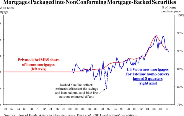
We use updated data from Duca, Johnson, Muellbauer and Murphy (2010) on average loan-to-value (LTV) ratios for first-time home-buyers, the marginal buyers most affected by credit constraints. This series, which spans the period 1979 to 2009, is derived from the American Housing Survey. We argue that the adjusted, first-time buyer LTV series captures exogenous shifts in credit standards. Consistent with a weakening of credit standards during the subprime boom, the LTVs for first-time homebuyers are positively correlated with the share of mortgages outstanding that were securitized into private-label mortgage-backed securities (MBSs, Figure 1). MBSs issued by Fannie Mae and Freddie Mac usually securitized conforming loans, which met credit standards applied to most mortgages in earlier years. In contrast, nonprime mortgages were mainly funded by being packaged into “private label” MBSs because they did not conform to Fannie Mae or Freddie Mac standards, or were too risky to be held by regulated banks (Credit Suisse, 2007). Because our LTV series reflects credit standards on new mortgages (originations), it leads the private MBS share of the stock of home mortgages by about two years. In addition, the rise of the LTV ratio through the mid-2000’s coincided with a large rise in

home-ownership, which was disproportionately concentrated in households under 29 years of age (Bardhan et. al, 2009, pp.7-8). Because such households have limited savings, the timing is consistent with the interpretation that the rise of LTVs for first-time homebuyers in the early 2000’s eased credit constraints for the marginal home-buyer, thereby bolstering the effective demand for housing. This last aspect makes LTV ratios for first-time buyers less prone to endogeneity than house payment-to-income (PTI) ratios. PTI ratios are affected by shifts in interest rates and income, two other components of the inverted demand cointegrating vector, whereas we find that the LTV ratio, adjusted for changes in unemployment, is weakly exogenous in our vector error correction model.

75% 80% 85% 90% 95% 100% -20 -10 0 10 20 30 60 62 64 66 68 70 72 74 76 78 80 82 84 86 88 90 92 94 96 98 00 02 04 06 08 10

Share of Home Mortgage Debt Funded by

percent total debt

Figure 1: LTV Ratios for 1st Time Homebuyers Trends with Share of

Mortgages Packaged into NonConforming Mortgage-Backed Securities

Private-label MBS share of home mortgages

(left axis)

% of all home mortgage

Dashed blue line reflects estimated effects of the savings and loan bailout, solid blue line

nets out estimated effects

% of home purchase price

Sources: Flow of Funds, American Housing Survey, Duca et al., (2011) and authors' calculations.

LTVs on new mortgages for 1st-time home-buyers

lagged 8 quarters (right axis)

The rise in LTV ratios over 2000-05 reflects two types of financial innovation that appeared to enable the risk in nonprime mortgages to be priced and such mortgages to be funded. One was credit scoring technology, which lenders increasingly used to sort and price nonprime mortgages, which had higher LTVs than conventional mortgages (Credit Suisse, 2007). The

second innovation was the development of new structured mortgage products. Partly owing to regulatory concerns, subprime mortgages were not funded by being held in portfolio at banks. Instead, innovations in structured finance enabled such loans to be packaged into collateralized debt obligations (CDOs) or into private-label MBSs that insured investors from mortgage default risk with credit default swaps (CDSs).

During the subprime boom, loans were extended to many borrowers with low down- payments and poor credit histories, who would have earlier been denied loans. Many nonprime loans were adjustable rate mortgages whose initial teaser interest rates benefited from very low Treasury interest rates over 2001–2003. The house-price rises, set in train by these credit-supply and interest-rate changes, enabled nonprime borrowers who faced difficulty paying their mortgages to either pay off their mortgages by selling their homes or to borrow more against appreciated values. However, fundamentals changed from 2003-2004 onwards as interest rates returned to more ‘normal’ levels and high rates of building expanded the housing stock. House prices became increasingly overvalued. With the slowing of the pace of house price appreciation, the extent of bad loans became clearer and with the reassessment of loan quality fundamentals, the supply of credit for all types of mortgages contracted. Specifically, large unexpected loan losses overwhelmed the ability of CDO’s to protect investment-grade tranches from higher

nonprime mortgage defaults (Duca et al., 2010). These losses induced jumps in the cost of using

CDS protection that made subprime mortgage pools too costly to insure. Subprime mortgage funding and originations fell, as reflected by declines in the share of all outstanding mortgages packaged into private-label MBSs (Figure 1). As a result, LTVs for first-time home buyers fell, lowering the effective demand for housing and inducing an unwinding of earlier rises in house prices.

Adding LTV data on first time home-buyers improves house price models in important ways. First, doing so yields more stable long-run relationships, more sensible estimated income

and price elasticities, better speeds of adjustment, and better model fits. Second, this occurs in samples before LTVs rose in the subprime mortgage boom as an earlier, modest rise in LTV ratios enables us to identify such an effect. In another study, we find that adding data on LTVs and regional housing stocks qualitatively improves regional home price models, paralleling the UK regional results of Cameron, Muellbauer and Murphy (2006).

This outline of recent history and these empirical findings are in line with Geanakoplos (2010) who argues that leverage cycles play an important causal role in driving booms and busts of asset prices. The prime measure of leverage for households is the LTV and Geanakoplos gathers data on LTVs for private label subprime and alt-prime mortgages. He shows that, for the upper 50 percent of the distribution of such LTVs, the mean LTV rose strongly from 2000, peaked in 2006Q2 and by 2009 had plunged below levels experienced in 2000. His data do not distinguish first-time buyers and are not representative of the entire private sector mortgage market. But they corroborate the overall picture presented in Figure 1 above.

This study is organized as follows. Section II presents our model of the inverted demand for housing services and section III the data. Models are estimated using cointegration methods in Section IV. Section V simulates recent house prices, accounting for tax credits. The conclusion reviews the empirical results and relates them to recent booms and busts in the U.S. mortgage and housing markets.

II. House Price Models Using the Inverted Demand Approach

Perhaps the simplest theory of what determines house prices is to treat supply—the stock of houses—as given in the short run, with prices driven by the inverted demand for housing services (h) that are proportional to the housing stock (hs). Let log housing demand be given by

where hp = real house price, y = real income and z = other demand shifters including the real user cost of housing, uc and credit constraints, cc.1 2 The own price elasticity of demand is -α and the income elasticity is β. Solving and substituting in for z yields:

(

)

1

lnhp βln – lny hs– lnγ uc– lnδ cc

α

= (2)

Plausible priors for the long run elasticities are the central estimates of time series studies cited in Meen (2001, p. 129) inter alia, implying a price elasticity −α around -0.5 and a long-run income elasticity β around 1.3. As Meen (2001) notes, long-run income elasticity estimates tend to be higher in time series than in cross-section studies owing to transactions and other adjustment costs.

Since housing is a durable good, inter-temporal considerations imply that ‘permanent’ income and ‘user cost’ are important drivers. The user cost takes into account that durable goods deteriorate, but may appreciate in price and incur an interest cost of financing as well as tax. The

usual approximation is that the real user cost is

(

e

)

uc=hp r+ + −δ t hp hp , where r is the real after-tax interest rate of borrowing, possibly adjusted for risk, δ is the depreciation rate, t is the

property tax rate and e

hp hp is the expected real rate of capital appreciation.

Ex-post measures of user costs can be negative if appreciation rates in house price booms exceed nominal user costs. An important issue is how to track expected house price appreciation. Many studies argue that lagged rates of appreciation are good proxy, suggesting a role for extrapolation in the formation of household expectations. We measure real user costs using the lagged annual rate of appreciation over the prior 4 years adjusted for an assumed 8 percent cost

1 _{Inverse demand functions have a long history going back to a 1909 Danish study cited by Theil (1976).} 2

Non-housing wealth was insignificant in our models, likely reflecting that (1) non-housing wealth-to-income ratios may reflect substitution between housing and non-housing wealth offsetting positive wealth effects and (2) the distribution of stock wealth is highly concentrated. Tracy et al. (1999) find that stock wealth was the largest component of net wealth for 5% of households and housing wealth, for 60 percent, with net wealth low among the remaining 35%.

of selling a home. Our user cost measure uc is always positive making lnuc defined over the sample. The log transformation implies that at low values, variations in uc have a more powerful effect than at high values, capturing the notion that household become frenzied that when appreciation is high relative to tax and interest costs.3

Other factors may also be relevant for housing demand, given that many mortgage borrowers face limits on their borrowing and may be risk averse. These could include nominal as well as real interest rates, demography and proxies for risk, particularly of mortgage default. In the dynamics, lagged price adjustment is plausible, given the inefficiency of house prices.4 The rate of change in the per capita housing stock, as well as its level, also likely helps explain house prices. One interpretation is through expectations: households observing much construction might lower expectations of future appreciation. Another interpretation is in terms of prices adjusting both to stock and flow disequilibria, for which error or equilibrium correction models are well suited. We implement this strategy by estimating vector error- correction (VEC) and autoregressive distributed lag (ARDL), versions of the following house price model:

(

)

1 1 0 1 1 2 1 3 1 4 1 1 2 3 4 0 , ln ln ln – ln – ln – ln ln ln ln ln ln + t t t t t t s t s s t s s t s s t s s j s s s t s k k t t s k hp hp y hs uc cc hp y hs uc cc z u α β β β β β γ γ γ γ γ γ δ − − − − − − − − − − ∆ = − − + ∆ + ∆ + ∆ + ∆ + ∆ + +

∑

∑

∑

∑

∑

∑

(3)

with lagged levels and first differences terms, a set of exogenous z variables mainly reflecting

tax, monetary policy and regulatory factors and a random error term u.

3

Hendry (1984) and Muellbauer and Murphy (1997) include similar ‘frenzy’ effects using a cubic in the recent or fitted rate of appreciation. In results not shown, we found that models using lnuc and models linear in uc, but which include a cubic in lagged appreciation, yield similar long run solutions and adjustment speeds.

4

Hamilton and Schwab (1985), Case and Shiller (1989, 1990), Poterba (1991) and Meese and Wallace (1994) find that house price changes are positively correlated and past information on housing fundamentals can forecast future excess returns. Hamilton and Schwab (1985), Capozza and Seguin (1996) and Clayton (1997) find significant evidence against the hypothesis of rational home price expectations. We find that user costs based on the four-year lagged appreciation rate outperformed those based on other lag lengths in LTV and non-LTV models.

III. Data

The variables used fall into the following categories: house prices and the housing stock, permanent income, real user cost of housing, mortgage credit standards, capital gains taxes and monetary/regulatory variables. So far, shifts in demographics variables were insignificant or had counter-intuitive signs in regressions not shown. We plan to further investigate adding demographic effects in future research.

Houses Prices and the Housing Stock. We use Freddie Mac data on nominal house prices from

repeat home sales, t omitting upwardly distorted price appraisals from mortgage refinancings. We seasonally adjust this index before deflating it with the personal consumption expenditures (PCE) deflator to measure real house prices (HP). Because shocks to real energy prices can temporarily distort this deflator, models include the t and t-1 lags of the change in the log of PCE energy prices divided by the non-energy PCE price deflator (∆rpenergy) to clean up residuals from relative energy shocks. The real, per capita housing stock (hs) is the Flow of Funds estimated replacement cost of household sector residential housing structures deflated by the price index for housing construction.

Permanent Income. Our income measure is an estimate of permanent income, since households

tend to abstract from temporary income fluctuations and buy housing and other durable goods based on expected future income. We base the proxy on per capita real non property disposable income. Non property income is the sum of labor and transfer income adjusted for temporary tax effects (see Blinder and Deaton), deflated by the personal consumption expenditures (PCE)

deflator.5 Non-property income (Y) is used because it accords with theory and avoid simultaneity

bias by omitting property income, which reflects property values. Our permanent income

measure p

Y equals the discounted path of expected non-property income over a finite horizon.

5

These include the tax surcharges during the Vietnam War, temporary tax cuts in 1975, 2001, 2005 and 2008; but not Blinder and Deaton’s estimates for the phase-in of the tax cuts of the early 1980s. The details are available upon request. We also net out the impact of the new Medicare part D drug benefit on transfer income since 2006q1.

We estimate equations for the deviation of log ‘permanent’ income from log current income:

(

) (

1

) (

1

)

1 1 ln p K s ln K s ln t t s t t s s t Y Y δ −E Y δ − Y = + =

≈ ∑ ∑ − , a weighted moving average of

forward-looking income growth rates, see Campbell (1997). Permanent income was constructed using a

40 quarter horizon (K=40) and a 10% quarterly discount rate (δ =0.1), consistent with the view

that households view the future with a high degree of uncertainty.

For expectations of the deviation of permanent income from current income, we use a simple model based on reversion to a split trend (with a slow-down in growth from 1968) with just two economic drivers. These are the four-quarter change in the 3 month Treasury bill yield,

3m

TBill , representing the impact of monetary policy, and a Michigan survey measure of consumer expectations (ICE). This has the advantage of being based on a survey of actual consumers.6

The estimated model for

(

1

) (

1

)

1 1 ln perm K s ln K s ln t s t s s t Y δ − Y δ − Y = + = ∆ ≡ ∑ ∑ − is: 68 3 (18.6) (17.4) (13.0) (10.9) (5.6) (6.8) ln perm 0.917 0.533ln 0.0054 0.0033 0.0024 4 m 0.00048 t t t t Y Y t t Tbill ICE ∆ = − + − − ∆ +

with R2=0.87,SE=0.0094and sample period 1961q1 to 2006q4. The variables tand 68

t are a time trend and split time trend respectively. The fitted or forecast (2007q1 onwards) values of

ln perm t

Y

∆ are used to constructln p

t

Y , our measure of permanent income.

Real User Cost of Housing. The real user cost (uc) is the after-tax sum of the effective conventional mortgage interest rate and the property tax rate from the Federal Reserve Board (FRB) model plus the FRB depreciation rate for housing minus the annualized home price appreciation over the four prior years, adjusted for an assumed 8 percent cost of selling a home.

6

The model for permanent income was derived from a more general model including changes in the unemployment rate and the log real S&P 500 index, but these had ‘wrong’ signs or were insignificant.

The resulting real user cost is exceeds zero in the sample, allowing real user costs to enter in

logs, an appealing aspect for reasons stressed by Meen (2001).7

We also adjust the real user cost for the impact of the first-time homebuyer tax credit in 2009. This credit equalled 10% of a home’s sales price, with the credit capped at $8,000 or about 3.3 percent of the average price of existing single-family homes sold in the four quarters (2007q4 to 2008q3) before expectations that the credit would become law. First-time buyers, on average, bought homes that were 20% less expensive than the average price of homes purchased according to the 2005 American Housing Survey. Applying this 20% adjustment implies that the credit equalled about 4.1 percent of the price of homes bought by first-time home-buyers.

The tax credit was passed in the first quarter of 2009 and was extended for sales through June 2010. To model this, we reduced the real user cost of housing 4.11 percentage points for 2008q4 to 2010q2. This basically treats the tax credit as having an effect proportional to its impact on real user costs facing the marginal (i.e. first-time) home buyer. The treatment of the 2008q4 reading reflects the t-1 dating on the level and first first-difference term on real user costs in the model. In other regressions, we found that not adjusting the real user cost in this way led to poorer model fits and slower estimated speeds of adjustments in the LTV and non-LTV models. Mortgage Credit Standards. Mortgage credit standards are tracked by the average LTV for homes bought by first-time home buyers (Duca, Johnson, Muellbauer and Murphy, 2010), based on American Housing Survey data since 1979. This series consistently measures LTV ratios on conventional mortgages, which corresponds to the Freddie Mac house price series that is based on homes bought with conforming conventional mortgages. This LTV series shifted up, from around 85% in the late 1970s and the 1980s to about 87 percent in the 1990s (Figure 1), before jumping after 2002. The rise in the LTV ratio in the early 1990s coincided with Congressional

7

Some autoregressive distributed lag or ARDL models split the user cost term into nominal user cost and appreciation terms to assess issues regarding speculation. However, this approach increases the size, and possibly the number, of the estimated cointegrating vectors when using a vector error-correction (VEC) models.

directives to Fannie Mae and Freddie Mac to increase homeownership by funding more low down-payment mortgages (Gabriel and Rosenthal, 2010).

We adjust raw quarterly AHS LTV data for two reasons. First, we adjust the raw data for seasonality, some unusually small quarterly samples and shifts in regional composition. These latter two factors introduce noise from which we wish to abstract. Second, we examined whether LTVs were endogenous to several macroeconomic variables over 1979-2007, finding no significant link with income and interest rates but a statistical link with changes in the overall unemployment rate (UR). We used the Kalman filter and a local level model with fixed seasonals and a range of explanatory variables, including the change in the civilian

unemployment rate ( civ

UR

∆ ), the share of first time buyers in the West region (West) and dummies for the quarter following the September 11, 2001 terrorist attack ( 9/11

D ) and last two quarters of 1989, corresponding to the Savings and Loan / Thrift bailout ( S&L

D ).

The estimated model is:

_{9/11 &} 9 4 1 1 (3.4) (2.4) (3.0) (3.5) 0.027 civ 0.074 0.060 0.052 S L t t t t t t _j j j _k k k LTV Level UR West D D d D s S = = = − ∆ + − − +

∑

+

∑

withR2 =0.65,SE=0.02,DW =1.84, t stats are in parentheses and the sample period is 1979q1 to

2009q2. The ratio of the estimated variances of the level to the irregular variances is 0.083.

t

Level is the estimated stochastic trend, the Dj's are a series of dummies for small sample

quarters, when credit was tight and the S_k's are fixed seasonal dummies. The positive coefficient

on West plausibly reflects the impact of higher house prices in that region on preferences with respect to LTV ratios, as well as the tendency for faster house price appreciation which may make lenders feel comfortable with smaller down-payment cushions. The dummy variables for quarters with less than 20 observations - 1981q4, 1982q2 to q4, 1983q4, 1993q4, 2005q4, 2007q4 and 2008q4 - were all significant at the 10% level or better. Our adjusted first-time buyer LTV measure consists of the smoothed level and estimated residual from our model. We then

took a three-quarter, weighted average of the resulting series, using quarters t through t-2, where the weights were the relative share of observations in each of the three quarters. This smoothes the series, with the observation weights treating individual borrowers equally.

The 2000 to 2005 rise in LTV ratios likely reflects two financial innovations that fostered the securitized financing of riskier mortgages. The adoption of credit scoring technology enabled lenders to sort nonprime borrowers and attempt to price the risk of nonprime mortgages. Since these loans were too risky for banks to hold, they were funded by securities markets, where investor demand for the mortgage-backed securities funding nonprime loans was temporarily boosted by two unusual developments. The first was the combination of low interest rates and expanded credit availability in the early 2000s fueled a rise in house prices that plausibly led

investors and analysts to under-estimate the default risk on nonprime mortgages. As Duca, et al.

(2010) illustrate, the short history of subprime mortgages over 1998-2006 may have tempted analysts to forecast problem loans on labor market conditions while not having enough sample to disentangle the impacts of house prices and interest rates. In addition, the tendency for vintages of Alt A mortgages to have progressively higher proportions of no- or low-documentation of income (Credit Suisse, 2007) and to post progressively worsening loan quality (Mayer, Pence and Sherlund, 2009) suggests that an errors-in-variables problem from overstatements of borrower income contributed to the underestimation of nonprime mortgage defaults.

The financial innovations that sorted borrowers or funded their loans were accompanied by a second major development - changes in regulations and public policies leading to non-cyclical increases in the demand for the securities funding these mortgages. This included a 2004 SEC decision that doubled the 1935 limits on investment bank leverage from 15:1 to 33:1 and the rise of hedge funds and SIVs that used short-duration debt to fund risky long positions in nonprime mortgages. Also important were large purchases of nonprime MBS by Fannie Mae and Freddie Mac to meet their public policy goals of expanding home ownership (Frame, 2008)

even though they did not issue much nonprime MBS. Technological and policy innovations fostered originations of nonprime mortgages, which were sold to the GSEs or private investors in the form of collateralized debt obligations (CDOs) or with protection from credit default swaps (CDSs). The later failure of CDOs to protect investors from unanticipated defaults and the soaring cost of using CDSs led to a collapse in the funding and availability of nonprime mortgages. As a result, the LTV ratio for first-time buyers fell, partially reversing increases of the early to mid 2000’s.

Capital Gains Taxes. Although income tax rates are in the user cost of capital variable, capital gains tax changes have notably affected house prices. Before mid 1997, net capital gains on home sales were taxable for households under age 55, if the seller did not purchase a home of equal or greater value. The Tax Reform Act of 1997, passed in the second quarter of 1997, largely eliminated this tax by exempting the first $500,000 ($250,000) of gains for married (single) filers, raising the after-tax value of homes and encouraging turnover (Cunningham and Englehardt, 2008). To control for this, we included a variable (CGT) equal to 1 since 1997q4 and 0 before.8 The 1997q4 timing reflects the 1-2 month lag between the signing and actual settlement (when house prices are recorded) of home sale contracts and the t-1 lag on levels variables in the VEC and ARDL models.

Monetary and Regulatory Variables. One variable (MoneyTarget) equals 1 over the money targeting regime of 1979q4 to 1982q3, which likely reduced the supply of or demand for

mortgages by raising interest rate uncertainty. Another is REGQ, Duca’s (1996) measure of how

much Regulation Q ceilings on deposit interest rates were binding until the controls ended. We include the two quarter change, REGQt-1 - REGQt-3, to control for short-run negative short-run disintermediation effects (Jaffee and Rosen, 1979) not consistently tracked by user costs (Duca and Wu, 2009) and to control for a particular aspect of financial liberalization.

8

Another variable controls for an large rise in the upfront insurance premium for Federal Housing Administration (FHA) loans which provide government guarantees against losses to lenders.9 A rise in the upfront premium (from 0 to 3.8% of the mortgage principal) was announced to take effect in late 1983q3, inducing many renters to leave rental housing and purchase “starter” homes in that quarter. This hike was later partially reduced by smaller premium cuts that were too small to be significant. We include a dummy equal to 1 in 1983q3

and 0 otherwise (∆FHAFee) to control for the large, induced jump in house prices that quarter.

IV. Econometric Results

In this Section, we present our cointegrating model results. The data have unit roots so we estimate vector error correction (VEC) models, as well as simpler autoregressive distributed lag (ARDL) models. The VEC models are estimated in two stages. In the first stage, the long-run cointegrating regressions are estimated using the Johansen (1991, 1995) method. The second stage is akin to second step of the Engle-Granger (1987) procedure.

In both types of models, we control for a variety of tax effects - beyond using income and property tax rates in calculating the user cost of housing- and for the money targeting regime of 1979-1982 that imparted more interest rate risk to house prices beyond that reflected in simple user cost of capital variables. By addressing such factors, we try to avoid omitted variable bias that can obscure long-term, qualitative relationships and lead to poorly estimated coefficients.

The VEC results in the upper panel of Table 1 set out the long-run, unique cointegrating relationship, corresponding to equation (2), between house prices, permanent income, the real user cost of housing, the housing stock and our credit proxy, the adjusted LTV ratio for first time

9

buyers. Columns 1 and 2 exclude the latter variable, whereas columns 3 and 4 include it.10. Each model includes the monetary targeting, Regulation Q, FHA fees and capital gains tax regime controls as exogenous variables. Our models are estimated over two samples. Models 2 and 5 are estimated over the complete sample 1981q2 to 2009q3. Models 1 and 4 were estimated over a shorter sample ending in 2002q2, just after the large temporary swings in income and other variables from the September 11 terror attacks and just before LTV ratios rose during the subprime boom starting in 2002. The lag lengths of the VEC models were chosen to generate (at most) a unique, significant cointegrating vector and clean residuals where possible.

Although cointegrating vectors with the expected signs are found for both the non-LTV and LTV models, the latter are better in several ways. First, the LTV variable is correctly signed and highly significant, consistent with our view that the adjusted, first time buyer LTV ratio is proxying credit constraints and the house price-to-rent model results in Duca et al. (2011). Second, there is stronger evidence of cointegration in the full sample from the maximal eigenvalue statistics when the LTV ratio is included. In addition, the long-run housing stock variable is more significant in the full sample LTV model versus the non-LTV model. Third, including LTV ratios yields more plausible elasticities, especially in the full sample. The inverse of the coefficient on log housing stock, interpretable as the long run price elasticity of demand, is between -0.48 to -0.57, which is smack in the middle of the range of cross-section and time series estimates reported in Meen (2001). Contrast these with the price elasticity estimates of -0.58 and -0.76 in the non-LTV models. Furthermore, the implied income elasticity of housing demand – the ratio of the estimated, long run coefficients on log income and log housing stock – range between 1.35 and 1.36 in the LTV models and 1.53 to 1.57 in the non-LTV models. The former are closer to the time series estimates reported in the literature.

10

In the long run cointegratimg regressions, the log LTV ratio enters with a one period lag. This lag improved model fit, perhaps reflecting a time delay before first-time homebuyers learn of changes in less visible down-payment constraints.

Another advantage of the LTV models vis-à-vis the non-LTV models is that the implied equilibrium levels of real house prices line up somewhat better with actual real house prices. This can be seen from equilibrium values constructed from coefficients estimated over the shorter sample period ending in 2002q2 to 2009q3, as shown in Figure 2. Here the four-quarter lag of equilibrium log levels from the LTV models more closely line up with actual real house prices, when LTVs fell during the credit crunch period of the early 1990s and when LTVs surged during the subprime boom of 2003 to 2006.

LTV models also outperform non-LTV models in their ability to track short-term changes

in real house prices (lower panel, Table 1). In short-run models, the monetary regime, REGQ,

and capital gains variables are significant with expected signs, while the FHA variable is marginally significant in the models, except in the full sample non-LTV model. The coefficients on lagged changes in the per capita housing stocks tend to be negative, as expected, and in line with UK results (Cameron et al., 2006). The income dynamics are consistent with a moving average of income. The dynamics in log real user cost also imply a moving average. Short run dynamics in lagged house price changes suggest a positive short term momentum effect, aside from that embedded in the real user cost term.

The LTV models fit somewhat better – their adjusted R2’s are .01 to .03 higher and standard errors are 5 to 14 percent smaller than in the corresponding non-LTV models. In the full sample the LTV model (model 4) has an estimated 11.3% speed of adjustment, which is much more plausible than the 5.4% speed in the corresponding non-LTV model (model 2). Moreover, the speed of adjustment is stable across the two samples for the LTV models, but not for the non-LTV models where the speed of adjustment falls from 15.7% to 5.4%. A plausible interpretation of the better long and short-run performance of the LTV models is that non-LTV models omit information about credit standards, which were an important driver, along with real interest rates, of the recent boom and bust in U.S. house prices.

4.8 4.9 5 5.1 5.2 5.3 5.4 5.5 5.6 5.7 5.8 '82 '83 '84 '85 '86 '87 '88 '89 '90 '91 '92 '93 '94 '95 '96 '97 '98 '99 '00 '01 '02 '03 '04 '05 06 07 08 09 ln equilibrium nonLTV model 1 4-quarter lag est. 1981q3-2002q2 equilibrium LTV model 4 4-quarter lag est. 1981q3 -2002q2 actual real house prices

Figure 2: Pressures on Real House Prices During Boom and Bust Better Tracked by Out-of-Sample Equilibrium Values From the LTV Model

1st-time homebuyer tax credit lowers real

user costs, pushing up equilibrium prices until 2010:q2

Autoregressive Distributed Lag Models. As a check, we estimated ARDL models over the full

sample, with and without our LTV variables.11 Although the VECM results are generally

preferable, it is reassuring that the estimated long-run elasticities of housing demand and speeds of adjustment (the coefficient on lagged real house prices) in the two ARDL are similar to those from their VEC counterparts. For brevity, we show only the ARDL LTV model results in column 5. The non-LTV ARDL results are available upon request.

Exogeneity. A natural question is whether the LTV series is endogenous. If the LTV series were driven by house prices, this would greatly complicate and alter the interpretation of our findings. In the full sample, complete VEC system underlying the Column (4) results, the house price error correction term is insignificant (t statistic of -0.99) in the LTV equation, indicating that the LTV ratio is weakly exogenous to the other variables, as is the case for the real user cost (tstatistic of 0.89), permanent income (t(tstatistic of 1.34) and the housing stock (t(tstatistic of

11

The specification of the ARDL models is slightly different from that of the ARDL models. In particular, a more parsimonious set of lagged first difference terms are used. Further details are available on request.

1.47). Thus, consistent with theory, equilibrium house prices are indeed driven by shifting credit standards as well as changes in income, user costs and the housing stock.

The 2009 First Time Buyer Tax Credit. In order to gauge the effect of the tax credit, we estimated the LTV model in columns 4 and 5 of Table 1 up to 2008q4, the period before the tax credit appears in the lagged real user cost terms. We then dynamically simulated the model with and without the tax credit. The simulation results suggest that the tax credit had a significant positive effect on the level and time path of house prices – house prices might have fallen (undershot) by as much as 10% more by the end of 2010, and stayed lower for longer, without the temporary tax credit. The results reflect the ‘bubble builder’ and ‘bubble burster’ features of our error correction house price model (Abraham and Hendershott, 1996).

Results Using the Loan Performance Measure of House Prices. As a robustness check, we also

estimated inverted demand models using a median single family house price series from Loan Performance, covering all securitized mortgages - including more subprime and other nonprime mortgages than the Freddie Mac series.12 The Loan Performance (LP) data cover a slightly shorter sample (we lose 1981) and display more pronounced and somewhat faster swings in

house prices albeit similar long-run trends.13 The LP data imply faster house price appreciation

resulting in negative real user costs in the mid-2000s. This means that we have to use the level, rather than the log, of the user cost to model the LP house price series.

The tendency for the Loan Performance house prices series to move more quickly than the Freddie Mac series reflects the fact that the LP series includes more thinly traded low-end homes (financed with nonconforming subprime and FHA loans) and high-end homes (financed with jumbo and alternative A loans). Likely reflecting this timing difference, we found that only the time t change in relative energy prices was significant. Because the FHA and capital gains

12

This series excludes the prices of repossessed homes or homes sold in short-sales, because the sellers of such homes have very different incentives and time horizons from those of owner-occupiers.

13

tax dummies were insignificant, we dropped them. To handle a large positive outlier in 2009q2

we added a dummy (TaxCredit) for this quarter. This variableis significant in both the non-LTV

and LTV LP models (columns 6 and 7 of Table 1), with coefficients suggesting a ceteris paribis

4½ to 5 percentage point jump in prices, consistent with the passage of the tax credit legislation in 2009q2, with retrospective provisions for 2009q1.

It is very reassuring that, using the Loan Performance house price data, the LTV ratio is highly significant and exogenous to our VEC system (Column 7, Table 1), the same as in the LTV models using Freddie Mac data (Columns 3 to 5). As before, including the LTV ratio yields a unique cointegrating vector, improves model fit and results in a much faster quarterly speed of adjustment (9.0%) than in its non-LTV counterpart (3.4%, column 6). The implied long-run income elasticity is also similar to the estimates based on the Freddie Mac house price series, although the estimates should be interpreted carefully since the user cost terms are not logged. The LP data are more volatile than the Freddie Mac data, so it is not surprising that the

fit of the LP models is poorer. For example, the adjusted R2 in column 7 is 8 percentage point

lower than in column 5, whilst the equation standard error is twice as large.

V. Where Are House Prices Heading?

To shed light on how much U.S. house prices may be overvalued, we now examine the implications of our house price models for the deviations of prices from their ‘equilibrium’ or ‘long-run’ values. There is more than one concept of equilibrium. The narrow concept is conditional on the observed log real user cost as used in our econometric models. Consider the

VEC results in Column (4) of Table 1. The long run solution is lnhp = 4.71 -0.21lnuc + 2.80lnyp

– 2.07lnhs + 0.97lnLTV. Conditional on lnuc, the deviation from equilibrium is lnhp – (4.71 -0.21lnuc + 2.80lnyp– 2.07lnhs + 0.97lnLTV). Using such measures, real house prices were over-valued in 2009q3 by about 10% in both the LTV (column 5) and non-LTV (column 2) models.

An advantage of LTV models is their better ability to pin down long-run house prices as implied by the partly dynamic, out-of-sample forecasts generated using the short sample (1981q2 to 2002q2) models. The forecasts are partly dynamic since we assume that house prices at time t-2 are known and house prices at time t -1 are the model forecasts from last period. This dating structure is consistent with the reporting lags in the Freddie Mac house price series that we use. As shown in Figure 3, near the height of the house price boom, the LTV and non-LTV models have similar, reasonably-sized misses, with the former tending to over-predict and the latter to under-predict house prices in the mid-2000s. However, since late 2008 the LTV model tracks actual house prices more closely, while the non-LTV model is persistently off. This is especially true if one assumes that LTVs stabilized near their 2009q2 levels and one extends the forecast to 2010q2, the latest period for which we have actual house price data.

Another way to assess possible overvaluation is to forecast house prices out-of-sample (post 2009q3) using the full sample estimates in Columns (2) and (4) of Table 1. In order to do this, we have to specify reasonable values for future income, the housing stock, interest rates, loan to value ratios, etc... We assume that LTVs remain at 2009q2 levels. Actual non-LTV data are used through 2010q2. Non-property income is assumed to grow in line with average personal income growth forecasts from the October and November 2010 Blue Chip Economic Indicators survey of forecasters. We based a path for the real housing stock off private sector projections that total housing starts would return to a long-run equilibrium pace of 1.4 million units in early 2012, up from the current 0.6 million units.14 We assume that the tax credit for home-buyers expired in 2010q2 for good, but keep depreciation and other tax variables at their 2010q2 levels. These assumptions are combined with average forecasts of mortgage interest

14 _{We assume starts are at a 0.6 million unit annual pace through 2010q4, and then rise 0.05 million per quarter until}

reaching 1.4 million units in 2014q4. From this pace, we construct a shortfall of starts from their long-run pace (1.4 million units), which averaged 0.8 million per quarter over 2008q3 to 2010q2. Lagging one quarter for time to build lags, the real per capita housing stock fell by 0.23845 percent per quarter from 2008q4 to 2010q2, or by 0.23845/.8 percent per 0.1 million shortfall in housing starts. Using this ratio and projected shortfalls in housing starts, the real per capita housing stock falls until 2013q1 and we assume it rises in line with per capita real income thereafter.

rates from the December 2010 Blue Chip Financial Forecasts to construct a nominal user cost path. 5.1 5.2 5.3 5.4 5.5 5.6 5.7 '02 '03 '04 '05 06 07 08 09 10

Figure 3: LTV Model Outperforms nonLTV Model in Tracking the Log-Level of Real House Prices Out-of-Sample

Actual LTV Model Forecasts Non-LTV Model Forecasts ln period of home-buyer tax credit

We use one-quarter lagged forecasts of house prices to construct the appreciation series used to convert the nominal into a real user cost series. Because an error-correction model is used, with lagged house price change and real user cost terms, where the latter are constructed using the annualized changes in house prices over the prior four years, the model captures the ‘bubble builder’ and ‘bubble burster’ dynamics emphasised by Abraham and Hendershott (1996), inter alia.

Using the assumptions set out above, the dynamic simulations from the LTV model imply that nominal house prices may fall 8 percent further from their simulated 2010q2 levels

before hitting bottom in 2011q4 (Figure 4), with real prices falling 10 percent by 2012q1.15 The

declines are less dramatic in the non-LTV models - nominal house prices only fall 6 percent

15

This result is not far from the simulated 5 percent decline in nominal house prices that we discussed in an early draft of our related house price-to-rent paper (Duca et al., 2011).

below their simulated 20102q levels in 2011q4, whilst real house prices bottom out 8 percent below their simulated 2010q2 levels. In the three quarters following 2009q3 for which we have actual house price data, the LTV and non-LTV model simulations straddle actual prices, with the LTV model tracking a little better. Partial data for 2010q3 suggest a notable decline in nominal house prices that is closer to the level generated by the LTV model. In the simulations, the nominal level of the Freddie Mac house price series only reverts to its 2007q2 subprime boom peak in late 2014 / early 2015.

4.8 5 5.2 5.4 5.6 5.8 6 '95 '96 '97 '98 '99 '00 '01 '02 '03 '04 '05 06 07 08 09 10 11 12 13 14 15

Figure 4: Before Bottoming Out in Late 2011, Nominal House Prices Fall 8 Percent in the LTV Model But Only 6 Percent in the Non-LTV Model

Actual LTV Model Forecasts Non-LTV Model Forecasts ln In-sample Out-of-sample

The simulations, of course, are based on projections of house price determinants which

are hard to predict. One source of such uncertainty stems from changes in public policy. Inter

alia, changes in foreclosure policies could affect the speed at which house prices adjust. Another source stems from changes in federal mortgage programs. Before 2008, FHA mortgage size limits were lower than those on conventional mortgages securitized by Freddie Mac and Fannie Mae. In the spring of 2008, when jumbo and conventional mortgage issuance dried up as jumbo

lenders and the GSE’s tightened credit standards, the FHA increased the maximum size of the loans it guarantees against default risk to the limits used by Freddie Mac and Fannie Mae in most mortgage markets and up to $729,750 in high-priced markets. This effect may not be captured by our LTV measure which omits FHA mortgages (since the number of first time buyers with FHA mortgages in the AHS was very small). In addition, the FHA’s share of mortgage originations rose from 15 percent or so before 2008 to about 50 percent by late 2008.

To explore the possible impact of these effects, we adjusted our LTV series upwards in two ways. The first is to add to our series the increase in the difference between the average overall LTV ratio and the average LTV ratio on private (non-FHA, non-Veterans Administration) mortgages for first-time buyers after 2008q2. This amounted to about ¾ of one

percentage point, which was added to our LTV ratio starting in 2008q2 to create LTVFHA1. The

second is a calculation of a weighted FHA and private mortgage LTV ratio. For this we assume that the minimum down-payment on FHA mortgages is 3½%, to which we add a 2% upfront insurance premium, implying an effective 5.5% minimum down-payment or 94.5% LTV ratio. The 35 percentage point increase in the FHA shares of mortgages implies that, at the end of 2008, FHA mortgages constituted about 41.2 percent of the formerly conventional and jumbo

first time buyer mortgages. Our weighted average LTV, LTVFHA2, was calculated by applying

the 94.5% effective LTV ratio on FHA mortgages to the 41.2% share and the observed average LTV ratio on private mortgages to the remaining 58.8% share. The simulated time path of house prices is similar to that shown in Figure 4, except that real house prices fall by about 1% less

using LTVFHA1 and by about 2½% less using LTVFHA2.

We believe that the simulation results are reasonably robust to alternative formulations of house prices and to endogenizing housing supply, but we have not yet completed our analysis of these issues. For these reasons, the simulation results should be treated with caution.

VI. Conclusion

In the inverted demand approach, credit standards for first-time home-buyers are important determinants of house prices, along with income, real user costs and the housing stock. Our findings indicate that swings in credit standards played a major, if not the major, role in driving the boom and bust of real U.S. house prices in the first decade of this century. Long-term movements in mortgage credit standards for the marginal home-buyer have not generally been tracked and incorporated in standard time series models of U.S. house prices. Consequently, such models are mis-specified and may not track house prices well during periods of shifting credit standards. In contrast, models including a cyclically adjusted LTV measure for first time home-buyers have much better short- and long-run properties. These range from faster speeds of adjustment to better model fits and more sensible and plausible long-run elasticities of housing demand. Overall, our findings fit with the view that many asset bubbles are fueled by unsustainable increases in the availability of credit or in the use of non-robust financial practices.

References

Abraham, Jesse M. and Patric H. Hendershott, (1996), “Bubbles in Metropolitan Housing

Markets”, Journal of Housing Research, 7, 191–207.

Bardhan, Ashok D., Robert E. Edelstein and Cynthia A. Kroll (2009), “The Housing Problem and the Economic Crisis: A Review and Evaluation of Policy Prescriptions,” Fisher Center Working Paper, University of California at Berkeley.

Blinder, Alan and Angus Deaton (1985), “The Time Series Consumption Function Revisited,” Brookings Papers on Economic Activity, 1985(2), 465-511.

Cameron, Gavin, John Muellbauer and Anthony Murphy (2006), “Was There a British House

Price Bubble? Evidence from a Regional Panel”,CEPR discussion paper no. 5619.

Capozza, Dennis and Paul Seguin (1996), “Expectations, Efficiency and Euphoria in the Housing

Market”, Regional Science and Urban Economics 26, 369-86.

Case, Karl E. and Robert J. Shiller (1989), “The Efficiency of the Market for Single-Family

Homes”, American Economic Review 79, 125-37.

Case, Karl E. and Robert J. Shiller (1990), “Forecasting Prices and Excess Returns in the

Housing Market”, Journal of the American Real Estate and Urban Economics

Association, 18, 253-73.

Clayton, Jim (1997), “Are Housing Price Cycles Driven by Irrational Expectations?”, Journal of

Real Estate Finance and Economics 14, 341-63.

Credit Suisse (2007), “Mortgage Quality Du Jour: Underestimated No More”, March 13, 2007. Cunningham, Christopher R. and Gary V. Englehardt (2008), “Housing Capital-Gains Taxation

and Homeowner Mobility: Evidence from the Taxpayer Relief Act of 1997”, Journal of

Urban Economics, 63(3) 803-15.

Davis, Morris A. and Jonathan Heathcote (2005), “The Price and Quantity of Residential Land in

the United States”, International Economic Review, 46, 751-84.

DiMartino, Danielle and Duca, John V. (2007), “The Rise and Fall of Subprime Mortgages”,

Federal Reserve Bank of Dallas Economic Letter, November.

Doms, Mark and John Krainer (2007), “Innovations in Mortgage Markets and Increased Spending on Housing”, Federal Reserve Bank of San Francisco working paper no. 05.

Duca, John V. (1996), “Deposit Deregulation and the Sensitivity of Housing”, Journal of

Duca, John V. (2006), “Making Sense of the U.S. Housing Slowdown”, Federal Reserve Bank of

Dallas Economic Letter, November.

Duca, John V., Kurt B. Johnson, John Muellbauer and Anthony Murphy (2010), “Time Series Estimates of U.S. Mortgage Constraints and Regional Home Supply”, mimeo, Federal Reserve Bank of Dallas.

Duca, John V., John Muellbauer and Anthony Murphy (2009), “The Financial Crisis and Consumption”, mimeo, Federal Reserve Bank of Dallas.

Duca, John V., John Muellbauer and Anthony Murphy (2010), “Housing Markets and the

Financial Crisis of 2007-2009: Lessons for the Future”, Journal of Financial Stability 6,

203-17.

Duca, John V., John Muellbauer and Anthony Murphy (2011), “House Prices and Credit

Constraints: Making Sense of the U.S. Experience”, The Economic Journal, forthcoming.

Duca, John V. and Tao Wu (2009), “Regulation and the Neo-Wicksellian Approach to Monetary

Policy”, Journal of Money, Credit and Banking, 41(3), 799-807.

Engle, Robert F. and Clive W. J. Granger (1987), “Cointegration and Error Correction:

Representation, Estimation and Testing”, Econometrica, 55, 251–76.

Frame, W. Scott (2008), “The 2008 Federal Intervention to Stabilize Fannie Mae and Freddie

Mac,” Journal of Applied Finance, 18(2), 124-36.

Gallin, Joshua (2006), “The Long-Run Relationship between Home Prices and Income: Evidence

from Local Housing Markets”, Real Estate Economics, 34(3), 417-38.

Gabriel, Stuart A. and Stuart S. Rosenthal (2010), “Do the GSE’s Expand the Supply of Mortgage Credit? New Evidence of Crowd Out in the Secondary Mortgage Market”, mimeo, 2010 AEA Annual Conference presentation.

Geanakoplos, John (2010), “Solving the Present Crisis and Managing the Leverage Cycle”, New

York Federal Reserve Economic Policy Review, 16(1), 101-31.

Hamilton, Bruce and Robert Schwab (1985), “Expected Appreciation in Urban Housing

Markets”, Journal of Urban Economics, 18, 103-18.

Hendry, David F. (1984). “Econometric modelling of house prices in the United Kingdom”, in

David F. Hendry and Kenneth F. Wallis (eds), Econometrics and Quantitative

Economics. Oxford: Basil Blackwell.

Himmelberg, Charles, Chris Mayer and Todd Sinai (2005), “Assessing High House Prices:

Bubbles, Fundamentals and Misperceptions”, Journal of Economic Perspectives 19,

Jaffee, Dwight M. and Ken Rosen (1979), “Mortgage Credit Availability and Residential

Construction Activity”, Brookings Papers on Economic Activity, 2, 333-86.

Johansen, Soren (1991), “Estimation and Hypothesis Testing of Cointegration Vectors in

Gaussian Vector Autoregressive Models”, Econometrica, 59, 1551–80.

Johansen, Soren (1995), Likelihood-based Inference in Cointegrated Vector Autoregressive

Models, Oxford: Oxford University Press.

Mayer, Christopher, Karen Pence and Shane M. Sherlund (2009), “The Rise in Mortgage

Defaults”, Journal of Economic Perspectives, 23, Winter, 27-50.

Meen, Geoffrey (2001), Modeling Spatial Housing Markets: Theory, Analysis and Policy,

Norwell, MA: Kluwer Academic Publishers.

Meese, Richard and Nancy Wallace (1994), “Testing the Present Value Relation for Housing

Prices: Should I Leave My House in San Francisco?”, Journal of Urban Economics, 35,

245-66.

Muellbauer, John and Anthony Murphy (1997), “Booms and Busts in the U.K. Housing Market”,

The Economic Journal, 107, 1701–27

Poterba, James (1991), “House Price Dynamics: the Role of Tax Policy and Demography”, Brookings Papers on Economic Activity, 2, 143-203.

Smith, Margaret Huang and Gary Smith (2006), “Bubble, Bubble, Where’s the Housing

Bubble?”, Brookings Papers on Economic Activity, 37, 1-68.

Theil, Henri, (1976), Theory and Measurement of Consumer Demand, Studies in Mathematical

and Managerial Economics, Vol. 21, Amsterdam: North-Holland.

Tracy, Joseph, Henry Schneider and Sewin Chan (1999), “Are Stocks Overtaking Real Estate in

Household Portfolios?”, Federal Reserve Bank of New York Current Issues in

Table 1: Vector Error Correction and Autoregressive Distributed Lag Models of the Change in Real U.S. Log House Prices,∆lnhp

Maximum likelihood systems estimates of the long-run equilibrium relationship ln _{0 1}ln p+ ₂ln

t t t

hp =β +β y β hs +

3lnuct 4lnLTVt 1 ut

β +β − + ,using a 4 (no LTV terms) or 5 (with LTV terms) equation system with at most one

cointegrating vector, apart from the normalized ARDL results in column (5).

Data Freddie Mac Freddie Mac Loan Performance (LP)

LTV Terms No LTV Terms With LTV Terms No LTV LTV

Type of Model VEC VEC VEC VEC ARDL VEC VEC

Sample 81q2- 02q2 81q2-09q3 81q2-02q2 81q2-09q3 81q2-09q3 82q1-09q3 82q1-09q3 (1) (2) (3) (4) (5) (6) (7) Constant 3.792 4.143 4.893 4.711 - 0.790 4.304 lnuct-1 /uct-1 (LP) -0.198** -0.248** -0.240** -0.211** -0.210** -0.005 -0.023** (12.39) (14.21) (14.53) (23.43) (5.02) (0.52) (5.83) 1 ln p t y− 2.627** 2.064** 2.378** 2.796** 2.571** 5.950** 3.508** (6.38) (3.12) (4.61) (7.92) (3.44) (2.16) (3.48) lnhst-1 -1.715** -1.314* -1.747** -2.071** -1.859** -3.896** -2.679** (5.04) (2.31) (3.99) (6.69) (3.10) (2.14) (3.48) lnLTVt-2 - - 1.189** 0.967** 0.712** - 2.893** (4.78) (5.45) (2.44) (4.77) Elasticities:- Income 1.53 1.57 1.36 1.35 1.38 1.53 1.31 Price -0.58 -0.76 -0.57 -0.48 -0.54 -0.26 -0.37 Trace Stats: 1 Vector 70.83** 58.28** 98.56** 101.08** - 54.60** 83.04** 2 Vectors 24.41 27.16 46.99 47.46 - 20.00 41.22 λ _{Max Stats:} 1 Vector 46.42** 31.12* 51.57** 53.62** - 34.59** 41.82** 2 Vectors 19.73 16.11 25.97 22.74 - 12.30 22.53

OLS estimates of the speed of adjustment and short-run dynamics etc. using the estimated equilibrium correction terms

in the upper pane, e.g. ln 0 1ln - 2ln 3ln

p

t t t t t

EC = hp −β −β y β hs −β uc −β4lnLTVt−1.

Data Freddie Mac Freddie Mac Loan Performance (LP)

LTV Terms No LTV Terms With LTV Terms No LTV LTV

Type of Model VEC VEC VEC VEC ARDL VEC VEC

Sample 81q2- 02q2 81q2-09q3 81q2-02q2 81q2-09q3 81q2-09q3 82q1-09q3 82q1-09q3 (1) (2) (3) (4) (5) (6) (7) Constant 0.001 -0.002 0.003 0.002 0.486** 0.000 0.001 (0.48) (1.40) (1.43) (1.10) (5.00) (0.00) (0.21) ECt-1 -0.157** -0.054** -0.122** -0.113** - -0.034** -0.090** (3.58) (3.25) (5.00) (5.21) (4.26) (5.07) lnhpt-1 - - - - -0.106** - - (5.09) MoneyTargett -0.005 -0.006+ -0.017** -0.011** -0.012** -0.009 -0.022** (1.29) (1.90) (4.13) (3.57) (3.46) (1.546) (3.22) CGTt-2 -0.001 0.001+ 0.002* 0.003** 0.004** - - (0.67) (1.80) (2.16) (4.28) (2.46) ∆2REGQt-1 -0.003 -0.005** -0.004** -0.002* -0.006** - - (1.44) (3.72) (2.94) (2.15) (4.35) ∆_{FHAFeet 0.001 0.004 0.004}+ _0.004+ _0.006* _{- -} (0.37) (1.48) (1.94) (1.67) (2.27) Continued Overleaf