PLEASE CITE THE PUBLISHED VERSION. PUBLISHER

(1)

This item was submitted to Loughborough's Research Repository by the author.

Real-time optimal energy management of electrified engines

PLEASE CITE THE PUBLISHED VERSION

http://dx.doi.org/10.1016/j.ifacol.2016.08.038

PUBLISHER

VERSION

AM (Accepted Manuscript)

PUBLISHER STATEMENT

This work is made available according to the conditions of the Creative Commons Attribution-NonCommercial-NoDerivatives 4.0 International (CC BY-NC-ND 4.0) licence. Full details of this licence are available at:

https://creativecommons.org/licenses/by-nc-nd/4.0/

LICENCE

CC BY-NC-ND 4.0

REPOSITORY RECORD

Zhao, Dezong, Edward Winward, Zhijia Yang, Richard Stobart, and Thomas Steffen. 2017. “Real-time Optimal Energy Management of Electrified Engines”. figshare. https://hdl.handle.net/2134/24483.

(2)

Real-Time Optimal Energy Management of

Electrified Engines

Dezong Zhao∗ Edward Winward∗∗ Zhijia Yang∗

Richard Stobart∗ _{Thomas Steffen}∗

∗_{Department of Aeronautical and Automotive Engineering,}

Loughborough University, Loughborough, UK (e-mail: [email protected], [email protected], [email protected],

[email protected])

∗∗_{Energy & Transportation Research, Caterpillar Inc., Peterborough,}

UK

Abstract: The electrification of engine components offers significant opportunities for fuel

economy improvements, including the use of an electrified turbocharger for engine downsizing and exhaust gas energy recovery. By installing an electrical device on the turbocharger, the excess energy in the air system can be captured, stored, and re-used. This new configuration requires a new control structure to manage the air path dynamics. The selection of optimal setpoints for each operating point is crucial for achieving the full fuel economy benefits. In this paper, a control-oriented model for an electrified turbocharged diesel engine is analysed. Based on this model, a structured approach for selecting control variables is proposed. A model-based multi-input multi-output decoupling controller is designed as the low level controller to track the desired values and to manage internal coupling. An equivalent consumption minimization strategy is employed as the supervisory level controller for real-time energy management. The supervisory level controller and low level controller work together in a cascade which addresses both fuel economy optimization and battery state-of-charge maintenance. The proposed control strategy has been successfully validated on a detailed physical simulation model.

Keywords:electrified engines, fuel economy optimization, real-time energy management, decoupling control, dynamics analysis

1. INTRODUCTION

Motivated by the increasing fuel costs and environmen-tal pressures, countries around the world are passing in-creasingly stricter legislations on the fuel efficiency of internal combustion engines. Heavy duty vehicles (HDVs) contribute almost a quarter of the fuel consumption in transportation, and most are equipped with diesel engines due to their higher thermal efficiency and good durability. With state-of-the-art technologies, an estimated improve-ment in fuel economy of 35% - 50% of HDVs is considered realistic, with most of the potential concentrated on engine efficiency improvement and engine hybridization Boyd and Vandenberghe (2010). The electrified turbocharger is a critical technology in engine hybridization. It combines a variable geometry turbocharger (VGT) and an electric machine (EM) within a single housing. The EM is capable in bi-directional power transfer, so excess power can be recuperated by the EM to supply electrical accessories or to be stored in a battery for later usage. On the other hand, the EM accelerates the turbocharger to improve engine response, especially for transient torque demands. Due to its location in the air system, reasonably small electric systems can have a large effect on transient behavior and engine efficiency. In this sense the technology is superior to conventional hybrid systems that act on the engine crankshaft.

The electrified turbocharger has attracted considerable development interest. The mainstream diesel engine and turbocharger manufacturers have developed their own pro-totype electrified turbochargers, see Bailey (2000), Arnold et al. (2005), and Ibaraki et al. (2006). Investigations into the efficiency characterization of an electrified tur-bocharger through experiments with a heavy duty diesel engine have been made by Terdich and Martinez-Botas (2013) and Terdich et al. (2014). There is a broad agree-ment that the developagree-ment of a systematic strategy in both real-time energy management and input multi-output (MIMO) control is essential for exploring the max-imum benefits of the electrified turbocharger.

A suitable control and energy management structure for the electrified turbocharged diesel engine (ETDE) is still to be established. In Ibaraki et al. (2006), the EM is con-trolled in an open loop manner. In Glenn et al. (2010), the EM, VGT, and exhaust gas recirculation (EGR) valve are controlled independently without considering the internal couplings in the engine or the generation setpoints. In 2014, a consortium led by Caterpillar Inc. developed a cutting-edge electrified turbocharger called electric turbo assist (ETA). Based on the ETA, several control methods and testing systems were developed in Loughborough Uni-versity in simulations Zhao et al. (2015); Zhao and Stobart (2015); Zhao et al. (2016) and experiments Zhao et al. (2014, 2013); Winward et al. (2016); Yang et al. (2016).

(3)

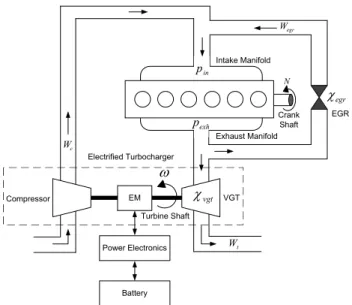
VGT Intake Manifold Exhaust Manifold Compressor EGR  N c W egr W t W Turbine Shaft Crank Shaft in p exh p EM Power Electronics Battery Electrified Turbocharger vgt  egr 

Fig. 1. Electrified turbocharged diesel engine

This paper presents an attempt to address this gap. The main contributions are:

(1) An explicit principle for the selection of control vari-ables of an ETDE is proposed based on the dynamics analysis. From this, clear guideline for the generation of setpoints follow.

(2) A two-level structure of energy flow management and air path regulation is presented. On the supervisory level, the optimal setpoints of control variables are computed to distribute energy flows in the optimal way. On the low level, a MIMO controller is designed to implement the optimal energy flow distribution. (3) An equivalent consumption minimization strategy

(ECMS) algorithm is designed as the supervisory level controller to guarantee the real-time optimization of fuel economy while keeping the sustainable battery usage.

(4) A model-based non-smooth robust controller is de-signed as the low level controller to regulate the air path dynamics and to address the internal couplings among actuators.

(5) The proposed control strategy is successfully applied on a physical engine model for validation.

The paper is organized as follows. Following the intro-duction in section 1, the electrified turbocharger model is described in section 2. The control problem is formulated in section 3, and the control-oriented dynamic system is analyzed in section 4. The supervisory level controller design is presented in section 5, and the low level controller in section 6. Validation results of the strategy are demon-strated in section 7, followed by conclusions in section 8.

2. ELECTRIFIED TURBOCHARGER MODEL The structure of an ETDE is illustrated in Fig. 1, while its variables and related parameters are defined in Table 1. A switched reluctance motor (SRM) is selected as the EM. It is an excellent option in extra-high speed applications thanks to its simple structure, see Bilgin et al. (2015). The EM can work in both assisting (motoring) mode and harvesting (generating) mode. In assisting mode, the EM

Table 1. Nomenclature

Variable Description Unit

N Engine speed rpm

TL Engine load Nm

Wf Engine fuelling rate kg/s Wc Compressor air mass flow rate kg/s Wegr EGR mass flow rate kg/s Wt Turbine gas mass flow rate kg/s F1 Burnt gas fraction, defined as _WWegr

c+Wegr –

λ In-cylinder air-fuel ratio, defined as Wc

Wf –

Pc Compressor power kW

Pt Turbine power kW

Pem EM power kW

pin Intake manifold pressure kPa pexh Exhaust manifold pressure kPa pam Ambient pressure kPa Ta Ambient temperature K

ω Turbine speed rpm

τ Turbocharger time constant s

ηc Compressor isentropic efficiency – ηt Turbine isentropic efficiency – ηm Turbocharger mechanical efficiency – ηv Volumetric efficiency – χegr EGR valve position – χvgt VGT vane position – cp Specific heat at constant pressure, 1.01 kJ/(kgK) cv Specific heat at constant volume, 0.718 kJ/(kgK) Rg Specific gas constant,cp−cv kJ/(kgK) γ Specific heat ratio,cp/cv –

µ (γ−1)/γ –

extracts energy from the battery to improve the engine transient response, or provide steady state boost pressure to enhance low speed torque. In harvesting mode, the additional turbine torque resulting from excess exhaust energy causes a power flow to the generator.

The dynamics of the turbocharger can be modeled as a first-order lag power transfer function with time constant

τ:

˙

Pc= 1

τ(Pt+Pem−Pbl−Pwl−Pc), (1)

wherePblandPwlare the power to overcome bearing losses and windage losses, respectively. The mechanical efficiency

ηm is introduced to quantify the energy losses. Therefore, (1) can be represented as ˙ Pc= 1 τ(ηm(Pt+Pem)−Pc). (2) Wc is related toPc by Wc= ηc cpTa Pc pin pam µ −1 , (3)

andPt can be expressed byWt:

Pt=ηtcpTexh 1− _p am pexh µ Wt. (4) 3. PROBLEM FORMULATION

The development of the real-time energy management strategy is separated into an off-line stage and an on-line stage. In the off-on-line stage, the control variables are to be selected, which use the additional degree of freedom introduced by the EM actuator for best effect. In addition, the boundaries of selected control variables are to be chosen so as to guarantee that all the setpoints

(4)

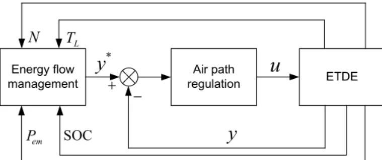
Energy flow

management regulationAir path ETDE

*

y

u

y

N T_L em P SOC

Fig. 2. On-line control diagram of the ETDE

are realistic. In the on-line stage, the air path variables are tuned in the optimization process in two steps. In the energy flow management step, the optimal setpoints of air path variables are calculated so as to minimize fuel consumption. In the air path regulation step, the variables are controlled to track the generated setpoints. The two-step control structure is shown in Fig. 2.

3.1 Energy Flow Management

The primary task of energy flow management is to formu-late the cost function based on fuel efficiency. The total fuel power is

Pa =HLHVWf, (5)

whereHLHV is the lower heating value of the fuel. For

en-ergy is generated from both engine cylinders and battery, the instantaneous equivalent consumed power of an ETDE is given by

Peq=Pa+s(SOC)Pb, (6) where Pb is the battery power, and s(SOC) is a non-dimensional electricity-fuel energy equivalent factor, which applies a necessary penalty on battery state-of-charge (SOC) to discourage pure electric operation.

Since Peq is an instantaneous variable, it can be selected as the cost function

J(y∗) =Peq, (7)

where y∗ denotes the setpoints for controlled variables. The on-line optimization problem is formulated as

min : J(y∗),

s. t : y∗_min≤y∗≤y_max∗ , (8)

where the limits ony∗ denote the permissible range of the setpoints set.

3.2 Air Path Regulation

The objective of air path regulation is the tracking of the computed setpoints y∗. Because the air path is highly nonlinear, it is challenging to build an effective global control strategy that covers all possible operating regions. Developing piecewise-linear controllers at different oper-ating points is a feasible approach, where the operoper-ating points are determined by the independent variables of N

andTL. At a specified operating point, the linear model of the ETDE air path can be expressed in the form of discrete state space equations:

x(k+ 1) =Ax(k) +Bu(k)

y(k) =Cx(k) , (9)

where x ∈ _Rn _{is the state vector,} _u _∈

Rm is the

input vector, y ∈ Rp is the output vector, (A, B) is a

controllable pair, and the coefficient matricesA,B, andC

are obtained via system identification. The entire engine operating region is segregated into several subzones and the identified model at the operating point is effective in the located subzone. The number of subzones depends on the required precision of the identified model.

4. CONTROL-ORIENTED DYNAMICS ANALYSIS The selection of control variables and the boundaries of their setpoints will be underpinned by the dynamics analysis of an ETDE.

4.1 Selection of Control Variables

The key to reducing exhaust emissions in terms of nitrogen oxides (NOx) and particular matter (PM) is keeping

rational values of F1 and λ, which can be obtained from

the independent variablesWcandWegr according to their expressions in Table 1. The independent variables can also be replaced by pin and Wegr. However, to achieve optimal fuel efficiency and exhaust emissions in an ETDE, controlling only pin and Wegr is not enough. Since the EM impacts the exhaust manifold dynamics directly, a further performance variable in the exhaust manifold has to be considered. In the available literature, no explicit principle for selecting control variables of an ETDE and for the analysis of its influence on fuel economy could be found.

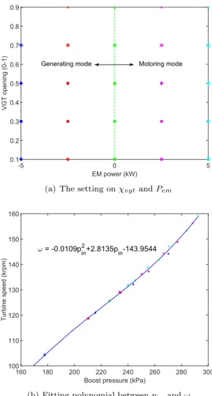
A proposed criterion for selecting control variables is that they must not be strongly coupled. This requirement is necessary for independent control of the selected variables. To analyze the relationship between different control vari-ables, a calibration is implemented on a physical diesel engine model at 1800 rpm, 600 Nm by tuning χvgt and

Pem. The results with no EGR are illustrated in Fig. 3. The setting onχvgtandPem is shown as Fig. 3(a), where

Pem changes from the maximum generating power to the maximum motoring power, with the value of -5 kW and 5 kW, respectively. Theχvgtchanges from 0.1 to 0.9, where 0 implies the VGT vane is fully closed and offers the least flow area to the exhaust flow. Fig. 3(b) shows the strong coupling between boost pressure and turbine speed. The turbine speed behaves as a 2nd-order polynomial function with the boost pressure, which shows the strong coupling between them. On the other hand, the exhaust pressure varies much according to different settings on χvgt, as shown in Fig. 3(c). With the VGT vane closing from 0.9 to 0.1, both boost pressure and exhaust pressure increase, as well as the condition whenPem increases with the fixed

χvgt.

The coupling between boost pressure and turbine speed can also be found using a theoretical causality analysis. Supposing a 2 inputs - 2 outputs control structure, where

pin andω are controlled byχvgt andPem, respectively. If the desired turbine speed ω∗ increases, then Pem would increase accordingly to drive up ω. At the same time,

pin would be driven up because of the enhanced boost assist. To track a steady value ofp∗_in, thenχvgtwould open further to reducepin. As a result, ω is decreased to give a lower pressure ratio in the exhaust manifold. Therefore,

(5)

EM power (kW) -5 0 5 VGT opening (0-1) 0.1 0.2 0.3 0.4 0.5 0.6 0.7 0.8 0.9 Motoring mode Generating mode

(a) The setting onχvgtandPem

Boost pressure (kPa)

160 180 200 220 240 260 280 300 Turbine speed (krpm) 100 110 120 130 140 150 160 ω = -0.0109p_in2+2.8135p_in-143.9544

(b) Fitting polynomial betweenpinandω

160 180 200 220 240 260 280 300

Exhaust pressure (kPa)

200 250 300 350 400 450 500 550 600 χ_vgt=0.1 Pem= -5kW χ_vgt=0.3 P_em= 5kW P_em=0 χ_vgt=0.5 P_em=0 χ_vgt=0.7 Pem=0 P_em=0 χ_vgt=0.9 Pem=0

(c) Calibration data onpinandpexh

Fig. 3. Calibration data by regulating χvgt andPem be selected independently. Based on both test results and dynamics analysis, the control variables are selected as

y= [pin, pexh, Wegr]

T

, (10)

while the control inputs of

u= [χvgt, Pem, χegr]

T

. (11)

4.2 Setting of Boundaries for Setpoints

In the online implementation of energy flow management,

y∗can vary in a range to find the optimal value for best fuel economy. Prior to the online implementation, an offline calibration on the boundaries ofy∗is required to guarantee

y∗ _{are reachable.}

The setpoints of the control variables are denoted as

p∗_in, p∗_exh, and W_egr∗ , respectively. The values of p∗_in and

W_egr∗ can be obtained from the engine calibration settings within the engine control unit (ECU). Therefore, only

p∗_exh is to be determined. A calibration-based approach is implemented to get the boundary values ofp∗_exh, which consists of two steps.

In the first step, a calibration is fulfilled at a specified operating point, followed by the development of a MIMO controller based on the calibration data. In the second step,p∗_exh is set as an incrementally increasing series. The developed MIMO controller is applied on the ETDE model to track p∗_exh. The value of p∗_exh is feasible if it can be tracked well. If the controller fails to track the givenp∗

exh value in some cases, it implies thep∗_exh value is beyond its boundary.

A calibration of the boundary of p∗_exh has been made at 1800 rpm, 700 Nm, while p∗_exh increases from 265 kPa to 289 kPa step-wise, with steps of 2 kPa. Each

p∗_exh value continues for 15 s. Up to 283 kPa, p∗_exh is tracked well. However, strong oscillations happen on all three variables when p∗_exh exceeds the threshold of 283 kPa after 165 s, which means the value of p∗

exh in this period is hard to reach. The spikes onp∗_in and W_egr∗ are due to the ECU generated setpoints being unfiltered. At the very beginning, though 265 kPa can be tracked well, the control inputs especially the EM power are not fully stabilized, which also indicates thep∗_exh value is very close to its lower limit. Therefore, the available range of p∗_exh

is selected as [265 kPa, 283 kPa] at 1800 rpm, 700 Nm. Similarly, the boundaries p∗_exh at other operating points are also determined in the same way. At the other untested operating points, the boundaries are obtained by means of gain scheduling.

5. SUPERVISORY LEVEL CONTROLLER DESIGN The supervisory level controller is designed in the form of ECMS, to minimize fuel consumption while maintaining the battery SOC value. The ECMS realizes the optimiza-tion problem by minimizing an instantaneous cost func-tion, so it behaves as a closed-loop controller. The energy equivalent factor in (6) is designed as

s=KP∆SOC, (12)

whereKP is a positive constant, and

∆SOC = SOC−SOC∗, (13) while SOC∗is the desired value of battery SOC.

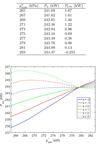
The optimal p∗_exh is obtained from the lookup table ac-cording to the minimal Peq, where the lookup tables are generated from the calibration. The fuel power and EM power with different exhaust pressure settings at 1800 rpm, 700 Nm are listed in Table 2. Without considering electrical energy losses, it is assumed thatPem equals to

(6)

Table 2. Lookup table of Pa and Pem with respect top∗_exh p∗ exh(kPa) Pa(kW) Pem(kW) 265 241.09 1.67 267 241.62 1.61 269 242.05 1.46 271 242.48 1.22 273 242.84 0.96 275 243.16 0.69 277 243.49 0.38 279 243.76 0.06 281 244.09 0.13 283 244.37 -0.255 p_exh* (kW) 266 268 270 272 274 276 278 280 282 Peq (kW) 237 238 239 240 241 242 243 244 245 246 247 s = -2 s = -1 s = 0 s = 1 s = 2 s = 3

Fig. 4. The cost function with respect top∗_exh

cost function Lookup table for Pa * SOC K_P min SOC Lookup table for Pb



b P 0 SOC a P max 1 b Q max b Q b Q * exh p eq P

Fig. 5. The diagram of supervisory level controller

Pb. Based on the data in Table 2, Peq varies with p∗exh ands, as shown in Fig. 4. Whenshas different values, the minimalPeq is represented by differentp∗exh value. The diagram of the supervisory level controller is illus-trated as Fig. 5, where Qb and Qbmax denote the battery

stored energy and battery capacity, respectively. In Fig. 5,

p∗_exh is generated according to the minimized Peq, whose value is computed by the feedback variables Pa and Pb, and the updated cost factors. The generatedp∗_exh is sent to the cascaded low level controller, together withp∗_inand

Wegr∗ from the ECU, as the setpoints to be tracked.

ETDE Controller * in p * exh p * egr W em P vgt  egr  pexh egr W in p

Fig. 6. Control structure of the ETDE

6. LOW LEVEL CONTROLLER DESIGN The single-input single-output (SISO) PI controllers are widely used in the control of conventional turbocharged diesel engines, whilepin andWegr are controlled by χvgt and χegr, respectively. The gain values of PI controllers are generally tuned in off-line calibration. However, in the ETDE, the dynamics has been significantly changed, therefore the controllers require to be re-designed. Since it is time-consuming to re-tune the gain values individu-ally, designing a decoupling MIMO controller is critical. The 3-inputs 3-outputs control structure of the ETDE is illustrated as Fig. 6.

The ETDE model is formed by the state space equations:

"_x_˙ z y # = "_{A B1} _B2 C1 D11 D12 C2 D21 D22 # "_x w u # , (14)

where x, u, and y have been defined in (9). Moreover,

w∈Rm1 _{is the vector of exogenous inputs,}_z_∈

Rp1 _{is the}

vector of regulated outputs.

The dynamic output feedback control law u = K(s)y is to be designed. A nonsmooth H∞ synthesis method is

employed to buildusince it is very convenient in practice, see Apkarian and Noll (2006). This method can address a mixed set of time- and frequency- domain criteria includ-ing settlinclud-ing time, steady state error, stability margin, and noise rejection. The constraints can be grouped as hard (must have) constraints and soft (nice to have) objectives. The controller synthesis is transformed to an optimization problem as minimize g : maxi {kTwi→zi(P, K)k}, (15) subject to : max j { Twj→zj(P, K) } ≤1, (16)

where g is the vector of tunable gain values, kTw→zk denotes the closed loop map from inputwto outputz, and

k·kcan be eitherH∞norm orH2norm,iandjdenote the

index of soft objectives and hard constraints, respectively. The optimization problem (15) and (16) means the mini-mization of the worst-case value of the soft objectives while satisfying all the hard constraints. In the formulation, all terms have been normalized, see Apkarian (2013). In this research, the soft objectives are settling time and steady state error. The hard constraints are stability mar-gins including the gain margin and phase margin. The co-efficient matrices in (14) are obtained via calibration tests. Thesystunesolver in Matlab is adopted to compute the decoupling control law.

7. SIMULATION RESULTS

Simulations have been carried out on a physical plant model built in Dynasty, a proprietary multi physics

(7)

simulation software package used within Caterpillar. The controller and ETDE model are built in Simulink and Dynasty, respectively. The engine manifolds are modeled as one-dimensional components, permitting to capture the pulsations caused by engine actuators operation. All the cylinders are modeled separately to indicate the energy transfer from engine to turbocharger, such that the tran-sient performance is simulated accurately.

The compressor and turbine are represented as map based models. The ETA is also represented as a map-based model, whose maximum motoring/generating power are found from a two-dimensional map, with the inputs of ω

and power electronics controller setting. The controllers are built in Matlab/Simulink for the available tools in Matlab can facilitate the controller design. To guarantee steady communications, the sampling frequency of the controller in Matlab and the controlled plant inDynasty are set as identical. The investigated engine is a CAT six-cylinder, 7.01-Litre heavy duty engine with rated power of 225 kW at 2200 rpm and a rated torque of 1280 Nm at 1400 rpm. The engine has been fitted with an experimental turbo-charger for the purposes of this work. The maps used in the paper are all generated from off-line experimental calibration on the instrumented engine. The battery capacity is set as 0.1 kWh considering the balance between usage flexibility and cost.

The operating points are selected as 1800 rpm, 260 Nm, and 1800 rpm, 700Nm, covering the low load region and high load region, which are typical working conditions in the trenching test cycle for heavy duty engines. A block load condition between the switching of the two operating points is also given, while the gain values are scheduled according to the load.

7.1 Simulation Results of the Low Level Controller

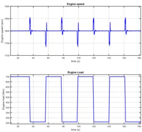
In generating the decoupling control law, the criteria are to be specified. In the soft objectives, the criteria on settling time and steady state error are set as 1s and 0.5%, respectively. In the hard constraints, the criteria on gain margin and phase margin are set as 3dB and 5 rad/s, respectively. The controller is tested under block loads between 1800 rpm, 700 Nm, and 1800 rpm, 260 Nm. The transient period is 1s. The operating conditions are demonstrated in Fig. 7, where the block load condition repeats 4 cycles. In each cycle, the setpoint of pexh at 1800 rpm, 700 Nm is set as 265 kPa, 270 kPa, 275 kPa, and 280 kPa, respectively. Meanwhile, the setpoint of

pexh at 1800 rpm, 260 Nm is kept as 215 kPa in each cycle. The setpoints of pin and Wegr are generated from ECU. The tracking of the control variables in transients is very fast with small spikes, as can be observed in Fig. 8. The decoupling controller only needs to schedule gain values rather than the system model when operating point changes, which reduces the risk of system instability.

7.2 Simulation Results of the Two-Level Controllers

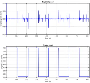
The performance of the two-level controllers in energy management is validated under block loads, while the operating condition is shown as Fig. 9. When the initial values of the battery SOC are set as 20% and 80%,

time (s) 20 40 60 80 100 120 140 160 180 Engine speed (rpm) 1700 1750 1800 1850 1900 Engine speed time (s) 20 40 60 80 100 120 140 160 180 Engine load (Nm) 250 300 350 400 450 500 550 600 650 700 Engine Load

Fig. 7. Operating condition at low level controller test

time (s)

20 40 60 80 100 120 140 160 180

Boost pressure and VGT opening

VGT opening (0-1) 0.1 0.3 0.5 0.7 0.9

Setpoint of boost pressure Boost pressure VGT opening

time (s)

20 40 60 80 100 120 140 160 180

150 200 250 300 350

400 Exhaust pressure and EM power

EM power (kW) -5 -2.5 0 2.5 5

Setpoint of exhaust pressure Exhaust pressure EM power

time (s)

20 40 60 80 100 120 140 160 180

EGR mass flow (kg/s)

EGR mass flow and EGR opening

EGR opening (0-1)

0 0.3 0.6 0.9

Setpoint of EGR mass flow EGR mass flow EGR opening

Fig. 8. Low level decoupling control results at block loads respectively, the tracking performance of control variables, together with the battery SOC convergence are illustrated in Fig. 10 - Fig. 13. The simulation results show that the battery SOC can be driven back to the desired value at both initial conditions. Meanwhile, the updated setpoints of control variables are very well tracked.

8. CONCLUSION

A two-level real-time energy management strategy for the ETDE is proposed in this paper. The control inputs and control outputs are identified based on a concrete control-oriented dynamics analysis of the newly designed electri-fied engine. An explicit principle in setting the boundaries of control variables is also given. A model-based MIMO decoupling controller is designed, while the tracking per-formance under transient conditions and in steady state is fast and smooth. High robustness against the changes on operating conditions is also demonstrated. The super-visory level controller optimizes the fuel economy in real-time, while the sustainable usage of battery is very well guaranteed based on the closed-loop control of battery

(8)

time (s) 0 100 200 300 400 500 600 700 800 Engine speed (rpm) 1700 1750 1800 1850 1900 Engine Speed time (s) 0 100 200 300 400 500 600 700 800 Engine Load (Nm) 250 300 350 400 450 500 550 600 650 700 Engine Load

Fig. 9. Operating condition at two-level energy manage-ment strategy test

time (s)

0 100 200 300 400 500 600 700 800

VGT opening (0-1)

0 0.5 1

time (s)

0 100 200 300 400 500 600 700 800

180 210 240 270

EM power (kW) -2 -1 0 1 2

time (s)

0 100 200 300 400 500 600 700 800

EGR opening (0-1)

0 0.3 0.6

Fig. 10. Two-level energy management results at block loads, with SOC initial value of 20%

SOC. Simulation results demonstrated on a physical en-gine model shows the effectiveness. Verifying the designed energy management strategy on a experimental test bed will be the next step of work.

ACKNOWLEDGEMENTS

This work was co-funded by Innovate UK (formerly the Technology Strategy Board UK), under a grant for the Low Carbon Vehicle IDP4 Programme (TP14/LCV/6/I/BG011L). The Innovate UK is an executive body established by the United Kingdom Government to drive innovation. It promotes and invests in research, development and the exploitation of science, technology and new ideas for the benefit of business - increasing sustainable economic growth in the UK and improving quality of life.

Thanks also go to our consortium partners and subcon-tractors. time (s) 0 100 200 300 400 500 600 700 800 Battery SOC (0 - 1) 0.2 0.25 0.3 0.35 0.4 0.45 0.5 0.55 battery SOC desired battery SOC

Fig. 11. Battery SOC variance with SOC initial value of 20%

time (s)

0 100 200 300 400 500 600 700 800

VGT opening (0-1)

0 0.5 1

time (s)

0 100 200 300 400 500 600 700 800

180 210 240 270

EM power (kW) -2 -1 0 1 2

time (s)

0 100 200 300 400 500 600 700 800

EGR opening (0-1)

0 0.3 0.6

Fig. 12. Two-level energy management results at block loads, with SOC initial value of 80%

time (s) 0 100 200 300 400 500 600 700 800 Battery SOC (0 - 1) 0.4 0.45 0.5 0.55 0.6 0.65 0.7 0.75 0.8 0.85 battery SOC desired battery SOC

Fig. 13. Battery SOC variance with SOC initial value of 80%

(9)

REFERENCES

Apkarian, P. (2013). Tuning controllers against multiple design requirements. In Proceedings of the American Control Conference, 3888–3893.

Apkarian, P. and Noll, D. (2006). NonsmoothH∞

synthe-sis. IEEE Transactions on Automatic Control, 51(1), 71–86.

Arnold, S., Balis, C., Barthelet, P., Poix, E., Samad, T., Hampson, G., and Shahed, S. (2005). Garrett electric boosting systems (EBS) program. Technical Report DE-FC05-00OR22809, Honeywell Turbo Technologies, Rolle, Switzerland.

Bailey, M. (2000). Electrically-assisted turbocharger devel-opment for performance and emissions. In Proceedings of the Diesel Engine Emissions Reduction Workshop, 827803.

Bilgin, B., Magne, P., Malysz, P., Yang, Y., Pantelic, V., Preindl, M., Korobkine, A., Jiang, W., Lawford, M., and Emadi, A. (2015). Making the case for electrified transportation. IEEE Transactions on Transportation Electrification, 1(1), 4–17.

Boyd, D. and Vandenberghe, L. (2010). Technologies and Approaches to Reducing the Fuel Consumption of Medium- and Heavy-Duty Vehicles. The National Academies Press, Washington, D.C., US.

Glenn, B., Upadhyay, D., and Washington, G. (2010). Control design of electrically assisted boosting systems for diesel powertrain applications. IEEE Transactions on Control Systems Technology, 18(4), 769–778. Ibaraki, S., Yamashita, Y., Sumida, K., Ogita, H., and

Jinnai, Y. (2006). Development of the hybrid turbo, an electrically assisted turbocharger. Mitsubishi Heavy Industries Technical Review, 43(3), 1–5.

Terdich, N. and Martinez-Botas, R. (2013). Experimen-tal efficiency characterization of an electrically assisted turbocharger. SAE International, 2013–24–0122. Terdich, N., Martinez-Botas, R., Romagnoli, A., and

Pe-siridis, A. (2014). Mild hybridization via electrification of the air system: Electrically assisted and variable geometry turbocharging impact on an off-road diesel engine. Journal of Engineering for Gas Turbines and Power-Transactions of the ASME, 136(3), 031703. Winward, E., Rutledge, J., Carter, J., Costall, A., Stobart,

R., Zhao, D., and Yang, Z. (2016). Performance testing of an electrically assisted turbocharger on a heavy duty diesel engine. In Proceedings of the 12th International Conference on Turbochargers and Turbocharging. Yang, Z., Winward, E., Zhao, D., and Stobart, R. (2016).

Three-input-three-output air path control system of a heavy-duty diesel engine. InProceedings of the 8th IFAC International Symposium on Advances in Automotive Control.

Zhao, D., Liu, C., Stobart, R., Deng, X., E., W., and Dong, G. (2014). An explicit predictive control framework for turbocharged diesel engines. IEEE Transactions on Industrial Electronics, 61(7), 3540–3552.

Zhao, D., Liu, C., Stobart, R., Deng, X., Winward, E., and Dong, G. (2013). Explicit model predictive control on the air path of turbocharged diesel engines. In

Proceedings of the American Control Conference, 5220– 5225.

Zhao, D. and Stobart, R. (2015). Systematic control on energy recovery of electrified turbocharged diesel

engines. In Proceedings of the 54th IEEE Conference on Decision and Control, 1527–1532.

Zhao, D., Stobart, R., Dong, G., and Winward, E. (2015). Real-time energy management for diesel heavy duty hybrid electric vehicles. IEEE Transactions on Control Systems Technology, 23(3), 829–841.

Zhao, D., Winward, E., Yang, Z., and Stobart, R. (2016). Control-oriented dynamics analysis for electrified tur-bocharged diesel engines. In SAE Technical Paper, 2016–01–0617.