Strathprints Institutional Repository
Zabalza, Jaime and Ren, Jinchang and Zheng, Jiangbin and Han, Junwei
and Zhao, Huimin and Li, Shutao and Marshall, Stephen (2015) Novel two
dimensional singular spectrum analysis for effective feature extraction
and data classification in hyperspectral imaging. IEEE Transactions on
Geoscience and Remote Sensing, 53 (8). pp. 4418-4433. ISSN 0196-2892 ,
http://dx.doi.org/10.1109/TGRS.2015.2398468
This version is available at http://strathprints.strath.ac.uk/53408/
Strathprints is designed to allow users to access the research output of the University of Strathclyde. Unless otherwise explicitly stated on the manuscript, Copyright © and Moral Rights for the papers on this site are retained by the individual authors and/or other copyright owners. Please check the manuscript for details of any other licences that may have been applied. You may not engage in further distribution of the material for any profitmaking activities or any commercial gain. You may freely distribute both the url (http://strathprints.strath.ac.uk/) and the content of this paper for research or private study, educational, or not-for-profit purposes without prior permission or charge.
Any correspondence concerning this service should be sent to Strathprints administrator:
Abstract—Feature extraction is of high importance for effective data classification in hyperspectral imaging (HSI). Considering the high correlation among band images, spectral-domain feature extraction is widely employed. For effective spatial information extraction,
a 2-D extension to singular spectrum analysis (SSA), a recent technique for generic data mining and temporal signal analysis, is proposed.
With 2D-SSA applied to HSI, each band image is decomposed into varying trend, oscillations and noise. Using the trend and selected oscillations as features, the reconstructed signal, with noise highly suppressed, becomes more robust and effective for data classification.
Three publicly available data sets for HSI remote sensing data classification are used in our experiments. Comprehensive results using a
support vector machine (SVM) classifier have quantitatively evaluated the efficacy of the proposed approach. Benchmarked with several state-of-the-art methods including 2-D empirical mode decomposition (2D-EMD), it is found that our proposed 2D-SSA approach
generates the best results in most cases. Unlike 2D-EMD which requires sequential transforms to obtain detailed decomposition, 2D-SSA
extracts all components simultaneously. As a result, the executive time in feature extraction can also be dramatically reduced. The superiority in terms of enhanced discrimination ability from 2D-SSA is further validated when a relatively weak classifier, k-nearest
neighbor (k-NN), is used for data classification. In addition, the combination of 2D-SSA with 1D-PCA (2D-SSA-PCA) has generated the
best results among several other approaches, which has demonstrated the great potential in combining 2D-SSA with other approaches for effective spatial-spectral feature extraction and dimension reduction in HSI.
Index Terms—Data classification, feature extraction, hyperspectral imaging (HSI), 2-D empirical mode decomposition (2D-EMD), 2-D singular spectrum analysis (2D-SSA).
I. INTRODUCTION
yperspectral imaging (HSI) provides data captured in a 3-D structure, namely a hypercube, which contains 1-D spectral
Manuscript received July 4, revised November 6 2014.
J. Zabalza, J. Ren* (Corresponding author), and S. Marshall are all with Centre for excellence in Signal and Image Processing, Dept. of Electronic and Electrical Engineering, University of Strathclyde, Glasgow, U.K. (Emails: [email protected],
[email protected], [email protected]).
J. Zheng is with School of Computer Software and Microelectronics, Northwestern Polytechnical University, China. (Email:
J. Han is with School of Automation, Northwestern Polytechnical University, China. (Email: [email protected]). H. Zhao is with College of Electronics and Information, GDIN, China. (Email: [email protected]).
S. Li is with College of Electrical and Information Engineering, Hunan University, China. (Email: [email protected]).
Jaime Zabalza, Jinchang Ren, Jiangbin Zheng, Junwei Han,
Huimin Zhao, Shutao Li, and Stephen Marshall
Novel Two Dimensional Singular Spectrum Analysis
for Effective Feature Extraction and Data
Classification in Hyperspectral Imaging
information along with a 2-D spatial scene. With spectral information continuously acquired over a long range from visible spectrum to (near) infrared, HSI is able to identify minor object difference in terms of moisture, temperature and chemical components. As a result, HSI has become a research hotspot in recent years and has been successfully applied in many applications. These include not only conventional remote sensing, military surveillance and mining but also new emerging lab-based data analytics tasks such as forensics, pharmaceutical, medical and food quality analysis [1-4].
Considering the fact that each pixel in HSI naturally forms a spectral vector, i.e. spectral profile, pixel-based data analysis is widely used for object detection and data classification. In HSI, pixels can be easily characterized by using the corresponding spectral profile, where support vector machine (SVM) has been widely adopted to identify their differences even unnoticeable to our naked eyes [5-7]. As HSI presents high correlation among spectral bands, this makes feasible the dimensionality reduction of features. To this end, feature extraction and feature selection in the spectral domain are also emphasized regarding both the curse of dimensionality, also known as Hughes effect [8] and the reduction in computational complexity.
With the strong demands from remote sensing and other related applications, feature extraction and dimension reduction in HSI has been intensively investigated in the last decades. Some widely-used methods include principal component analysis (PCA) [9] and several variants [10-12], maximum noise fraction (MNF) [13-14], and independent component analysis (ICA) [15-16]. Other interesting approaches comprise band selection [17], steepest ascent [5, 18] and machine learning based approaches [6-7]. Furthermore, the extensive HSI literature offers more techniques such as Bhattacharyya and Jeffries-Matusita distances, spectral angle mapper, mutual information, vegetation index NVDI, linear discriminant analysis, decision boundary feature extraction, non-parametric weighted feature extraction, or even discrete wavelet transform [19]. A general overview of those methods and some comparisons can be found in [19-21].
However, in the recent years, the limited contribution of spectral-domain feature extraction in combination to the potential use of spatial information has been highlighted, where spatial processing techniques have been proposed for improved classification accuracy [22-23]. The first group of such spatial processing approaches is spatial filtering, including mathematical morphology processing and median filtering, where spatial-domain feature extraction is achieved by applying either opening/closing operators or median filtering to the images [22-24, 25]. In [22], morphological processing is applied to one PCA component of the HSI data, namely the morphological profile (MP) technique. In [23], MP approach is extended to include several few PCA components, leading to the extended morphological profile (EMP) method, whose performance is evaluated with a SVM classifier in [24]. Nevertheless, the performance of morphology processing is highly dependent on the size and shape of the associated structure element, regardless the variations in terms of the number of openings/closings (and PCA components) to be employed in EMP. In [25], an adaptive filter (AF) using median filtering and MNF is presented for feature extraction in HSI, in which a kernel size that is
inversely related to the signal-to-noise ratios (SNRs) of the MNF bands is used. Among several variants introduced, AF with derivate (AFD) seems to perform the best. However, its performance, depending on the MNF, suffers from significantly degraded signal quality and affects by the kernel size which is not clearly explained.
Another interesting group of method is 2-D empirical mode decomposition (2D-EMD) [26] based approaches. As the key part of the Hilbert Huang transform (HHT), EMD has been used for the analysis of non-linear and non-stationary time series [27-28]. Being able to decompose a signal into several and usually a few components known as intrinsic mode functions (IMFs), EMD is originally applied for applications of 1-D signal, such as speech recognition [29]. To deal with 2-D images, its extension, 2D-EMD has been proposed [26, 30-31]. In 2D-EMD, each image or band image within a hypercube is reconstructed using the lower-order IMFs extracted components whilst discarding the remaining ones, simply because these lower order IMFs present the spatial structure of the scene while higher order IMFs lack this content [26]. Accordingly, using the reconstructed hypercube for data classification can significantly improve the efficacy and surpass many state-of-the-art approaches [26]. On the other hand, the whole process for 2D-EMD implementation is based on iterations and becomes very computational expensive, resulting unfeasible in some cases.
Also there are some other spatial-domain techniques proposed in the recent literature. In [32], unsharp filtering is applied to enhance the high frequency content in an image and boost edges of the different elements in the scene. In [33-34], wavelet decomposition of images is utilized for spatially-adaptive image denoising and results in an increment of accuracy in HSI classification. However, these techniques seem to provide limited improvement in classification accuracy as 2D-EMD does [26]. On the other hand, it is important to remark the potential applications where spatial information is employed for post-processing of already classified data. In [35], texture and morphological features are combined with the MNF technique to refine the data classified using SVM and a fuzzy neural network. The evaluation has shown that both texture and morphological features make limited contributions in the experiments, which indicates that spatial features should be more favourable introduced before the classification stage.
In this paper, we focus on the singular spectrum analysis (SSA) [36], a promising data mining technique which has been applied in 1-D (1D-SSA) in the spectral domain and shown great potential for effective feature extraction in HSI [37-38]. With the profile of a given pixel vector being decomposed into several components, SSA can help easily remove the noisy components thus enhance the signal for improved data classification. Being based on the well-known singular value decomposition (SVD), 1D-SSA is able to beat other relevant techniques in terms of classification accuracy [37-38], becoming of great interest for feature extraction in the spectral domain. However, considering the fact that spatial features can also significantly improve the accuracy of classification [20, 26], we have naturally proposed the idea to extend 1D-SSA to 2-D analysis. In addition, existing techniques working in the spatial domain can only deal with spatial relationship within a small neighborhood (window), even in certain shapes subject to the defined structure
elements and filter templates in morphological processing and median filtering. For example, EMP simply applies opening and closing operators to the images, and the AFD uses a basic median filter, hence the improvement from these methods tend to be limited and sometimes even inconsistent.
To address these drawbacks, we propose the extended 2-D version of SSA (2D-SSA) to fully explore the spatial correlation of HSI images. Based on the well-known SVD theory, the 2D-SSA aims to provide a systematic solution for spatial feature extraction in HSI. Actually, similar approaches in 1-D cases, including PCA (and 1D-SSA), have already been widely used in HSI feature extraction and data reduction though being applied in spectral domain. As components can be extracted from SVD in one transform, 2D-SSA needs no iterative process as 2D-EMD does in signal decomposition and results in significantly reduced computational cost for improved efficiency. The proposed 2D-SSA method has been especially benchmarked with 2D-EMD [26], and also with a number of other state-of-the-art approaches, where excellent results in classification accuracy have been generated, surpassing the rest of techniques normally used in this context yet requiring much less execution time than 2D-EMD.
The remaining part of this paper is organised as follows. Section II describes the original SSA algorithm, including the concept, mathematical background and a practical example. Section III focuses on the proposed 2D-SSA extension for feature extraction in HSI. Section IV discusses detail about experimental setup, including data sets and parameters settings. Experimental results and quantitative analysis are presented in Section V, with some concluding remarks drawn in Section VI.
II. PRINCIPLES OF SSA
As a novel technique for time series analysis and forecasting, SSA has been successfully applied in climatic, meteorological, and geophysical applications as well as generic data mining in social science [36]. Based on some earlier work [39-40], SSA has attracted increasing attention with remarkably theoretical and practical progress reported in recent years [36, 41-42]. In one of our previous papers [38], applying SSA to the HSI pixels for effective feature extraction and data classification is evaluated, proving its efficacy and great potential in this context. In the following, detailed information about the SSA, its concept and the algorithm along with a practical example are presented.
A. Concept
Based on SVD, SSA is able to decompose an original series into several independent components or subseries, where every Eigenvalue extracted from the original series provides an individual component. Moreover, these individual components can be grouped to produce others that may be interpretable as varying trend, oscillations or noise. Accordingly, the main capabilities of SSA can be summarized as follows [41]:
2) extraction of periodic components;
3) complex trends and periodicities with varying amplitude; 4) finding structures in short time series;
5) envelopes of oscillating signals.
How to handle specific components of the decomposed signal, especially those related to noise, has made SSA a promising technique still to be evaluated in many fields.
B. Algorithm
Assume that we have a HSI pixel, being a 1-D signal in a vector array
p
defined asp
[
p
1,
p
2,
,
p
N]
N; the SSAalgorithm can be applied in the following steps. 1) Embedding
Defining a window size
L
Z
satisfyingL
[
1
,
N
]
, the trajectory matrixX
of the vectorp
can be constructed as
K
N L L K Kp
p
p
p
p
p
p
p
p
c
c
c
X
1,
2,
,
1 1 3 2 2 1
. (1)Each column of
X
,c
k , is a lagged vector which can be represented asc
k
[
p
k,
p
k1,
,
p
kL1]
T
L , where]
,
1
[
K
k
andK
N
L
1
. It is worth noting that the matrixX
has equal values along the anti-diagonals, thus it is actually a Hankel matrix by definition.In fact, based on a property of the matrix
X
[41], the SSA algorithm can be implemented symmetrically in two intervals:)]
2
/
(
,
1
[
round
N
L
andL
[
ceil
((
N
1
)
/
2
),
N
]
, whereround
andceil
operators represent the rounding and ceiling functions in computer science. For a givenL
, the equivalent implementation can be found for anotherL
'
K
, leading to the same results. In addition, just remark that both singular ends from the global interval,1
andN
, do not provide a SSA implementation.2) Singular Value Decomposition (SVD)
First the matrix
S
is obtained from the trajectory matrixX
asS
X
X
T. The Eigenvalues ofS
and their corresponding Eigenvectors are then denoted respectively as
1
2
L
and
u
1,
u
2,
,
u
L
.For the trajectory matrix
X
, its SVD is then formulated as given below. Though the value ofd
L
equals to the rank ofX
, from now on we considerd
L
for simplicity, i.e.,L
X
X
X
X
1
2
. (2) As can be seen, the trajectory matrixX
is actually built by the addition of several matrices. Each matrixX
l|
l
[
1
,
L
]
is called elementary matrix, corresponding to its respective Eigenvalue as defined byT l l l l
u
v
X
(3) wherev
l is defined as l l T l
u
X
v
. (4)Note that the collection
l,
u
l,
v
l
is normally called the lth eigentriple, and the matricesU
andV
below are denoted as the matrix of empirical orthogonal functions and the matrix of the principal components, respectively, i.e.,
K L L L L L
v
v
v
V
u
u
u
U
,
,
,
,
,
,
2 1 2 1
. (5) 3) GroupingIn this step, the total set of
L
components is divided intoM
disjoint setst
1,
t
2,
,
t
M , where
|
t
m|
L
and]
,
1
[
M
m
. Lett
l
1,
l
2,
,
l
q
denote one of the divided sets, the matrixX
t related to the groupt
is defined asq l l l
X
X
X
X
t
21 . Finally, the trajectory matrix
X
is represented byM t t t
X
X
X
X
2 1 . (6)For simplicity, a typical grouping is the one such as
M
L
, i.e.,q
1
, which refers to the case that each set is made of just one component. In general, the contribution of each matrixX
t to the trajectory matrixX
in the SVD is related to its Eigenvalues and therefore can be derived as
L l l l l 1
t t . (7)4) Diagonal Averaging The matrices
,
m
[
1
,
M
]
m
t
X
obtained above by grouping are not necessarily the Hankel type as in the original trajectory matrix. However, in order to project each of these matrices into 1-D signal, they have to be hankelized. This step is done by obtaining the average in all the anti-diagonals of eachm
t
X
, simply because these values used for average contribute to the sameelement in the derived 1-D vector array.
Let
z
m
[
z
m1,
z
m2,
,
z
mN]
N denote the 1-D signal projected fromX
tm, it can be obtained via diagonal averaging below, wherea
r,nr1 refers to the elements ofm t
X
, i.e.,
N
n
K
a
n
N
K
n
L
a
L
L
n
a
n
z
L K n r r n r L r r n r n r r n r mn 1 1 , 1 1 , 1 1 ,1
1
1
1
1
. (8)With the obtained
z
m above, the original 1-D signalp
can be reconstructed by
M m m M 1 2 1z
z
z
z
p
. (9)As a result, the original signal can also be represented using one or more groups derived from its Eigenvalues, where those less significant components or highly noisy ones are discarded.
C. Example of SSA Application in HSI
In HSI, the original profile over the spectral domain of one pixel in the scene can be decomposed according to the Eigenvalues extracted in its SVD. Therefore, it is possible to substitute the original pixel by a more significant profile, reconstructed in such a way with the contribution of the smaller eigencomponents being ignored [38].
An effective replacement of the original profile is decided by two key parameters. The first one is the window size L, which determines the total number of Eigenvalues that can be extracted in the decomposition stage. A window size L=10 provides 10 components, one per each Eigenvalue in its SVD. The addition or grouping of those components leads to a particular reconstruction, taking into account that the profile corresponding to the first Eigenvalue is much more significant than those corresponding to the following ones.
The second parameter is what we call the Eigenvalue grouping (EVG), which describes how the extracted components are grouped in reconstructing the original signal. If the EVG includes all Eigenvalues, the reconstruction is equivalent to the original
profile. If the EVG excludes the components from the smallest Eigenvalues, the reconstructed profile is probably less noisy, as noise is usually contained in these small Eigenvalues. Finally, if the EVG leaves out the component from the first Eigenvalue, the reconstruction is not appropriate as it losses the main information provided by the original signal.
An example of SSA application is given in Fig. 1, where the original profile and the reconstructed signal with the parameters L=5 and EVG=1st are plotted. As only the first Eigenvalue component is selected in reconstructing the signal, the resulting profile preserves the basic trend. In addition, avoiding less representative Eigenvalue components can potentially reduce noise content in the new profile, leading to a better feature extraction and classification results [38].
0 50 100 150 200 1000 2000 3000 4000 5000 6000 Spectral bands M a g n it u d e Original profile Reconstructed profile
Fig. 1. Original and reconstructed (by SSA) profiles for one pixel in HSI. The reconstruction is derived from the first Eigenvalue component out of five.
III. EXTENSION TO 2D-SSA FOR ANALYZING HSI
Though the original 1D-SSA can be used for HSI analysis with improved classification accuracy reported [38], its pixel-level implementation results in negligence of spatial relationship among the pixels, where only spectral correlation is addressed. As spatial features can also lead to improved data classification [26], we propose the introduction of 2D-SSA for HSI spatial-domain feature extraction. Although some recent work has been reported using 2D-SSA in some applications [43-47], applying 2D-SSA for effective feature extraction and data classification in HSI has been seldom addressed. In this section, the concept of 2D-SSA, with mathematical description and examples of application are provided for an easy understanding.
A. Concept
In general, 2D-SSA is similar to 2D-EMD in HSI analysis. When the 2D-EMD is applied to each spectral band of a hypercube, it reconstructs the 2-D spatial scene with the low order IMFs. This is because low order IMFs reflect the spatial structural content while high order IMFs lack local spatial structure [26, 30]. Analogously to the 2D-EMD approach, 2D-SSA also aims to extract spatial information as reflected in the first Eigenvalue components. Based on the SVD, the reconstruction of each spectral band
image using its respective main components leads to spatial structural content extraction whilst noise, normally located in the small Eigenvalue components, can be removed or suppressed simultaneously.
B. Algorithm
When implementing SSA over a 2-D signal, basically the SVD and grouping steps are identical as in the 1-D case, and only the embedding and diagonal averaging stages have to be adapted.
1) Embedding a 2-D Signal
For an image
P
2D with a sizeN
x
N
y, its matrix representation is given as followsy x y x x x y y N N N N N N N N D
p
p
p
p
p
p
p
p
p
, 2 , 1 , , 2 2 , 2 1 , 2 , 1 2 , 1 1 , 1 2
P
. (10)Similar to the 1-D case, a window needs to be defined for the construction of the trajectory matrix. However, the difference here is that in 2D-SSA the window moves over an image rather than a 1-D vector. In other words, a 2D-window is needed in 2D-SSA, which is usually represented using the position of its top-left corner
i
,
j
as given below, where the size of the window isL
x
L
y withL
x
[
1
,
N
x]
andL
y
[
1
,
N
y]
y x y x x x y y L L L j L i j L i j L i L j i j i j i L j i j i j i j ip
p
p
p
p
p
p
p
p
1 , 1 1 , 1 , 1 1 , 1 1 , 1 , 1 1 , 1 , , ,
W
. (11)In the same way as in the 1-D case, a symmetric and equivalent implementation can also be found in 2D-SSA delimited approximately by
N
x/
2
andN
y/
2
forL
x andL
y, respectively. Within the same dimensions inL
x andL
y, the 2-D windowcan also be defined as
T L j r i j r i j r i j i j i j i j i j i y r x L
p
p
p
1 , 1 1 , 1 , 1 ) , ( ) , ( ) , ( ) , ( , 2 1
w
w
w
w
W
. (12)To construct the trajectory matrix, the window
W
i,j has to be placed in all possible positions over the imageP
2D. The path to follow by the window is raw-scanning from the top-left to the bottom-right of the image, given in relation to its reference point
i
,
j
wherei
[
1
,
N
x
L
x
1
]
andj
[
1
,
N
y
L
y
1
]
. A total of
N
x
L
x
1
N
y
L
y
1
possible positions of the window are located in the image.At a given reference point
i
,
j
, the corresponding 2-D window is rearranged into a column vector asy x y x y x L L L L j L i j i L j i j i j i T j i T j i T j i j i
p
p
p
p
p
1 , 1 , 1 1 , 1 , , ) , ( ) , ( ) , ( , 2 1
w
w
w
A
. (13)And the trajectory matrix
X
2D can be derived by) 1 )( 1 ( 1 , 1 1 , 2 1 , 1 2 , 1 1 , 1 2
x y x x y y y y x x y y L N L N L L T T L N L N T T L N T T DA
A
A
A
A
X
. (14)The obtained trajectory matrix
X
2D has a structure called Hankel-block-Hankel (HbH), which is not exactly the same as but related to a basic Hankel matrix. In fact, the HbH matrixX
2D can be represented as) 1 ( 1 2 3 2 1 2 1 2
x x x x x x x x x x L N L N L L L N L N DH
H
H
H
H
H
H
H
H
X
(15)) 1 ( , 1 , , 2 , 3 , 2 , 1 , 2 , 1 ,
y y y y y y y y y y L N L N r L r L r L N r r r L N r r r rp
p
p
p
p
p
p
p
p
H
. (16)Note that an HbH matrix (
X
2D) is Hankel in block terms, being each one of the blocks (H
r) Hankel by itself. These considerations have to be taken into account especially at the last stage of 2D-SSA algorithm.2) Singular Value Decomposition (SVD) and Grouping
These two central stages are exactly the same as those in original SSA algorithm. However, the respective dimensions need to be changed when the algorithm is adapted to 2-D cases. Specifically, we have
K
2D
N
x
L
x
1
N
y
L
y
1
andy x D
L
L
L
2
. In addition, the problem derived from what grouping is appropriate is discussed in Section IV.C.
3) Diagonal Averaging
Similar to the 1-D case, the matrices D
m
2
t
X
obtained by grouping in 2D-SSA are also not necessarily HbH type. As a result, they need be transformed to HbH matrices, and this can be done by means of a two-step hankelization process as given below.For the averaging procedure, two sequential hankelizations are needed, firstly applied within each block (16), and then applied between blocks (15). Again, an average among the values contributing to the same element in the image is carried out, so now
Z
m2Dis the 2-D signal projected from group D
m 2 t
X
y x y N x N x N x N y N y N N N m m m m m m m m m D mz
z
z
z
z
z
z
z
z
, 2 , 1 , , 2 2 , 2 1 , 2 , 1 2 , 1 1 , 1 2
Z
. (17)Note that the original 2-D image in (10) can be represented as
M m D m D M D D D 1 2 2 2 2 2 1 2Z
Z
Z
Z
P
. (18)Accordingly, this enables to decompose an image into several components extracted
Z
m2D based on SVD. Each component is related to each Eigenvalue in the SVD, and therefore the appropriate grouping of components leads to a reconstruction of the original image, where spatial structural content is extracted while noise, usually located in small Eigenvalues, is avoided.C. Example of 2D-SSA Application in HSI
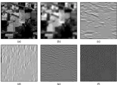
In HSI, each spectral band of the hypercube forms a 2-D image, where the information contained in the spatial domain provides useful clues for data classification. For a randomly selected spectral band, at 667 nm, the original band image and the extracted scenes derived from the Eigenvalues content in 2D-SSA are shown in Fig. 2. As can be seen, detailed spatial features can be observed in the extracted 2D-SSA components with local structure preserved. On the other hand, noise can be removed by excluding components from small Eigenvalues. Therefore, an original band image can be decomposed and then reconstructed by few main components. Applying this process to all the spectral bands, the original hypercube can be represented by a combination of the 2D-SSA components rather than the original band images, where the preserved local structure and removed noise can potentially lead to better classification of pixels inside the images.
(a) (b) (c)
(d) (e) (f)
Fig. 2. Application of 2D-SSA to a scene in HSI. (a) Original scene at 667 nm (b) First (c) Second (d) Third (e) Fourth individual components and (f) Grouping by the rest of components from 5-25th, where Lx=5, Ly=5 (L2D=25).
In 2D-SSA, same as in the 1-D case, the effectiveness of the approach is also affected by two key parameters, i.e., the dimension of the window in data embedding, and the number of components used in representing the original image. In fact, the total number of Eigenvalues (components) available is determined by the dimension of the window implemented in the embedding stage. For example, in a case with Lx=5 and Ly=5, L2D equals to 25, which is the total number of components available from the decomposition of the original scene that can be used in reconstructing the scene.
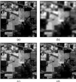
In Fig. 3, examples in reconstructing one band scene of a hypercube using various numbers of components are compared. With more components used, the reconstructed scene becomes more similar to the original one. Obviously, the grouping made from 1-L2Dth components, where L2D=Lx×Ly, gives as a result the same original scene. However, a smaller grouping from 1-10th components already makes the resulting image unnoticeably different from the original one.
(a) (b)
(c) (d)
Fig. 3. Application of 2D-SSA to a scene in HSI. (a) Original scene at 667 nm (b) First component grouping (c) From first to fifth component grouping (d) From first to tenth component grouping , where Lx=5, Ly=5 (L2D=25).
One of the main differences of 2D-SSA in relation to original SSA is, from our point of view, the extraction of main trend and local structure over the spatial domain, which increases the discrimination ability for data classification. To this end, not only the noise removal by discarding the contribution of small Eigenvalues increases the potential of higher classification accuracy, but moreover, the spatial structures in an image are taken into account as an improvement to the extracted features.
Initially, the 2D-SSA method is thought, for simplicity, to compute in the same way all the images along the spectral domain in a hypercube, that is, the different stages are implemented for the different spectral scenes using the same parameters value. Further research is ongoing to evaluate a different parameters value implementation based on the spectral content of the scene found in a hypercube.
D. Applying 2D-SSA to non-HSI images
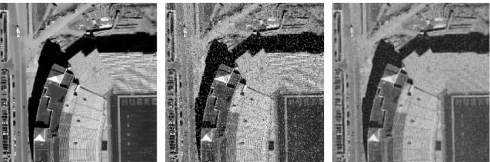
Although 2D-SSA is proposed here for feature extraction in HSI, it can also be applied to non-HSI images for denoising and feature extraction. First, a spectral band of the image ‘memorial stadium’ (high resolution of 0.15 meter-pixel) [48] is used for denoising test, where the top-left 600x600 portion of the image is shown in Fig. 4 for easy visualization. Salt-and-pepper noise is randomly added to 10% of the pixels. Then, the noisy image is treated with the 2D-SSA technique (Lx=Ly=10, selecting from 1st to
10th components). Simply by comparing the SNR, it is proved that the noisy image treated by 2D-SSA is enhanced (34.3 dB) in relation to the original noisy image (21.2 dB).
Fig. 4. One original image (left), its noisy version with salt-and-pepper noise (middle), and 2D-SSA treated image (right) with parameters (Lx=Ly=10, selecting
from 1st to 10th components).
Second, an example in feature extraction is also tested and shown in Fig. 5. On one hand, we extract the main trend of the image, i.e. the 1st component where again we use Lx=Ly=10. As can be seen, 2D-SSA homogenizes different elements in the scene, making
it more uniform in shape and content. On the other hand, using a different configuration for 2D-SSA (Lx=Ly=10 and the remaining
9 components for reconstruction), the structural shape delimiting different elements can be extracted with great detail, which also proves the capability of 2D-SSA for detecting small targets in an image.
Fig. 5. One original image (left), main spatial trend extracted by 2D-SSA (middle) with parameters (Lx=Ly=10, 1st component), and detailed structure extracted
by 2D-SSA (right) with (Lx=Ly=10, 2nd to 10th components).
IV. EXPERIMENTAL SETUP
Experimental settings are organized in four stages including data description, data conditioning, feature extraction, and data classification. All the algorithms are implemented in Matlab environment. Detailed descriptions of the data and relevant algorithms for benchmarking are presented below.
A. Data Description
Three remote sensing data sets with available ground truth are employed in our experiments to quantitatively evaluate the effectiveness of the extracted features in data classification. These data sets are subscenes extracted from their original scenes [49-50], collected using different instruments which are well-known in the remote sensing field.
The first data set is 92AV3C, also known as Indian Pine, collected by using the Airborne Visible/InfraRed Imaging Spectrometer (AVIRIS) [51] over an agricultural study site in Northwest Indiana, USA. This data set is widely used in remote sensing
applications, which contains 224 contiguous bands with a spectral range from 400 to 2500 nm. As shown in Fig. 6, it has 145×145 pixels in 220 spectral bands for land usage purpose, after removing 4 invalid bands degraded by severe noise. It contains 16 labeled land cover classes, mostly related to agriculture, forest and perennial vegetation. However, for consistency with related research [5-7, 26], in total 7 classes were discarded due to the small number of samples available for experiments, resulting in only 9 classes used for quantitative assessment.
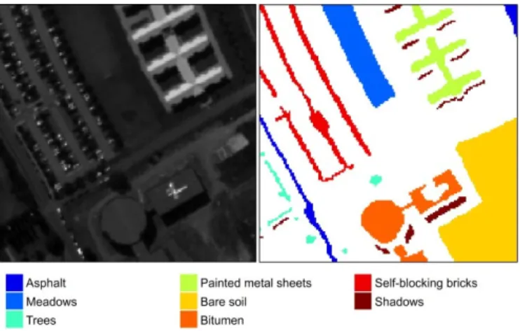
The second data set is the Pavia University A (Pavia UA), taken in North Italy using the Reflective Optics System Imaging Spectrometer (ROSIS) [52]. The sensor provides in this case 114 bands with a spectral range between 430 to 860 nm. This is a subscene made of 150×150 pixels, as shown in Fig. 7, providing a spatial resolution of 1.3 m. In total 8 classes such as meadows, asphalt, trees, and others are contained in its ground truth map.
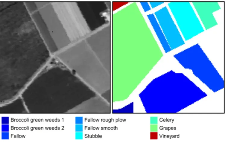
Finally, the third data set, Salinas C, is also acquired using the AVIRIS spectrometer [51]. As shown in Fig. 8, this data set is a subscene taken over the Salinas Valley in California, USA, which has 150×150 pixels in 224 spectral bands, presenting a spatial resolution of 3.7 m. The ground truth map contains 9 classes corresponding mainly to broccoli, fallow, and grapes among others.
Fig. 6. One band image at the wavelength of 667 nm (left) and the ground truth map for the 92AV3C data set (right).
Fig. 8. One band image at the wavelength of 667 nm (left) and the ground truth map for the Salinas C data set (right).
B. Data Conditioning
HSI data acquisition is usually affected to some degree by different sources of noise. To this end, the starting hypercubes [49-50] are subject of a conditioning process where some data is removed before any analytical tasks. In the spectral domain, depending on the corresponding wavelength, some bands can be severely affected by water absorption, noise or other effects. Accordingly, certain bands are usually discarded by visual inspection as recommended by others [7, 50], reducing the available number of bands from 220 to 200, 114 to 103 and 224 to 204 for the 92AV3C, Pavia UA and Salinas C data sets, respectively.
In relation to the spatial domain of the hypercubes, as already mentioned in the data description, for the well-known 92AV3C data set several authors suggest to remove those classes presenting a small number of pixels in the ground truth [5-7, 26], claiming a higher statistical significance in the results. Although we achieve similar results using all 16 classes, 92AV3C is evaluated only for 9 classes in order to guarantee a consistent comparison with others. Pavia UA and Salinas C data sets maintain all ground truth classes in their analysis.
C. Feature Extraction
As feature extraction can significantly affect the accuracy of data classification, this stage is very important in the signal processing chain. In [26], 2D-EMD technique was introduced, where its classification accuracy surpassed all other relevant methods in this context, giving an excellent efficacy. However, the main drawback of 2D-EMD is its extremely high computational complexity [26].
As a result, 2D-EMD [26] is used as main benchmarking approach in our paper, along with the conventional 1D-SSA technique [38] from which 2D-SSA is extended. Also the use of original spectral values from the pixels as features (or absence of feature extraction method) is taken as a Baseline for performance assessment. The efficacy and efficiency of these approaches are compared with our proposed 2D-SSA method. As shown in the next section, 2D-SSA is able to provide similar efficacy as 2D-EMD but requiring a much reduced time for implementation.
These methods and parameters used are summarized in Table I, where the Baseline case is straight as it requires no parameters, while for the 1D-SSA method we use the same configuration implemented for the main results in [38]. For the 2D-EMD implementation in Matlab, initially we evaluated the publicly available code in [53]. However, this Matlab implementation in practical terms is infeasible as it takes a really amount of time in the code execution, especially for large data sets in HSI. As a result, a more suitable version of 2D-EMD code from [54] is used in our study, as it is found that this code is appropriate for an evaluation of 2D-EMD and subsequent comparison with the 2D-SSA algorithm. The selected code uses a stop criterion based on the normalized mean square error, with a recommended threshold value of =0.2, which is experimentally proved to guarantee an effective capture of the 2-D IMF signals. Finally, a total of four different combinations made by the first, the first to the second, the first to the third, and the first to the fourth IMFs groupings are evaluated as in [26].
TABLEI
MAIN EVALUATED IMPLEMENTATIONS FOR FEATURE EXTRACTION
Method Parameters Values adopted
Baseline N/A N/A
1D-SSA [38] Window L 5, 10
EV Grouping (EVG) 1st, 1-2nd
2D-EMD [26]
Stop threshold 0.2 IMF Grouping (IMFG) 1st, 1-2nd, 1-3rd and 1-4th 2D-SSA Window L
2D (L
x×Ly) 5×5, 10×10, 20×20, 40×40, and 60×60
EV Grouping (EVG) 1st, 1-2nd, 1-5th, and 1-10th
For the 2D-SSA method, implementation of the algorithm described in Section III is easily carried out also in Matlab environment. This method depends on two parameters, the window size L2D=Lx×Ly and the EV grouping used for the reconstruction. According to Golyandina et al [36], these parameters values must be selected based on the properties of the original data set and the purpose of the analysis.
Normally, the parameters value selection is similar to that in 1-D cases [36, 38, 47], though the extraction of structures in the spatial domain needs be considered. In general, for a fixed EV grouping, the implementation with a small window leads to good reconstructions of the image, as a larger window may produce too smoothed results and cause a mixing problem [47]. Also, symmetry property [41] of the trajectory matrices fixes the available implementation range in [2, Nx/2] and [2, Ny/2] for Lx and Ly, respectively, and the selection of values Lx≠Ly derives in a non-symmetric smoothing of the image [46]. With respect to the EV grouping, depending on the Eigenvalues selected, the reconstruction of the image discards different components that relate to the main trends, oscillations and noise, among others.
From our point of view, as the parameter selection has to exclude noise whilst retaining the information from spatial structure, both aims can be generally achieved by selecting few main Eigenvalue components. As a result, just the few first components: the
first, the first to the second, the first to the fifth, and the first to the tenth groupings are selected out of square windows in different sizes, including 5×5, 10×10, 20×20, 40×40, and 60×60.
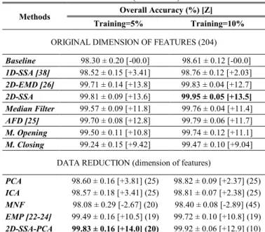
Finally, to further assess and validate the efficacy of the proposed 2D-SSA approach, additional results are included in Section V.D for comparison with other relevant methods. We divide these methods into two groups, the ones maintaining the original dimensionality of features, and the methods performing data reduction. Considering the difference in terms of parameter configurations, the best results obtained from median filtering, AFD, morphological opening and closing, and EMP are given. Classical techniques such as PCA, ICA, and MNF are also included along with a fusion of our spatial-domain 2D-SSA with spectral domain 1D-PCA (2D-SSA-PCA) for exploiting spatial-spectral feature extraction in the hypercube.
D. Data Classification
Exploiting a margin-based criterion, SVM appears to be very robust to potential problems such as the Hughes phenomenon [8]. With better results produced over other classifiers, SVM has been widely used in HSI field [5-7, 26]. In addition, there are several available libraries supporting multiple functions of SVM, which makes it easy to implement even in embedded systems [55-56]. According to all this, SVM is selected as a classifier. For multi-class classification, LibSVM library [57] is used in our experiments for supervised learning, allowing fast and accurate data modeling.
SVM supports different types of kernel functions including linear, polynomial and Gaussian radial basis function. Each kernel offers a proper performance depending on the data to evaluate. From our own experience but also suggested by others [5-7, 26], the Gaussian kernel usually performs well in HSI classification. Consequently, Gaussian kernel is used in our experiments, where the penalty c and the gamma parameters are tuned every time through a grid search procedure.
Additionally, to further validate the efficacy of our proposed approach, a classical k-nearest neighbor (k-NN) classifier [58], using parameter k=3, is implemented for the 92AV3C data set. As k-NN is a weaker classifier than SVM, a potential improvement in classification accuracy will show the effectiveness of 2D-SSA features, regardless the classifiers employed.
In order to provide statistical significance and avoid systematic errors, each experiment is repeated ten times with different training and testing subsets. In each of the ten repetitions, which are common for all the methods evaluated, training and testing partitions are randomly obtained, with no sample overlap allowed. Through stratified sampling an equal sample rate of 10% was used for each class in the training process. Same experiments with a rate of 5% for training are also reported for comparison.
Results from the testing samples classification are provided by the mean value and standard deviation over the ten repetitions, expressed in terms of overall accuracy, although extra evaluations based on average accuracy and class-by-class accuracy are also provided for some experiments. In addition, McNemar’s test [59] is used as a complementary measurement of classification accuracy performance. This test is based on the standardized normal test statistic, and having the Baseline approach as a reference,
the sign of the parameter Z denotes if the method evaluated outperforms the reference (positive Z), expressing proper statistical significance at a confidence level of 95% when Z > 1.96. Comprehensive results with analysis are presented and evaluated in the next section.
V. RESULTS AND EVALUATIONS
Using the three data sets and the experimental setup discussed in the previous section, comprehensive experiments have been carried out for performance evaluation. At this aim, the present section is divided in fiveparts described as follows.
First, according to the experimental settings in Table I, results from 2D-SSA method are compared with Baseline reference, 1D-SSA and 2D-EMD. The comparisons are made on the basis of the overall accuracy classification with McNemar’s test [59], where for each experiment the mean value and the standard deviation along ten repetitions are used to show statistical significance. In addition, the class-by-class and average accuracies are also shown in some cases providing further assessment.
Second, the execution time required in 2D-EMD and 2D-SSA for feature extraction under different parameter values is confronted to clearly show the advantge of our proposal with respect to 2D-EMD.
Then, the effect of parameter selection in the 2D-SSA method is evaluated to address the appropriate parameter tuning in the implementation and also to justify the general behavior of the proposed 2D-SSA approach for feature extraction.
Afterwards, the 2D-SSA method is further compared to several other state-of-the-art techniques, including its extended version 2D-SSA-PCA. These experiments are implemented under the same experimental settings used previously, where the best performance for each method is reported for comparison.
Finally, the proposed 2D-SSA method working with a relative weak classifier (k-NN) rather than SVM is further evaluated. This is to prove the added value of our proposal in feature extraction terms, as it can effectively work with different classifiers. Relevant results and analysis are reported in detail below.
A. Classification Accuracy Comparison
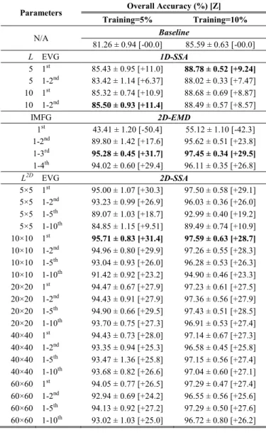
For the three data sets 92AV3C, Pavia UA and Salinas C, results under various experimental conditions with different parameters values are given in Table II, Table III, and Table IV, respectively, including McNemar’s test of significance.
With 2D-SSA, consistently significant improvements are achieved for all the three data sets compared to the Baseline approach and the 1D-SSA method, due to the spatial structures preserved and noise removed. In the first data set (Table II), the classification accuracy has increased from 81.3% and 85.6% to over 95.7% and 97.6%, under a training ratio of 5% and 10%, respectively. In the other two data sets, the best accuracy achieved by 2D-SSA is near 100%. In comparison to 2D-EMD, 2D-SSA yields comparable or slightly better results, achieving impressive results in relation to the Baseline case and the 1D-SSA approach.
It is worth noting that the 2D-EMD method is highly dependent on the number of IMFs used for the reconstruction of signal. Indeed, using the first IMF for reconstruction usually leads to deterioration in the accuracy compared to the Baseline, whilst 2D-SSA always shows a much more reliable and consistent behavior under different implementation conditions.
TABLEII
MEAN OVERALL ACCURACY (%)OVER TEN REPETITIONS WITH STANDARD DEVIATION AND MEAN MCNEMAR’S TEST [Z] FOR THE 92AV3CDATA SET BY
DIFFERENT METHODS AND PARAMETERS FOR FEATURE EXTRACTION
Parameters Overall Accuracy (%) [Z] Training=5% Training=10% N/A Baseline 81.26 ± 0.94 [-00.0] 85.59 ± 0.63 [-00.0] L EVG 1D-SSA 5 1st 85.43 ± 0.95 [+11.0] 88.78 ± 0.52 [+9.24] 5 1-2nd 83.42 ± 1.14 [+6.37] 88.02 ± 0.33 [+7.47] 10 1st 85.32 ± 0.74 [+10.9] 88.68 ± 0.69 [+8.87] 10 1-2nd 85.50 ± 0.93 [+11.4] 88.49 ± 0.57 [+8.57] IMFG 2D-EMD 1st 43.41 ± 1.20 [-50.4] 55.12 ± 1.10 [-42.3] 1-2nd 89.80 ± 1.42 [+17.6] 95.62 ± 0.51 [+23.8] 1-3rd 95.28 ± 0.45 [+31.7] 97.45 ± 0.34 [+29.5] 1-4th 94.02 ± 0.60 [+29.4] 96.11 ± 0.35 [+26.8] L2D EVG 2D-SSA 5×5 1st 95.00 ± 1.07 [+30.3] 97.50 ± 0.58 [+29.1] 5×5 1-2nd 93.23 ± 0.99 [+26.9] 96.03 ± 0.36 [+26.0] 5×5 1-5th 89.07 ± 1.03 [+18.7] 92.99 ± 0.40 [+19.2] 5×5 1-10th 84.85 ± 1.15 [+9.51] 89.49 ± 0.74 [+10.9] 10×10 1st 95.71 ± 0.83 [+31.4] 97.59 ± 0.63 [+28.7] 10×10 1-2nd 94.96 ± 0.80 [+29.9] 97.26 ± 0.55 [+28.3] 10×10 1-5th 93.04 ± 0.93 [+26.0] 96.28 ± 0.53 [+26.3] 10×10 1-10th 91.42 ± 0.92 [+23.2] 94.90 ± 0.46 [+23.3] 20×20 1st 94.47 ± 0.67 [+27.9] 97.23 ± 0.61 [+27.5] 20×20 1-2nd 94.43 ± 0.91 [+27.9] 97.36 ± 0.56 [+27.9] 20×20 1-5th 94.90 ± 0.66 [+29.5] 97.43 ± 0.51 [+28.5] 20×20 1-10th 93.70 ± 0.75 [+27.3] 96.91 ± 0.53 [+27.4] 40×40 1st 94.43 ± 0.73 [+28.0] 97.14 ± 0.67 [+27.3] 40×40 1-2nd 93.35 ± 0.94 [+25.3] 96.58 ± 0.45 [+25.8] 40×40 1-5th 93.47 ± 1.36 [+25.8] 97.15 ± 0.56 [+27.4] 40×40 1-10th 93.68 ± 0.82 [+26.6] 97.04 ± 0.60 [+27.1] 60×60 1st 94.05 ± 0.77 [+26.5] 97.29 ± 0.47 [+27.4] 60×60 1-2nd 92.94 ± 0.69 [+24.2] 96.55 ± 0.56 [+25.6] 60×60 1-5th 94.13 ± 0.92 [+27.2] 97.29 ± 0.50 [+27.6] 60×60 1-10th 93.02 ± 1.03 [+25.0] 96.72 ± 0.80 [+26.2] TABLEIII
MEAN OVERALL ACCURACY (%)OVER TEN REPETITIONS WITH STANDARD DEVIATION AND MEAN MCNEMAR’S TEST [Z] FOR THE PAVIA UADATA SET BY
DIFFERENT METHODS AND PARAMETERS FOR FEATURE EXTRACTION
Parameters Overall Accuracy (%) [Z] Training=5% Training=10% N/A Baseline 95.83 ± 0.79 [-00.0] 96.67 ± 0.32 [-00.0] L EVG 1D-SSA 5 1st 95.37 ± 0.86 [-2.44] 96.50 ± 0.31 [-0.88] 5 1-2nd 95.53 ± 0.72 [-1.88] 96.60 ± 0.36 [-0.69] 10 1st 95.21 ± 0.55 [-3.12] 96.15 ± 0.35 [-2.47] 10 1-2nd 95.00 ± 0.84 [-4.14] 96.30 ± 0.52 [-2.12]
IMFG 2D-EMD 1st 69.50 ± 1.75 [-38.1] 77.72 ± 1.63 [-30.8] 1-2nd 94.36 ± 0.73 [-4.16] 97.52 ± 0.34 [+2.92] 1-3rd 98.92 ± 0.34 [+11.6] 99.67 ± 0.11 [+12.5] 1-4th 99.53 ± 0.31 [+14.6] 99.80 ± 0.08 [+13.5] L2D EVG 2D-SSA 5×5 1st 97.97 ± 0.38 [+7.31] 99.18 ± 0.28 [+9.92] 5×5 1-2nd 98.21 ± 0.35 [+8.55] 98.99 ± 0.31 [+9.44] 5×5 1-5th 97.57 ± 0.59 [+6.63] 98.90 ± 0.26 [+9.58] 5×5 1-10th 97.21 ± 0.66 [+5.85] 98.18 ± 0.34 [+6.84] 10×10 1st 97.77 ± 0.45 [+6.23] 98.92 ± 0.28 [+8.54] 10×10 1-2nd 96.96 ± 0.64 [+3.56] 98.36 ± 0.39 [+6.20] 10×10 1-5th 97.38 ± 0.64 [+5.19] 98.89 ± 0.44 [+8.76] 10×10 1-10th 97.94 ± 0.44 [+7.59] 98.86 ± 0.29 [+9.02] 20×20 1st 96.03 ± 0.75 [+0.56] 97.47 ± 0.47 [+2.64] 20×20 1-2nd 97.07 ± 0.65 [+3.78] 98.43 ± 0.37 [+6.24] 20×20 1-5th 97.20 ± 0.23 [+4.27] 98.51 ± 0.39 [+6.79] 20×20 1-10th 96.67 ± 1.27 [+2.86] 98.76 ± 0.30 [+8.03] 40×40 1st 95.91 ± 0.89 [+0.24] 97.64 ± 0.35 [+3.16] 40×40 1-2nd 96.38 ± 1.04 [+1.68] 98.32 ± 0.53 [+5.87] 40×40 1-5th 96.99 ± 0.40 [+3.54] 98.06 ± 0.42 [+4.92] 40×40 1-10th 96.42 ± 0.65 [+1.74] 97.80 ± 0.45 [+3.94] 60×60 1st 96.69 ± 0.42 [+2.46] 97.86 ± 0.45 [+4.02] 60×60 1-2nd 96.38 ± 0.44 [+1.60] 98.23 ± 0.33 [+5.48] 60×60 1-5th 96.35 ± 0.89 [+1.64] 97.98 ± 0.35 [+4.55] 60×60 1-10th 96.78 ± 0.70 [+2.96] 98.08 ± 0.55 [+5.09] TABLEIV
MEAN OVERALL ACCURACY (%)OVER TEN REPETITIONS WITH STANDARD DEVIATION AND MEAN MCNEMAR’S TEST [Z] FOR THE SALINAS CDATA SET BY
DIFFERENT METHODS AND PARAMETERS FOR FEATURE EXTRACTION
Parameters Overall Accuracy (%) [Z] Training=5% Training=10% N/A Baseline 98.30 ± 0.20 [-00.0] 98.61 ± 0.12 [-00.0] L EVG 1D-SSA 5 1st 98.46 ± 0.22 [+2.47] 98.76 ± 0.12 [+2.03] 5 1-2nd 98.52 ± 0.15 [+3.41] 98.69 ± 0.09 [+1.21] 10 1st 98.39 ± 0.28 [+1.66] 98.68 ± 0.09 [+0.78] 10 1-2nd 98.42 ± 0.22 [+1.33] 98.76 ± 0.14 [+2.00] IMFG 2D-EMD 1st 68.58 ± 0.85 [-65.3] 76.42 ± 0.64 [-54.3] 1-2nd 94.56 ± 0.55 [-18.5] 97.56 ± 0.27 [-6.92] 1-3rd 99.54 ± 0.17 [+12.2] 99.78 ± 0.05 [+12.2] 1-4th 99.71 ± 0.14 [+13.8] 99.83 ± 0.04 [+12.7] L2D EVG 2D-SSA 5×5 1st 99.51 ± 0.17 [+10.6] 99.77 ± 0.06 [+11.1] 5×5 1-2nd 99.32 ± 0.13 [+9.45] 99.68 ± 0.07 [+10.3] 5×5 1-5th 98.94 ± 0.19 [+6.33] 99.31 ± 0.18 [+7.35] 5×5 1-10th 98.63 ± 0.12 [+4.01] 98.93 ± 0.18 [+3.64] 10×10 1st 99.58 ± 0.26 [+11.2] 99.74 ± 0.12 [+10.8] 10×10 1-2nd 99.34 ± 0.23 [+8.79] 99.69 ± 0.13 [+10.2] 10×10 1-5th 99.44 ± 0.19 [+10.3] 99.77 ± 0.06 [+11.4] 10×10 1-10th 99.06 ± 0.17 [+7.35] 99.47 ± 0.23 [+8.85] 20×20 1st 99.62 ± 0.12 [+11.3] 99.81 ± 0.12 [+11.3] 20×20 1-2nd 99.34 ± 0.15 [+8.55] 99.77 ± 0.12 [+11.0] 20×20 1-5th 99.50 ± 0.24 [+10.5] 99.79 ± 0.08 [+11.3] 20×20 1-10th 99.35 ± 0.13 [+9.17] 99.75 ± 0.05 [+10.9] 40×40 1st 99.67 ± 0.17 [+12.0] 99.85 ± 0.08 [+12.1] 40×40 1-2nd 99.81 ± 0.09 [+13.6] 99.93 ± 0.05 [+13.1]
40×40 1-5th 99.46 ± 0.24 [+9.88] 99.81 ± 0.08 [+11.6] 40×40 1-10th 99.56 ± 0.13 [+11.0] 99.77 ± 0.09 [+11.1] 60×60 1st 99.63 ± 0.15 [+11.9] 99.90 ± 0.11 [+12.8] 60×60 1-2nd 99.75 ± 0.15 [+13.0] 99.95 ± 0.05 [+13.5] 60×60 1-5th 99.65 ± 0.20 [+12.1] 99.92 ± 0.05 [+13.0] 60×60 1-10th 99.58 ± 0.17 [+11.1] 99.77 ± 0.07 [+11.1] TABLEV
MEAN OVERALL,AVERAGE AND CLASS-BY-CLASS ACCURACY VALUES (%) OVER TEN REPETITIONS FOR THE 92AV3CDATA SET WITH BASELINE,1D-SSA(L=5, EVG=1ST
),2D-EMD(IMFG=1-3RD
), AND 2D-SSA(L=10,EVG=1ST
)METHODS USING TRAINING=10%,INCLUDING NUMBER OF SAMPLES (NOS)
NoS Baseline 1D-SSA 2D-EMD 2D-SSA
Class 1 1434 80.71 84.81 95.53 96.35 Class 2 834 72.03 80.99 95.96 97.72 Class 3 497 89.98 92.73 96.38 96.76 Class 4 747 97.23 97.77 99.36 97.92 Class 5 489 99.00 99.11 99.45 99.18 Class 6 968 76.83 83.54 94.73 95.74 Class 7 2468 83.99 86.11 98.48 98.27 Class 8 614 80.45 84.91 95.89 95.94 Class 9 1294 98.27 98.41 99.90 99.27 Average Accuracy 86.50 89.82 97.30 97.46 Overall Accuracy 85.59 88.78 97.45 97.59 TABLEVI
MEAN OVERALL,AVERAGE AND CLASS-BY-CLASS ACCURACY VALUES (%) OVER TEN REPETITIONS FOR THE PAVIA UADATA SET WITH BASELINE,1D-SSA(L=5, EVG=1-2ND
),2D-EMD(IMFG=1-4TH
), AND 2D-SSA(L=5,EVG=1ST
)METHODS USING TRAINING=10% AND INCLUDING NUMBER OF SAMPLES (NOS)
NoS Baseline 1D-SSA 2D-EMD 2D-SSA
Class 1 310 81.94 81.72 99.86 96.70 Class 2 957 97.21 97.07 100 100 Class 3 154 96.23 96.30 99.28 94.49 Class 4 698 99.67 99.71 99.62 100 Class 5 2559 97.57 97.42 99.89 99.79 Class 6 860 95.27 95.44 99.85 98.46 Class 7 854 96.63 96.51 99.48 98.54 Class 8 293 100 100 99.77 98.17 Average Accuracy 95.56 95.52 99.72 98.27 Overall Accuracy 96.67 96.60 99.80 99.18 TABLEVII
MEAN OVERALL,AVERAGE AND CLASS-BY-CLASS ACCURACY VALUES (%) OVER TEN REPETITIONS FOR THE SALINAS CDATA SET WITH BASELINE,1D-SSA(L=5, EVG=1ST
),2D-EMD(IMFG=1-4TH
), AND 2D-SSA(L=60,EVG=1-2ND
)METHODS,USING TRAINING=10% AND INCLUDING NUMBER OF SAMPLES (NOS)
NoS Baseline 1D-SSA 2D-EMD 2D-SSA
Class 1 240 95.32 95.56 100 100 Class 2 3400 99.93 99.92 99.96 100 Class 3 1957 99.71 99.80 99.88 99.96 Class 4 599 99.13 98.42 99.09 99.70 Class 5 1155 97.77 98.40 98.78 99.95 Class 6 1414 99.99 99.99 99.98 100 Class 7 848 99.62 99.65 99.93 99.99 Class 8 5890 99.23 99.35 99.99 99.98 Class 9 159 25.52 32.59 98.81 97.97 Average Accuracy 90.69 91.52 99.60 99.73 Overall Accuracy 98.61 98.76 99.83 99.95
Not only the overall accuracy but also complementary class-by-class and average accuracies are employed to assess the classification results, as shown in Table V-VII. For the three data sets, the best results achieved in each method under a training rate of 10% are compared. As can be seen, similar to the 2D-EMD case, the increment in classification accuracy for 2D-SSA is generally achieved in every labeled class, independently from the corresponding number of samples. This has clearly proved that 2D-SSA method can achieve similar (or even better) performance as 2D-EMD in terms of classification accuracy.
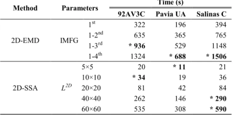
B. Running Time Comparison between 2D-EMD and 2D-SSA
Although the results from 2D-EMD are similar to those from 2D-SSA, the execution times required for feature extraction, as compared in Table VIII, are much different. For 2D-EMD, feature extraction using the parameters with good classification accuracy needs 936, 688 and even 1506 seconds for the 92AV3C, Pavia UA, and Salinas C data sets, respectively. 2D-SSA, for similar results, can reduce massively this timing to only few seconds, one and even two orders of magnitude less. The reason behind is that 2D-SSA has a straight implementation based on the well-known SVD (or equivalent EVD), which avoids empirical iterations as used in the 2D-EMD implementation. As a result, 2D-SSA allows faster data processing and makes the proposed approach more suitable for real-time applications.
TABLEVIII
APPROXIMATED EXECUTION TIME REQUIRED FOR 2D-EMD AND 2D-SSAFEATURE EXTRACTION INDICATING THE BEST CASE (*) IN TERMS OF MEAN OVERALL
ACCURACY CLASSIFICATION
Method Parameters Time (s)
92AV3C Pavia UA Salinas C
2D-EMD IMFG 1st 322 196 394 1-2nd 635 365 765 1-3rd * 936 529 1148 1-4th 1324 * 688 * 1506 2D-SSA L2D 5×5 20 * 11 21 10×10 * 34 19 36 20×20 81 42 84 40×40 262 146 * 290 60×60 535 308 * 590
C. Evaluation on 2D-SSA Parameters Selection
Though it is clear that 2D-SSA is useful in improving the classification accuracy by effective feature extraction in the spatial domain whilst suppressing the effect of noise, its performance is parameter dependent. As stated in Golyandina et al [36], the properties of the data set affect the results and behavior and this explains why the parameters need to be properly tuned.
In our group of experiments, the window size varies from 5×5, 10×10, 20×20, 40×40 to 60×60 and the number of Eigenvalue components used for grouping changes among the first, the first two, the first five, and the first ten. Most combinations of window size L2D=Lx×Ly and EV groupings generates great performance in classification accuracy terms, all of them clearly improving the efficacy achieved by the Baseline and 1D-SSA methods. Though many different values are used for the parameters, similar results are always obtained to show the reliability and constant behavior of 2D-SSA. According to the results shown in Tables II-IV, in
general only combinations of small L2D with large EVG may lead to less increment in the accuracy, although always above the Baseline reference. This is because as long as more of the extracted components are included in the grouping, the reconstruction is closer to the original image, being finally equivalent to it if all components are selected. Therefore, the main point is to avoid the combination of large EVG covering much of the Eigenvalue range offered by a given window L2D.
Regarding the performance in execution time terms, the use of large windows introduces more complexity in the 2D-SSA implementation, due to the matrix Sin the SVD, sized L2D×L2D, that is much larger and leads to increased execution times. As can be seen, time needed in the 2D-SSA feature extraction increases exponentially along with the window size. Nevertheless, slowest time in these cases is still about half the time needed by 2D-EMD feature extraction, for respective data sets. This fact makes definitely preferable the use of small windows, which confirms the general recommendation of going for small windows and small EVG selection in the implementation of 2D-SSA, at least when SVM is used as the classifier.
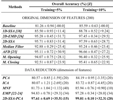
D. Comparison with other state-of-the-art techniques
To further validate the efficacy of the proposed 2D-SSA approach, several other state-of-the-art approaches, divided in two groups, are used for performance assessment. In the first group of approaches, the dimension of the feature remains the same, where 2D-SSA is compared with median filtering, AFD, morphological opening and closing as well as 1D-SSA, 2D-EMD and the Baseline. In the second group, dimension reduction is comprised after feature extraction. These include classical approaches such as PCA, ICA and MNF as well as EMP and 2D-SSA-PCA. Relevant results are reported in Tables IX-XI for detailed comparison. Actually, the excellent performance from 2D-SSA-PCA has demonstrated the great potential to combine 2D-SSA with other techniques in the process flow of HSI for future investigations.
In Tables IX-XI, for each method its best result achieved from several different parameter configurations are given for comparison. For the Baseline, 1D-SSA [38], 2D-EMD [26] and 2D-SSA, the complete configurations and results can also be found in Section V. The size of the median filter varies from 3x3, 5x5, 7x7, 9x9 to 11x11 [25]. For the AFD method, we implement it with different number of bins (from 2 to 6), where the corresponding sizes are 1x1, 3x3, 5x5, 7x7, 9x9, and 11x11 [25]. The morphological openings and closings use a disk as a structural element, with a radio size of 2, 4, 6, 8, and 10 [22-24]. For the classical PCA, ICA and MNF, the number of resulting features within 5 to 50 is tested [20]. For the EMP approach we use 1-3 components with openings/closings and radius increments as suggested in [22-24]. Finally, for