Supervised fault detection using unstructured server-log data to support root cause analysis

(1)

ZAHRA ABBASZADEH

SUPERVISED FAULT DETECTION USING UNSTRUCTURED

SERVER-LOG DATA TO SUPPORT ROOT CAUSE ANALYSIS

Master of Science thesis

Examiner: Prof. Moncef Gabbouj, Prof. Mikko Valkama

Examiner and topic approved by the Faculty Council of the Faculty of Computing and Electrical Engineer-ing on 5th November 2014

(2)

ABSTRACT

TAMPERE UNIVERSITY OF TECHNOLOGY

Master’s Degree Programme in Information Technology

ZAHRA ABBASZADEH: Supervised Fault Detection Using Unstructured Serv-er-Log Data to Support Root Cause Analysis

Master of Science Thesis, 48 pages November 2014

Major: Wireless Communication Circuits and Systems Examiner: Prof. Moncef Gabbouj, Prof. Mikko Valkama

Keywords: fault detection, supervised learning, linear classification, SVM, log data

Fault detection is one of the most important aspects of telecommunication networks. Considering the growing scale and complexity of communication networks, mainte-nance and debugging have become extremely complicated and expensive. In complex systems, a higher rate of failure, due to the large number of components, has increased the importance of both fault detection and root cause analysis. Fault detection for munication networks is based on analyzing system logs from servers or different com-ponents in a network in order to determine if there is any unusual activity. However, detecting and diagnosing problems in such huge systems are challenging tasks for hu-man, since the amount of information, which needs to be processed goes far beyond the level that can be handled manually. Therefore, there is an immense demand for auto-matic processing of datasets to extract the relevant data needed for detecting anomalies. In a Big Data world, using machine learning techniques to analyze log data automatical-ly becomes more and more popular. Machine learning based fault detection does not require any prior knowledge about the types of problems and does not rely on explicit programming (such as rule-based). Machine learning has the ability to improve its per-formance automatically through learning from experience.

In this thesis, we investigate supervised machine learning approaches to detect known faults from unstructured log data as a fast and efficient approach. As the aim is to identi-fy abnormal cases against normal ones, anomaly detection is considered to be a binary classification. For extracting numerical features from event logs as a primary step in any

(3)

classification, we used windowing along with bag-of-words approaches considering their textual characteristics (high dimension and sparseness).

We focus on linear classification methods such as single layer perceptron and Support Vector Machines as promising candidate methods for supervised fault detection based on the textual characteristics of network-based server-log data. In order to generate an appropriate approach generalizing for detecting known faults, two important factors are investigated, namely the size of datasets and the time duration of faults. By investigat-ing the experimental results concerninvestigat-ing these two aforementioned factors, a two-layer classification is proposed to overcome the windowing and feature extraction challenges for long lasting faults. The thesis proposes a novel approach for collecting feature vec-tors for two layers of a two-layer classification. In the first layer we attempt to detect the starting line of each fault repetition as well as the fault duration. The obtained mod-els from the first layer are used to create feature vectors for the second layer. In order to evaluate the learning algorithms and select the best detection model, cross validation and F-scores are used in this thesis because traditional metrics such as accuracy and error rates are not well suited for imbalanced datasets.

The experimental results show that the proposed SVM classifier provides the best per-formance independent of fault duration, while factors such as labelling rule and reduc-tion of the feature space have no significant effect on the performance. In addireduc-tion, the results show that the two-layer classification system can improve the performance of fault detection; however, a more suited approach for collecting feature vectors with smaller time span .needs to be further investigated.

(4)

PREFACE

This work has been conducted at the Department of Signal Processing of Tampere Uni-versity of Technology in collaboration with TIETO within ICT SHOK D2I project.. I would like to express my deepest gratitude to my supervisor Prof. Moncef Gabbouj who trusted me in the first place giving me the opportunity to work in his research group while fully helping me throughout this process. This thesis could not be accom-plished without his support.

I would like to thank Professor Mikko Valkama especially for revising my thesis and acting as an examiner.

My big appreciation goes to my co-supervisors Honglei Zhang and Dr. Stefan Uhlmann. Honglei supported and guided me throughout my research while Stefan provided me with constructive comments while writing the thesis. This thesis owes its existence to Stefan’s great efforts, patience and feedback.

I would also like to thank my collaborators from Tieto, especially Harri Kukkasniemi, for providing me with the required dataset and helping me to conduct the research smoothly.

I do not have enough words to thank Sharareh Naghdi who has acted like my dearest sister and has made my life abroad memorable.

I would like to specially mention my friend Dr. Payman Aflaki for his help and sugges-tions on how to write this thesis.

Last but not least, my sincere gratitude goes my husband, Mehrdad, who experienced all ups and downs of my research. Moreover, I dedicate this thesis to my parents for their endless support and encouragement.

(5)

LIST OF FIGURES

Figure 2. 1 The sign of the projection onto the weight vector W yields the class

label………...10

Figure 2. 2 Finding the best separating hyper-plane………...11

Figure 2. 3 Margin and support vectors for SVMS………...…...11

Figure 3. 1. Overview of the learning algorithm………...……17

Figure 3. 2. A part of ground truth dataset, fault logs labelled as 1 and normal logs labelled as 0………...……18

Figure 3. 3. Sequence of logs and their corresponding tokens………..…....19

Figure 3. 4. Assign label to each feature vector………....…20

Figure 3. 5. Sliding window to collect feature vector………..21

Figure 3. 6. Feature extraction approach of first layer………..………24

Figure 3. 7. Creating first feature vector of second layer………...……..…....25

Figure 3. 8. Creating second feature vector for second layer………26

Figure 3. 9. Feature vector consists of last five values from start-predicted-model and statistical values from middle-predicted-model……….…27

Figure 3. 10. After detection of fault logs, only the last four elements of feature vector will be changed………....……28

Figure 3. 11. By ending the fault logs and indicating normal logs both buffer and mid-dle-prob-estimate reset and procedure starts from first step………..………29

Figure4. 1. A part of Fault List Log illustrating two different faults, and time duration of each repetition……….….…………31

Figure4. 2. Confusion Matrix……….…….………33

Figure 4. 3. Performance of different classifiers……….……….……35

Figure 4. 4. Comparison bag-of-words vs bag-of-strings……….………….…36

(7)

Figure 4. 6. Performance of two layer classification vs one layer classification………38 Figure 4. 7. The results of LIBLINEAR on fault 1 with duration between 12 minutes to 22 minutes for different window sizes………...……39 Figure 4. 8. The results of LIBLINEAR on fault 3 with duration around 4:30 minutes for different window sizes………...……39 Figure 4. 9. The results of LIBLINEAR on fault 4 with duration around 8 seconds for different window sizes……….….……40 Figure 4. 10. The results of LIBLINEAR on fault 5 with duration around 2 minutes for different window sizes ……….………...……40

(8)

LIST OF SYMBOLS AND ABBREVIATIONS

3G Third generation of mobile telecommunications technology 4G Fourth generation of mobile telecommunications technology

BCCH Broadcast Control CHannel

FN False Negative

FP False Positive

FV1 Feature vector correspond to first window FV1-L2 First feature vector of second layer

HDD Hard Disk Drive

LTE Long-Term Evolution

SVM Support Vector Machine

LIBSVM An implementation of Support Vector Machine LIBLINEAR An implementation of linear regression

TC Text Classification

TF Term Frequency

TF-IDF Term Frequency-Inverse Document Frequency

TTY Unstructured log data including two days of network traffic data with one fault type

TTY-2 Unstructured log data including five days of network traffic data with five fault types

TP True Positive

TN True Negative

(9)

(10)

1.

INTRODUCTION

Wireless communication is one of the big engineering success stories of recent years – not only from a scientiﬁc point of view, where the progress has been astonishing but also with respect to market size and impact on society. Cellular telephony is big evi-dence, as it is the biggest market segment, and has the highest impact on everyday lives. The popularity of mobile devices grows, as their offered capabilities and services increase. The growing scale of services they offer, diversity of devices connected to the network, introducing Heterogeneous Networks combining different Radio Access Technologies (3G, LTE (Long-Term Evolution), Wi-Fi (Wireless fidelity)) and more recently, variety of network topologies they can use, cause mobile communication net-works to become more complex distributed systems ‎[9]. High level of distributions results in producing huge amounts of data including, for example, measurements indi-cating radio interface efficiency and log data from different components ‎[50].

As wireless systems are being increasingly used, it is becoming a challenge to debug and keep network operation stable, fault free, and secure. In complex systems, a higher rate of failure, due to the large number of components, has increased the importance of both fault detection and root cause analysis. Such failures can be caused by different sources such as power break down, hardware failure, software bugs, wrong configura-tions, human mistakes, and intrusive attacks. Root cause of a failure is the reason for which it occurs and root cause analysis is based on detecting and fixing the problem and preventing it from reoccurring.

The logs generated by network systems are generally time-series data streams con-tained messages that represent the status of a running system and other expansive in-formation to support fault diagnosis. Therefore, syslog analysis plays an essential role for detecting failures in large systems ‎[1]. However analyzing system logs manually is not realistic and practical since in a complex system various parts produce huge amounts of logs every day, which not all of them are interesting for error detection. Furthermore, software and hardware are developed and updated frequently leading to a considerable change of log files. As there is no standard structure for all log files, it is

(11)

infeasible to utilize a unique single log analyzer for a developing large system. Moreo-ver, training many people to be as familiar with all system details is costly and time consuming ‎[62]. To cope with these issues, machine learning techniques are introduced and exploited to automate the process of log analysis. Machine learning techniques can automatically process large scale data and improve their performance through learning patterns on a set of training data and then apply to new unknown data. In the field of intrusion detection, the advantages of machine learning techniques are their ability to detect unexpected problems and analyze all logs much faster than humans. Machine learning techniques do not rely on explicit programming. In addition, the developer of a machine learning system does not need to have any expert knowledge in log analysis; however, it could be helpful to find high quality features.

In this thesis, we investigate supervised machine learning approaches to detect known faults from unstructured log data simulated and provided by TIETO since these learn-ing methods are fast and powerful in detectlearn-ing known network faults and problems. Generally, supervised machine learning techniques make use of pre-existing knowledge and are first trained to generate models by using characteristics of labeled training data. Then the models are applied to identify faults and/or intrusions in unseen test data. But the preliminary and most important step in machine learning based fault detection sys-tems is to extract numerical informative features from dataset since the performance of classification tasks is affected by representation of features.

To select appropriate feature extraction and classification methods, we focus on stream-ing and textual characteristics of log data as available dataset in communication net-works. The used approach for feature extraction and collecting feature vectors in this thesis is sliding window (considering streaming characteristics of data) along with bag-of-words (considering textual characteristics of data). Regarding the textual characteris-tics of log data, linear classification techniques are proposed for learning algorithm. From various linear classification techniques, we choose to investigate two methods of single layer perceptron and Support Vector Machines (SVMs) with more focus on SVMs. Since SVMs are one of the best learning algorithms for binary classification that is relevant in this thesis to detect abnormal logs against normal ones ‎[50‎, 83 and 1]. There are different implementations of SVMs. In this thesis, we compare the results of LIBLINEAR versus LIBSVM.

(12)

Our experiments are established in two phases based on usage of two different datasets. We explore the effects of using bag-of-strings instead of bag-of-words for feature ex-traction in order to reduce the dimension of feature space and different rules for label-ling the feature vectors. The most challenging task in this thesis is to deal with long lasting faults. From classification point of view long lasting fault means that one class dominants the entire dataset while there is rare occurrences of another class. The prob-lem with these kinds of dataset is low quality of their performance using standard de-tection approaches. To address this problem, this thesis proposes a two-layer classifica-tion with novel approaches for collecting feature vectors of each layer. The results show high performance of two-layer classification in compare to one layer classifica-tion for long fault duraclassifica-tions. However, creating feature vectors for two layers are more time consuming. The rest of this thesis is organized as follows.

Chapter 2 provides background information and highlights the research relevant to this thesis. In this chapter, first the common approaches to extract features from text data and streaming data and previous work on feature extraction of log data are reviewed in general. Then the used classification methods in this thesis are introduced. In addition, two major detection approaches and various methods of intrusion detection used by researchers are given in this chapter.

Chapter 3 presents an overview of our approach for feature extraction, creating feature vectors and learning algorithm.

Chapter 4 introduces evaluation metrics and represents the experiments and results. In this chapter various factors that may affect the results are compared and the results of the chosen classification methods are illustrated.

Chapter 5 concludes and discusses limitations of supervised classification over unstruc-tured network log-data.

(13)

2.

BACKGROUND

Mobile networks have become interesting and popular networks in recent years due to the rapid increasing of wireless devices such as mobile laptop computers, PDAs and wireless telephones and growing scale of services they offer. As mobile networks be-come more popular and widely used, their operation, maintenance, security and in gen-eral, protecting them against anomalous network behavior to improve services and support this popularity, has become one of the major concerns. The anomalies can be defined as a data pattern, which is different from normal data and requires atten-tion ‎[74]. Consequently, detecting anomalous behavior is an indispensable task in net-work operation. Anomaly detection for communication netnet-works is based on analyzing system logs from servers or different components in a network and determines whether there is any unusual activity. However, detecting and diagnosing problems in such huge systems is a challenging task for both developers and operators since the amount of information needed to process them goes far beyond the level that can be handled man-ually ‎[83]. Therefore, there is an immense demand for automatic processing of datasets to extract the relevant data needed for detecting anomalies.

Generally, datasets in communication networks are represented in log format. The log format varies by types of components that generate it. The only parts of each log to correlate various types of unstructured log data are timestamps. Therefore, logs estab-lish unstructured time series files, and event logs are non-numerical logs in which the messages contain vocabulary of terms (or phrases). In this thesis, the datasets to ana-lyze are event logs and by terms of system log or syslog I mean event logs. Thus, to analyze the log files and collect feature vectors to apply machine learning techniques and detect the anomalies, we consider approaches used for both textual data and streaming data.

In this chapter, we first review feature extraction methods for text data and online streaming data. Then we look at text classification focusing on linear classification, as a

(14)

main approach applied to event logs. The last part of this chapter reviews previous anomaly detection methods for log data.

2.1

Feature extraction

Feature extraction is a core and preliminary step of any classification using machine learning techniques. Considering aforementioned characteristics of event logs, we need to combine the feature extraction methods of streaming data with textual feature extrac-tion methods. In following a brief overview of feature extracextrac-tion methods for both tex-tual data and streaming data is represented., and then some researches on extracting features and mining the patterns of logs which could be used in machine learning tech-niques are reviewed.

2.1.1

Feature extraction methods for text documents

In text analysis such as natural language document classification, the main idea for fea-ture extraction is to extract words from the raw text data and convert them into numeri-cal features numeri-called term-based method, which gives a machine learning model a simpler and more focused view of the text. The most common way to address this issue is bag-of-words representation, which extracts numerical features from text content [1, 65]. In this technique, text data is considered to be a collection of words, and a dictionary is built by collecting all terms that occur at least once in a collection of documents. bag-of-words is a vector whose components represent the number of occurrence of each word in a document called term frequency (TF) while disregarding the position infor-mation of the words in the document. Normalization is applied to scale the term fre-quencies to values between 0 and 1 in order to measure the importance of a term in a document. In this scheme each individual components of term frequency vector or term weights vector is regarded as a feature ‎[65].

Besides words, using phrases rather than words referred as n-grams may also be used ‎[58] since a collection of words (unigrams) ignore any word order dependence and cannot consider phrases and multi-word expressions. Thus, in some cases, a collection of bigrams (n=2) or n-grams instead of unigrams is preferred, where occurrence of pairs or more consecutive words are counted ‎[65].

(15)

TF-IDF (Term Frequency-Inverse Document Frequency) is also a commonly used fea-ture in natural language processing (NLP) ‎[40]. By using this method, the weight of terms that occur frequently in a document is low and the weight of rarely occurrence increases in order to improve the accuracy of classification ‎[62‎, 56].

Feature selection is also an important issue in different classification methods, which is defined as selecting a subset of features from original features in order to reduce the dimension of text features and remove non-informative words from text data to im-prove learning performance ‎[79].

The most common and effective feature selection method in text data is stop-word re-moval [8‎, 18]. In ‎[84] a wide variety of feature selection methods in text categorization are compared and their experimental results discussed.

2.1.2

Feature extraction for online streaming data

A data stream is a massive real time sequence of data, which is continuous, ordered (by timestamp or arrival time), and fast changing. An issue concerning online streaming data processing is that to store an entire data stream or to scan through it several times is impossible due to its great volume. Sliding window approaches are a simple, widely used and standard way for feature extraction when dealing with streaming data. Moreo-ver, since data streams have a natural temporal ordering, new data are often more accu-rate and more relevant than older ones ‎[61].

For streaming (time-series) data processing, two types of sliding windows have been presented in different researches ‎[61, 27]. The main approach for both is to isolate the range of continuous data to a sliding window, either with a fixed size of window con-taining the most recent T items, called a count-base or a sequence-based sliding win-dow, or windows contain items from last t time units, called time-base or timestamp-based sliding window. Their performance is timestamp-based on making a window classifier that assign a label from predefined class labels or ground truth to each feature vector ex-tracted from input window of width w. Using this method, each sequence of data is segmented in temporal windows of fixed size of T items or time slices of t seconds in length defined as Li = < li,…,li+t-1> that starts at time i. Next temporal window is

(16)

by collecting features from each window and labeled them with a predefined categories based on defined decision rule. The reason for popularity of this method is its simplici-ty to apply to any classical learning algorithm.

2.1.3

Feature extraction for syslog data

Feature extraction for system logs is problem dependent and there is no generally ac-cepted standard in this area. For those kinds of logs contained numerical data, features are already provided that allows focusing on learning algorithm. But for time-series, meaningful non-numerical logs called event logs (indicating the state of systems), the features must be extracted since machine learning algorithm cannot process them di-rectly. Even though many different methods have been represented in various study researches ‎[83], this issue is still under investigation.

Considering the time-series characteristic of log files, sliding window methods have been widely used in many machine learning based anomaly detection techniques. ‎[83, 76, ‎74, ‎4, 9]. However, they used different methodology to extract features. For exam-ple in ‎[83], authors concentrate on two kinds of features, the state ratio vector using time-based window to analyze the behavior of the system over a certain period of time, and message count vector to collect problems concerning individual activities. Addi-tionally, they applied TF-IDF method to its message count vector in order to improve the accuracy of detecting errors of logs. Different researchers have used different meth-ods based on their applications. For example ‎[74] represent the frequencies of 2-grams as features for network logs. Authors in ‎[9] compare two one-class modelling tech-niques; one-class Support Vector Machines and a Hellinger distance-based one-class modeling in which the technique for extracting features is bag-of-words. Main concept on windowing combined with one of the feature extraction methods researches repre-sented tools to extract features from log files [‎83, 4]. They introduce either prepro-cessing technique ‎[83] or a tool to extract relative features more exactly ‎[4] to improve the detection results. In ‎[4] the semi unstructured time series database, Splunk, is repre-sented as a tool for automatic event boundary detection that breaks the text stream into separate events exploiting the timestamps. It is used to index, search, and analyze mas-sive datasets. The study ‎[83] used programming to extract structured information from unstructured data logs by parsing them and specifying their important properties.

(17)

Au-thors represent two kinds of properties, identifiers variables to identify the program object which can take a large number of distinct values, and state variables that are la-bels to show a set of possible states an object could have in program and can take a small number of distinct values.

2.2

Classification

To detect network operational problems, we need to analyze the features extracted from log files and attempt to find well suited classification techniques in order to achieve high classification or detection accuracy. As log files resemble text document charac-teristics, we first study commonly used text classification methods, considering specifi-cations of text documents and their feature vectors.

Classification in general is a machine learning technique to predict labels for data in-stances, and text classification (TC) is learning task, which assigns pre-defined catego-ry labels automatically to text data. Traditionally, learning methods are divided into two types: supervised learning and unsupervised learning. Supervised learning methods exploit labeled data, pairs of input objects and their corresponding output, to learn a classifier, which can be used to predict the output labels of new unknown data. While unsupervised learning methods do not require labeled training samples to learn a classi-fier, hence they can be used to model the input data based on their statistical properties. Data can be in variant of single-label (binary classification), multi-label classification or multi-class classification. Binary classification involves two classes composed of relevant (positive) or not relevant (negative) items with respect to specific application where exactly one class must be assigned to each document. Multi-class problems refer to classification tasks with more than two classes while in multi-label problems a sam-ple may be relevant to more than one class. Most of the research in text processing has been focused on binary classifications since it can be extended to multi-class as well as multi-label classifications. The strategy to deal with these problems is to break the problem into a set of binary classification problems, one for each class. Then apply all the binary classifiers to new data and make decision based on all prediction results [1, 15].

(18)

As text data contain a large number of words, the numerical feature vectors gained from text data are high dimensional and sparse (most feature valued are zero) vectors. Therefore, text classification needs special techniques to address the problem of high dimensional sparse data ‎[1]. A successfully used method proposed by researchers’ ‎[1, 15, 1] to solve these problems is using linear classification algorithms.

In the following section, the main concept of linearity is defined. Then two well-known linear classifications, perceptron and SVM that are used in this thesis, are theoretically discussed.

2.2.1

Linear classifiers

The aim of a linear classifier is to divide two classes by a linear separator based on a linear combination of features. A formula to express the idea of linear classification is

y = W · X + b (2.1)

in 2D the discriminant is a line, in 3D is a plane, and in nD it is a hyper-plane ) where X = (x1,…,xn) is the feature vector (e.g., normalized word frequency vector), W=

(w1,…,wn), is a vector of linear coefficients with the same dimension of the feature

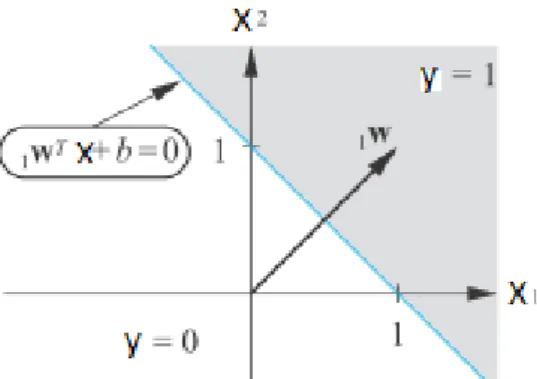
space, which called weight vector, b is a constant value that does not depend on any input value called bias value, and y is output, indicating class label. For a linear classi-fier, the training data is used to learn W and for classifying new data only W is needed. The core idea of the single layer perceptron algorithm is to define the class label of any real-valued numerical input feature Xi, using the sign of the predicted function yi from

the discriminant function yi = W · Xi + b. Let us consider binary classification where

class labels are either y=1 or y=0. Figure 2.1 shows a simple example in a 2-dimensional feature space. It illustrates two different classes and the separating plane corresponding to W·X + b = 0.

(19)

Figure 2. 1. The sign of the projection onto the weight vector W yields the class label

It is clear that the sign of the function W ·X + b determines the class label. Thus, the problem reduces to finding weights W with the use of training examples. The algorithm starts with initializing the weight vector randomly to equal values for all elements, and then updates these initial parameters when applying the current function on the training set makes mistake ‎[68, 59, ‎11,‎ 44, 69]. Learning rate α, where 0 < α ≤ 1 can also be used to adjust the magnitude of the update, for example a too high learning rate makes the perceptron periodically oscillate around the solution.

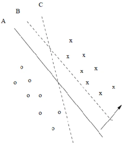
The perceptron approximates a linear function, therefore if the training set is linearly separable; the perceptron is guaranteed to converge. In case the data is not linear sepa-rable then perceptron will not be able to find a good model to separate the data ‎[44]. While the perceptron algorithm finds just any linear separation, Support Vector Ma-chines (SVMs) ‎[10‎, 81] are a kind of classifiers, which search for the best separator to have maximum margin between two groups of data according to some criterion. For example, consider two-class, separated training datasets of ‘x’ and ‘o’ that is illustrated in Figure 2.2 Comparing three different separating hyper-planes denoted by A, B, and C among many others, it is clear that the hyper-plane A provides better separation than the other two which are close to data points of one or both classes, and the normal dis-tance of any of the data points from it, is the largest. Therefore, the hyper-plane A rep-resents the maximum margin to closest points of ‘x’ and ‘o’.

(20)

Figure 2. 2. Finding the best separating hyper-plane

The hyper-plane in SVM is constructed by using a subset of training data that are on the margin. These training data are referred to support vectors ‎[84]. Figure 2.3 shows the margin and support vectors for a sample problem. ‎[28] proposed that ”the ability of SVMs to learn can be independent of the dimensionality of the feature space”. This property causes SVMs to be able to apply for datasets with high dimensionality, if they are separable with a wide margin. In addition, SVMs can also be used for nonlinear classifiers using kernel functions ‎[28].

(21)

For nonlinear separable samples, these techniques have the ability of mapping the orig-inal finite dimensional space into a higher dimensional space using kernels in order to have linearly separable samples. However, ‎[19] mentioned that kernel functions are not so efficient for text classifications since the main assumption for kernels to be effective is that single words are not informative as high order word correlations. But, in some cases linear combination of word occurrences may provide this correlation. Therefore they can be effective for some special problems.

2.3

Literature Review

In general, there are various techniques for detecting network intrusions, signature (or misuse) detection, and anomaly detection [29, 30, 31, 32, ‎35 and‎‎36]. From ‎[36], both signature and anomaly-based detections are similar from conceptual operation point of view yet their main difference is in the nature of attack and anomaly terms. The term of attack refers to “a sequence of operations that puts the security of a system at risk” ‎[36], while an anomaly is defined as “an event that is dubious from security point of view” ‎[36].

In signature detection, the behaviour of a known intrusion or weak spots of a system are modelled to use for detecting known intrusions [29, 30, 31,‎ 32,‎‎33, 34, ‎35 and‎‎36]. High accuracy of detecting known attacks with low false positive rate is the main ad-vantage of this approach. But this approach is not able to detect unknown intrusions. In anomaly detection, normal behaviour of network is modelled and then it compares ac-tivities against the normal behaviour [29, 30, 31,‎ 32, 34, ‎35 and‎‎36]. The advantage of this approach is its ability to detect new intrusions. However, it cannot detect the intru-sions that are not significantly different from normal activities, leading in high false positive rate [29, 30, 31,‎ 32,‎‎33, 34, ‎35, and‎‎36].

Some research groups focused on signature (misuse) detection approaches using differ-ent techniques. For example, ‎[40] introduced a prototype Distributed Intrusion Detec-tion System (DIDS) that worked based on expert systems generating a set of rules that describe known attacks. Then the information from different components is analysed at a central location. ‎[34] represented an example for state transition analysis approach. In this approach the process of intrusions are demonstrated as a series of state changes by using a graphical notation. Researches in ‎[39] focused on developing a domain-specific

(22)

language called behavioural monitoring specification language (BMLS) to determine the relevant properties, from either normal behaviour of systems, or misuse behaviour associated with known attacks. They provide the STAT Tool Suite, which includes a language called STATL to describe the attack scenarios. But the problem of signature (misuse) detection is that it needs frequent rule base updates and signature updates. Nevertheless, this approach is not able to tackle the rapidly increased number of new attacks.

On the other hand, anomaly detection methods that model the normal network behav-iour are relatively easy to perform, and effective in finding both known and unknown attacks. A vast number of researches have been performed on this topic using different methodologies ‎[41, 42, ‎43,‎ 44, 45, ‎46, 50, 51, ‎52, ‎53, ‎54 and‎‎55]. These methods can be categorized into three different groups: statistical-based, specification-based and ma-chine learning-based, which are briefly introduced next.

Statistical-based methods build operational profiles that describe normal behaviour of a system over a period of time. In general, normal profiles include probability distribu-tions of different variables that represent the state of the system. Then a statistical dis-tribution profile of new data is compared to the normal profile to distinguish significant differences and make decision based on this discriminant [‎41, ‎‎42 and ‎43]. The weak-nesses of this method are that it ignores the temporal and multiple-variable correlation [‎67, ‎68].

Specification-based approaches are described in [‎ 44, 45 and ‎46]. In this approach, instead of modelling the normal activity, it builds a model based on specification of a secure operation. Accordingly, if an operation does not resemble this model then it is marked as an intrusion. This approach does not have the drawbacks of statistical-based methods; however it can be infeasible if the size of datasets is too big.

Machine learning can be defined as a programme or system that can learn from data and improve the performance over time. Thus, the strategy of a machine learning based method can change with new data. Necessity for labelled data to train a learning algo-rithm is its unique characteristic. But the ability of this technique to extract information directly from historical data without the need for manual work has attracted a lot of attention concerning intrusion detection. In addition, it can draw patterns over

(23)

incom-plete data and handle a large amount of data. Because of these reasons, variants of ma-chine learning techniques have been applied to intrusion detection systems.

For example Bayesian network is a model that provides capability to capture relation-ships among variables of interest ‎[36]. In general, this technique combined with statis-tical schemes is used for intrusion detections. Researchers in [50, ‎52, ‎53 and ‎54] pro-vide different approaches combining Bayesian network model with variety of statistical values. But from ‎[30], the problem with these methods is it depends on the assumptions about the behavioral model of the system. It means that the detection accuracy depends on the accuracy of chosen model. But finding an accurate model is a challenging task because of the complexity behavioral model within this system.

Clustering is another technique that works by grouping the data based on a given simi-larity or distance measure and characterizes anomalies considering dissimilarities ‎[36]. A similarity measure is a key parameter in clustering to detect anomalies. For example, the k-nearest neighbor approach in ‎[51] uses Euclidean distance to assign data points to a given cluster. Some sophisticated clustering also use fuzzy-k-mean and swarm-k-mean algorithms to improve the local convergence ‎[55]. From ‎[76] the advantage of clustering is its ability to learn from raw data in addition to detect intrusion in raw data without necessity of preprocessing and manual work. But for high dimensional data points it cannot provide the result with high accuracy.

Neural networks are human brain inspired approaches that have been employed for anomaly intrusion detection. Flexibility and adoptability to environmental changes are characteristics of these approaches; however there is not any learnable function ‎[76] for making decision. Various approaches using neural networks for intrusion detection have been introduced by some research groups [59, 60 and 61]. In ‎[62], the Anomalous Network-Traffic Detection with Self Organizing Maps (ANDSOM) was represented, which works based on monitoring a two dimensional Self Organizing Map (SOM) cre-ated for each network service. In training phase neurons are trained using normal net-work traffic. When feeding real time data to trained neurons, an anomaly is detected by comparing the distance of incoming traffic with a present threshold.

Support Vector Machines (SVMs) are another techniques involved in anomaly detec-tions [‎69, 70]. Such techniques use one class learning techniques for SVM and learn a

(24)

region within the feature space with a maximum margin. Many researchers use variants of the basic technique (combined with other methods or different kinds of feature ex-traction methods) for detecting the anomalies in different fields such as computer and telecommunication networks. For example, ‎[63] reports an improvement using SVM to the SOM approach used by ‎[66]. In ‎[65] authors have proposed a new robust approach of SVM for anomaly detection over noisy data. They have shown in their approach that testing time are faster since the number of support vectors is significantly less than compared to standard SVMs.

(25)

3.

METHODOLOGY

The aim of this thesis is to investigate supervised machine learning approaches to de-tect known abnormal log behavior in log files as a fast and efficient approach. As men-tioned in chapter 2, machine learning is the ability of a machine to improve its perfor-mance automatically through learning. A supervised learning technique needs labeled data in order to find a function or model that maps a sample into the class labels. Using labeled data during the training phase enables achieving clear feedbacks that help to learn quickly. Therefore, high efficiency and fast learning are advantages of supervised learning techniques. In addition, it is a powerful approach to detect known failures due to have robust patterns. Therefore, it can be a well suited approach and worth investi-gating for our special case detecting known faults.

In this approach, anomaly detection is considered to be a binary classification since the aim is to identify abnormal cases against normal ones. Thus, labelled data, as either normal or abnormal, is used for the learning phase in order to build detection models (profiles). Such models are employed for identifying the anomaly behaviors. The pri-mary step in learning phase is to collect feature vectors as input data fed to training algorithm. In this approach, we collect feature vectors using sliding window, n-gram (bag-of-words), and word count to learn machine learning classification. From chapter 2, single layer perceptron and SVM are investigated as promising candidate methods of linear classifications for anomaly detection based on the textual characteristics of event logs used in this thesis. The most challenging phase of this investigation was big data including long lasting fault.

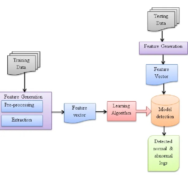
In this chapter, the methodology for generating the detection model is described. As illustrated in Figure 3.1 learning algorithm for building detection model contains fea-ture extraction phase followed by model learning and testing phases to evaluate the accuracy of the detection. In Section 3.1, feature extraction approaches and mining the patterns of logs and prerequisites are defined. In Section 3.2, the approaches for detect-ing short duration faults as well as long lastdetect-ing faults are described.

(26)

Figure 3. 1. Overview of the learning algorithm

3.1

Feature generation

Feature generation is an important part of any classification method. To achieve high quality anomaly detection, it is required to create high quality numerical features, indi-cating the log information which is understandable by machine learning classification. As reviewed in Chapter 2, several approaches for extracting features from log data have been well investigated in the literature. In this project we use windowing along with n-gram (bag-of-words) approach to extract features from event logs considering their textual characteristics. The following sub-sections describe the proposed approach in-vestigated in this thesis.

(27)

3.1.1

Prerequisites

Ground truth: In order to analyse event log data and create labelled training samples, having ground truth is the first requirement. Mainly, ground truth dataset is human-expert knowledge based. It is defined as the labels associated with the data points to indicate if the data represents a problem or a normal case. Furthermore, ground truth can be used to evaluate the method by measuring the degree of match between ground truth labels (desired states) and actual ones obtained from classification methods. Fig-ure 3.2 shows a part of ground truth dataset. Labels 1 indicate the fault logs, while la-bels 0 are associated with normal ones. In the cases that more than one fault is available in the event log data, one ground truth dataset is needed for each fault to allow pro-cessing each fault separately.

Figure 3. 2. A part of ground truth dataset, fault logs labelled as 1 and normal logs labelled as 0

Dictionary: As mentioned before and illustrated in Figure 3.3.a the format of logs (event logs) is not fixed. But there are some similar characteristics between all log mes-sages. A log event typically has a timestamp with a fixed format representing the time at which the software has written the event. A log event also includes at least a text message containing English words, digits, and special characters. In a bag-of-words based feature model creating a dictionary, is a crucial prerequisites. By dictionary we means a collection of terms (i.e., words or phrases), as a reference for collecting numer-ical feature vectors. To do this, first message parts of all logs in a log data are tokenized using for example white-spaces and punctuation as token separators. In order to reduce

(28)

the dimension of dictionary, which relates to reducing the feature vector dimensionali-ty, it is necessary to filter tokens and collect as informative words as possible. Filtering is done by removing digit numbers and special characters. Then by assigning an integer id for each unique English word the desired dictionary is created since English word messages are the most informative parts of logs. Figures 3.3.a and 3.3.b illustrate a log message and its corresponding tokens after filtering which are to create dictionary (col-lection of words)

a. A sequence of log messages

b. Tokens after filtering and a sample of a dictionary as a collection of words

c. Collected strings and a sample of a dictionary as a collection of strings Figure 3. 3. Sequence of logs and their corresponding tokens

However, as the number of logs in a dataset increases, the dimension of dictionary and consequently dimension of feature vectors increases as well. As a result, the processing time significantly increases. To address this problem, using bag-of-strings inspired from n-gram methodology in text processing, instead of bag-of-words is proposed. To do this, each message line is converted to a message with reduced size by concatenating the final desired words (from aforementioned rules) of each line to create a string. As it is illustrated in Figure 3.3.c this approach causes the size of dictionary to reduce from the numbers of unique English words in a log data to the numbers of unique messages in that data, while each term in dictionary refers to a string instead of a word.

(29)

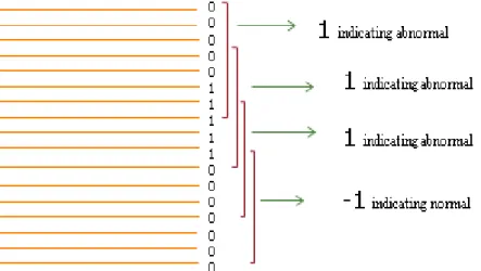
Labelling: As mentioned before, supervised learning needs labelled training data to build a detection model. Therefore it is necessary to assign label to each feature vector collected from raw data. To do this, time series dataset is segmented by windowing while segments are contained a set of labels (from ground truth dataset) associated to sequences of logs in that segment. Each segment is labelled based on the ratio of the numbers of normal logs to abnormal logs while threshold can be changed based on the series experimental results. For example in Figure 3.4 the rule for labelling is consid-ered as one-fifth. It means if one-fifth of logs in each window are faults (labelled as 1) the feature vector corresponding to that window is labelled as fault.

Figure 3. 4.Assign label to each feature vector

3.1.2

Feature Extraction

Our approach for collecting feature vectors is based on combining two strategies of sliding window and bag-of-words. Sliding window as a standard way to deal with streaming data is used to isolate sequential data. In this method, two properties of win-dow size and sliding value need to be specified. The winwin-dow size is used to limit a se-quence of data used for processing to a certain range in time or number of logs. The sliding value is used to specify the execution condition of the processing. Whenever the process of collecting feature from certain window is performed, the sliding window is moved forward by a presumed value to specify next sequence. For instance, consider a

(30)

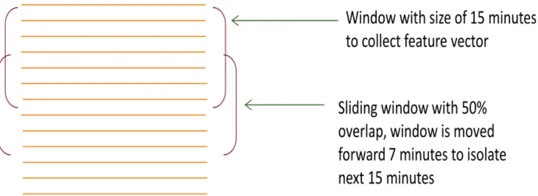
window of fixed size, 15 minutes, (in a time based windowing) and sliding value of 7 minutes (50% overlap) as it is shown in Figure 3.5 This window is placed at the begin-ning of the log file. All logs that fall in that window based on their time stamp are con-sidered to be one sequence and create one feature vector. Then the window is moved forward 7 minutes and the next 15 minutes logs are made into a sequence. In the sce-nario that the duration of the faults is known (to have ground truth) the time based win-dowing is preferred.

Window with size of 15 minutes to collect feature vector

Sliding window with 50% overlap, window is moved forward 7 minutes to isolate next 15 minutes

Figure 3. 5. Sliding window for streaming data

In bag-of-words based feature models, to collect feature vector associated with each segment, certain sequence specified by windowing, we need to tokenize the message parts of all logs in this window applying the same rules (tokenizing, filtering and col-lecting words or strings) used for creating dictionary. Then the number of occurrence of each term from dictionary in each segment is counted and collected as features to create feature vector (feature vectors and dictionary have equal dimension). This notation is called as term frequency in many documents.

For long documents, using raw counts directly particularly for linear classification is not efficient ‎[77], because different numerical features in each feature vector may have different values. As mentioned in Chapter 2, in order to avoid those features with larger values being dominant, normalization is usually required. For normalization we consid-er the occurrence of each tconsid-erm vconsid-ersus the total numbconsid-er of occurrences of all tconsid-erms in a feature vector to scale the term frequencies to values between 0 and 1.

(31)

3.2

Detection phase

Considering the textual characteristics of event logs, linear classification is used, as it is a well-suited method for text processing. Two important factors, the size of datasets and the time duration of faults, are investigated in order to generate an appropriate ap-proach generalizing for detecting known faults. In following sub-sections, first, general approach; learning phase and testing phase used for short fault duration is described. Then in Section 3.2.1, we deal with feature extraction and classification methods for long faults.

3.2.1

General approach – short faults

Fault detection for datasets including short faults like any classification algorithm is implemented in two steps, learning phase and testing phase. The major task of learning phase is to build detection model using training dataset that provides information for detecting anomaly behaviors. In testing phase the performance of learning algorithms and feature extraction methods is evaluated. The testing phase algorithm employs the detection model to classify new dataset that are unknown to the algorithm. Then, de-tected labels are compared to the actual ones to estimate the performance of detection algorithm.

3.2.2

Long fault duration – two-layer classification

Prior to this sub-section, an overall technique for fault detection was described. But for long lasting faults where a large number of logs can be labeled as faults, the mentioned approach is not able to successfully detect such abnormality. In practice, a special case can be when a long fault is repeated several times throughout a dataset while many of them overlap with each other. Such scenario will result in fault reporting for majority of the logs. Two-layer classification with distinct approaches for extracting features in each layer is presented as a solution to address this kind of problem.

Two-layer classification comprises of two layers. The first layer includes two classifi-ers in parallel. For convenient undclassifi-erstanding, we called them based on their character-istics, middle classification and start classification. Middle classification focuses on all abnormal logs while start classification concentrates on starting lines of each fault

(32)

repe-tition. The approach for middle classification is the same as previous ones. Feature vec-tors are collected using the approach mentioned in Section 3.1 while the best detection model from learning phase is required and saved to be used in the second layer.

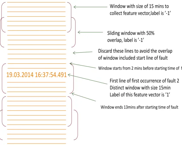
As in start classification the focus is on starting lines of each fault occurrence, a differ-ent approach of extracting features is proposed for this type of classification. As it is shown in Figure 3.6 for extracting features and collecting feature vectors, the window-ing is started from the first line of dataset. The window size and slidwindow-ing value must be the same as what was used for middle classification. However, the windows including first line of each fault must be distinct without any overlap. It is needed to assign a spe-cific window with the same size of others to the range of logs, including starting line of fault, in such a way that the large part of the window includes the logs which come after starting line of fault. For example by considering window size of 15 minutes, we specify the window to start 2 minutes before timestamp of starting line and to terminate 13 minutes after starting line of each repetition of the fault. Then feature vector associ-ated to each window is creassoci-ated using previous method (bag-of-words or bag-of-strings). For labelling, windows containing starting line of each fault are labeled as abnormal and all other windows are labeled as normal. Figure 3.6 shows that discarding some lines is inevitable in this approach in order to avoid an overlap between windows in-cluding start line of each fault and other windows. After collecting feature vectors, detection models is built from learning phase and the best one is saved from testing phase. As an important point, detection model for both middle and start classifications must be created using the same classification method.

(33)

19.03.2014 16:37:54.491

First line of first occurrence of fault 2 Distinct window with size 15min Label of this feature vector is ’1’

Window starts from 2 mins before starting time of fault

Window ends 13mins after starting time of fault Window with size of 15 mins to collect feature vector,label is ’-1’

Sliding window with 50% overlap, label is ’-1’

Discard these lines to avoid the overlap of window included start line of fault

Figure 3. 6. The approach of feature extraction for start classification of first layer

The approach of extracting features for second layer is completely different from what has been used so far. To collect feature vectors of second layer, two detection models produced from first layer are used exploiting the collecting feature vectors approach described in 3.1 Section. In this approach, as faults have overlap to each other the start-ing lines of each fault (which are unique) have critical part/role. Therefore, the last five probability estimation values produced from applying detection model of start-classification provided by first layer are used directly to create each feature vector of second layer.

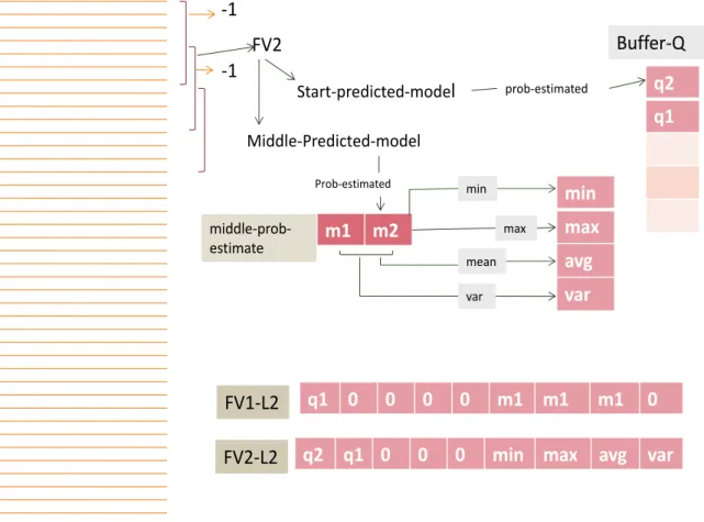
To implement such method, we design a buffer (first input-first output) with size of five in order to save aforementioned values. As illustrated in Figure 3.7, vectors of second layer are considered to have nine dimensions that their first five elements are filled by the values of aforementioned buffer (Buffer-Q). The procedure is started by windowing and creating numerical feature vector for the first window (FV1). Afterwards, two pre-dicted models from first layer are applied on this feature vector.

(34)

FV1 Start-predicted-model Middle-Predicted-model q1 Buffer-Q Buffer-Q prob-estimated m1 middle-prob-estimate m1 m1 m1 0 min max mean var q1 0 0 0 0 m1 m1 m1 0 FV1-L2 Prob-estimated -1 -1

Figure 3. 7. Creating first feature vector of second layer

The probability estimated value obtained by applying Start-classification model (named as Start-predicted-model in Figure 3.7) is saved in the buffer while another vector (middle-prestimate in Figure 3.7) is used to save probability estimated value ob-tained by applying middle-classification model (named as Middle-predicted-model in Figure 3.7) on this feature vector (FV1). This vector is an unlimited vector in order to have the ability of saving probability estimated values of next windows. The statistical values obtained from aforementioned vector such as minimum, maximum, mean, and average value are used to create the feature vector of the second layer. The last step to generate the feature vector is to replace the first five elements of it by buffer (Buffer-Q) values and last four elements of it by statistical values of the second layer. But as it is illustrated in Figure 3.7 for the first feature vector buffer has only one value, and hence, we need to replace the other elements by zeros. Furthermore, there are three equal sta-tistical values for the first feature vector of the second layer (FV1-L2).

For the second feature vector, the aforementioned procedure is performed on the next window. It is depicted in Figure 3.8 that probability estimated value obtained by apply-ing Start-predicted-model on the feature vector of this window is saved in buffer while buffer has also kept the previous value. And statistical values are computed using both

(35)

probability estimated values of applying Middle-predicted-model on feature vector cor-respond to this window and the previous one.

FV2 Start-predicted-model Middle-Predicted-model q2 q1 Buffer-Q Buffer-Q prob-estimated m1 m2 middle-prob-estimate min max avg var min max mean var

q2 q1 0 0 0 min max avg var

FV2-L2 q1 0 0 0 0 m1 m1 m1 0 FV1-L2 Prob-estimated -1 -1

Figure 3. 8. Creating second feature vector of second layer

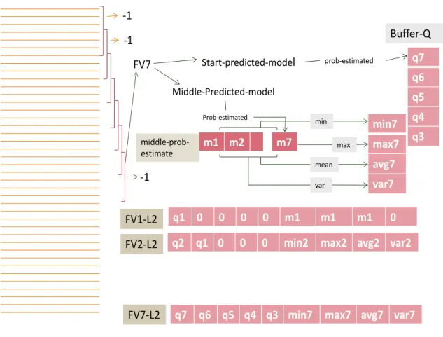
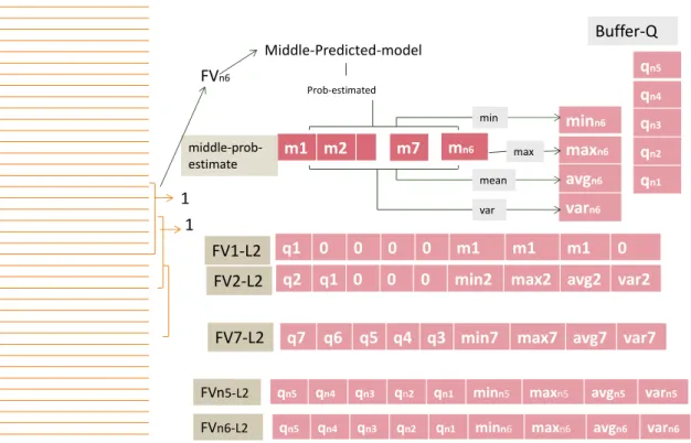
To assign label to each feature vector, we use the approach described in Sub-Section 3.1.1 under the title of labelling. It means both generating feature vector of second layer and labelling them are based on sliding window throughout the main dataset. As it is illustrated in Figure 3.9 the aforementioned procedures continue and next feature vec-tors are built as long as the fault logs have not been detected and all labels indicate the normal cases.

(36)

FV7 Start-predicted-model Middle-Predicted-model q7 q6 q5 q4 q3 Buffer-Q Buffer-Q prob-estimated m1 m2 middle-prob-estimate min7 max7 avg7 var7 min max mean var

q2 q1 0 0 0 min2 max2 avg2 var2

FV2-L2

q1 0 0 0 0 m1 m1 m1 0

FV1-L2

m7

q7 q6 q5 q4 q3 min7 max7 avg7 var7

FV7-L2

Prob-estimated

-1 -1

-1

Figure 3. 9. Feature vectors of second layer consist of last five values from start-predicted-model and statistical values from middle-start-predicted-modelof first layer

When the fault is detected by the label correspond to window, buffer will not update anymore and only the dimension of middle-prob-estimate increases by collecting the probability values of applying middle-Predicted-model to feature vector correspond to each window. Accordingly, as it is seen in Figure 3.10, after indicating fault logs, only the last four elements of feature vectors are updated while the first five elements are fixed. This procedure continues until the end of fault and indicating the normal logs by associated label.

(37)

FVn6 Middle-Predicted-model qn5 qn4 qn3 qn2 qn1 Buffer-Q Buffer-Q m1 m2 middle-prob-estimate minn6 maxn6 avgn6 varn6 min max mean var

q2 q1 0 0 0 min2 max2 avg2 var2

FV2-L2

q1 0 0 0 0 m1 m1 m1 0

FV1-L2

m7

q7 q6 q5 q4 q3 min7 max7 avg7 var7

FV7-L2

Prob-estimated

1 1

mn6

qn5 qn4 qn3 qn2 qn1 minn5 maxn5 avgn5 varn5 FVn5-L2

qn5 qn4 qn3 qn2 qn1 minn6 maxn6 avgn6 varn6 FVn6-L2

Figure 3. 10.After detection of fault logs, only the last four elements of feature vector will be changed

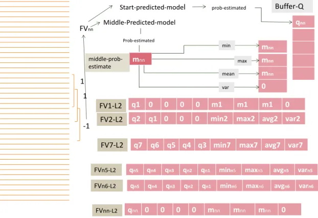
Indicating the normal situation cause both buffer and middle-prob-estimate vector, il-lustrated in Figure 3.11 to reset, and the procedure repeats again from the first step for the rest of data.

After collecting all feature vectors for second layer the detection model is created by applying the same learning algorithm with the exact parameters used for first layer on the training data obtained from second layer. And then this approach is evaluated by applying aforementioned model on the testing samples.

(38)

FVnn Middle-Predicted-model qnn Buffer-Q Buffer-Q mnn middle-prob-estimate mnn mnn mnn 0 min max mean var

q2 q1 0 0 0 min2 max2 avg2 var2

FV2-L2

q1 0 0 0 0 m1 m1 m1 0

FV1-L2

q7 q6 q5 q4 q3 min7 max7 avg7 var7 FV7-L2

Prob-estimated

1

qn5 qn4 qn3 qn2 qn1 minn5 maxn5 avgn5 varn5 FVn5-L2

qn5 qn4 qn3 qn2 qn1 minn6 maxn6 avgn6 varn6 FVn6-L2 -1 1 Start-predicted-model prob-estimated qnn 0 0 0 0 mnn mnn mnn 0 FVnn-L2

Figure 3. 11. By ending the fault logs and indicating normal logs both buffer and mid-dle-prob-estimate reset and procedure starts from first step

(39)

4.

RESULTS

In this chapter, we present the experimental results for our proposed fault detection technique over two dataset. We first describe the dataset characteristics and evaluation measures used for our experiments, and then present the results and discuss the perfor-mance of the detection method considering different factors.

4.1

Data

We did experiments using two different datasets, TTY and TTY-2, and compare two classifier methods considering the effects of different factors. The datasets used in this thesis are generated by TIETO using a simulator with a real cellular (3G/4G) network structure from Poland1. The log data contains more than traffic data. It may also include diagnosis data, system status report, error report, system performance report, and so one. The data is collected from both mobile core network and other peripheral parts, such as base stations. The faults simulated in the data are related to software, hardware, and network connection faults as well as configuration problems in the 4G network base stations. Software faults might relate to license expiring whereas hardware related issues might be network connections lost, HDD failures or access/write problems. TTY dataset with 500330 logs is chosen to evaluate two classifier methods, single layer Perceptron and SVMs. It contains two days of network traffic data, which includes a fault with a duration time of around 16 minutes that repeats 20 times throughout the dataset. This fault is related to the base station base bandwidth failure.

TTY-2 dataset with 516691 logs contains five days of network traffic data including five different faults each one repeats 20 times throughout the dataset. These faults have different duration time around 8 milliseconds, 2 minutes, 5 minutes, 16 minutes and the most challenging fault has 36 hours duration. Thus, its 20 time repetitions cause to have a dominant fault with near 5 days duration. The faults included station base bandwidth

(40)

failure, software licensing alarm issue, a faulty configuration file, a broken cable con-nection, and BCCH missing alarm. TTY-2 is chosen to investigate the effect of fault duration factor on classifier method and generate a proper approach for long lasting faults.

For each experiment a time series data together with a configuration file that defines the duration time of each fault and its repetition times are available. For example, from Figure 4.1, time distance between first pair of lines (difference between two timestamps) shows the fault duration for the nineteenth repetition of the fault with id equal to 1. Second pair of lines indicates that fault with id 1 has been repeated twenty times in total. Hence, the next pair of lines represents the timestamps of the fault with id 2. This file is used to provide ground truth dataset required for supervised learning methods.

Figure 4. 1. A part of Fault List Log illustrating two different faults, and time duration of each repetition

4.2

Evaluation measures

As mentioned in chapter 3, in order to evaluate detection models, we need to reserve a portion of data for the test set. In our early experiments we manually split the dataset into two parts as training dataset and testing dataset. But for cases that fault logs are not equally distributed throughout the dataset or the number of one class is very small in compare to other class it is probable that one of the sets for training or testing might miss a certain class. Therefore, this method for collecting training and testing samples

(41)

cannot provide a proper approach to assess the detection model. Instead Cross valida-tion‎[47] is a technique used to overcome this shortage and to select the optimal detec-tion model ‎[2] and estimate the accuracy performance of classifiers. By using this tech-nique, feature vectors collected from entire dataset are partitioned into complementary subsets (or folds). One set is considered as testing set or validation set and used to eval-uate the created model. While the other subsets called training set, are used to create the detection model. In addition, to evaluate the performance of learning algorithms we need to choose metric measures that are able to measure the best performance of learn-ing algorithms. In literature, accuracy and error rate are two common criterion func-tions to assess classifier performance in order to find the best detection model. Accura-cy defines the percentage of correct classifications, while error rate is the percentage of incorrect classifications. But they may not well suited for evaluating models created from imbalanced datasets when the number of abnormal logs is much less than the number of normal logs. For example in a dataset that consists of 100 logs in total and only one abnormal log, for detection results indicating all logs as normal the accuracy will be 99%. While this result represents low quality of model as it cannot detect any faults in dataset. Instead, precision and recall are two evaluation functions that focused on the number of detected faults ‎[28]. To define these two evaluation metrics first we need to introduce the confusion matrix that represents the prediction results. Confusion matrix is a table where each cell [i,j] indicates the number of times that j was predicted when the correct label was i. Figure 4.2 shows a confusion matrix where:

 True negative (TN) corresponds to the number of normal logs correctly predict-ed by the learning method.

 True Positive (TP) corresponds to the number of abnormal logs correctly pre-dicted by the learning method.

 False Negative (FN) corresponds to the number of abnormal logs wrongly pre-dicted as normal logs by the learning method.

 False positive (FP) corresponds to the number of normal logs wrongly predicted as abnormal logs by the learning method.

(42)

Figure 4. 2. Confusion Matrix

Thus, the diagonal elements indicate labels that were correctly predicted and the off-diagonal elements indicate errors. Precision represents the fraction of real abnormal logs from all predicted abnormal logs by a classifier method. High precision means that learning method rarely predicts normal logs as abnormal logs. Recall measures the frac-tion of abnormal logs that are correctly predicted by classifier method. High recall means that learning method rarely predicts abnormal logs as normal logs.