Using a Unified Measure Function for Heuristics,
Discretization, and Rule Quality Evaluation in
Ant-Miner
Khalid M. Salama
School of Computing University of Kent Canterbury, CT2 7NF, UK Email: [email protected]Fernando E. B. Otero
School of Computing University of KentChatham Maritime, ME4 4AG, UK Email: [email protected]
Abstract—Ant-Miner is a classification rule discovery algo-rithm that is based on Ant Colony Optimization (ACO) meta-heuristic. cAnt-Miner is the extended version of the algorithm that handles continuous attributes on-the-fly during the rule construction process, while µAnt-Miner is an extension of the algorithm that selects the rule class prior to its construction, and utilizes multiple pheromone types, one for each permitted rule class. In this paper, we combine these two algorithms to derive a new approach for learning classification rules using ACO. The proposed approach is based on using the measure function for 1) computing the heuristics for rule term selection, 2) a criteria for discretizing continuous attributes, and 3) evaluating the quality of the constructed rule for pheromone update as well. We explore the effect of using different measure functions for on the output model in terms of predictive accuracy and model size. Empirical evaluations found that hypothesis of different functions produce different results are acceptable according to Friedman’s statistical test.
I. INTRODUCTION
Data mining is a process that supports knowledge discov-ery by finding hidden patterns, associations and constructing analytical models from databases [1]. Classification is one of the widely studied data mining tasks in which the aim is to discover, from labeled cases, a model that can be used to predict the class of unlabeled cases. Ant-Miner, proposed by Parpinelli et al. [2], is the first ACO algorithm for discovering classification rules of the form:
IF<Term-1> AND<Term-2> AND. . . THEN<Class>, where each term is represented as an(attribute=value)pair, and the consequent of a rule corresponds to the class value to be predicted. Ant-Miner has been shown to be competitive with well-known classification algorithms, in terms of pro-ducing comprehensible model with high predictive accuracy. Therefore, there has been an increasing interest in improving the Ant-Miner algorithm. Nonetheless, the majority extended versions of the algorithm introduced in the literature have an important limitation of only being able to process nominal attributes, whilst in practice most real-world classification problems involve both nominal and continuous attributes.
Thus,cAnt-Miner was presented by Otero et al. [3], [4] as a variation of the original algorithm, which is able to cope
with continuous-valued attributes during the rule construction process through the creation of discrete intervals on-the-fly. The discretization was performed based on entropy and Minimum Description Length (MDL) to create two intervals [3], or several intervals from the continuous attribute and selecting the best interval [4].
On the other hand, Salama et al. recently introduced an ef-ficient version of the algorithm,µAnt-Miner [5], [6], based on selecting the consequent class of the rule before constructing its antecedent and utilizing multiple pheromone types, one for each permitted rule class. This motivated the idea of utilizing the pre-selected class in heuristic information calculation, and continuous attribute discretization.
From this ground, in this paper we combine cAnt-Miner with µAnt-Miner to fabricate a novel approach for learning classification rules via ant-based optimization. The proposed approach is built upon the notion of using a unified classifi-cation measure function in three essential aspects of the algo-rithm. First, the heuristic information of a term is computed by this measure function. Second, we use the same measure function as criteria for discretizing continuous attributes and dynamically creating intervals during rule construction. Third, the quality of the constructed rule is evaluated for pheromone update also using this unified measure function.
In addition, we explore how the use of different measure functions affects the quality of the produced classification model in terms of predictive accuracy and model size. We examined eight different measure functions, where each played the rule of the unified measure function in the three aforemen-tioned aspects of the algorithm, on 22 UCI datasets.
The rest of the paper is organized as follows. In Section II, we briefly discuss both cAnt-Miner and µAnt-Miner as a foundation of our research. Section III describes in detail our proposed learning approach. Section IV discusses our experimental methodology, where the results are shown in Section V. Finally, conclusions and future work suggestions are presented in Section VI.
II. BACKGROUND
Although Ant-Miner has several extensions, presented and discussed in recent surveys [7], [8], we build our approach upon two recently introduced extended versions of the algo-rithm, namelycAnt-Miner andµAnt-Miner. It is recommended for the reader to have a background on these two algorithm in order to understand the foundation of the extensions proposed in the current work [3], [4], [5], [6].
Otero et al. have introduced two versions of thecAnt-Miner algorithm to dynamically discretize the continuous attributes during the rule construction process. The first version ofc Ant-Miner [3] produces two intervals from a continuous attribute, while the second version [4] produces several intervals to select the best to create a real-valued term to be added to the constructed rule.cAnt-Miner creates thresholds on continuous attributes’ domain values during the rule construction process, producing terms of the form(ai< v)or(ai≥v), whereaiis a continuous attribute andvis a threshold value. The threshold value is dynamically generated using binary discretization (in the first version) or MDL-based discretization (in the second version). These discretization techniques are based on information theory, discussed in [9].
The use of multiple pheromones was introduced in µ Ant-Miner [5], [6] as an extension to the original algorithm. The motivation behind the multi-pheromone system is based on the following hypothesis: the selection of the terms (in the rule antecedent) that are relevant to the prediction of a specific class (rule consequent) constructs better rules than selecting terms simply to reduce the entropy among the class distribution on the dataset, as in the original Ant-Miner. Therefore, it was proposed to select the class of the rule first, and then select the rule’s antecedent terms based on this selected class. On the other hand, sharing pheromone information among ants constructing rules with different classes can negatively affect the quality of the constructed rules, as the terms that lead to construct a good rule for class Cx as a consequent do not necessarily lead to construct a good rule for Cy as a consequent. Hence, using multiple pheromone types is related to the selection of the rule’s consequent class prior to the rule’s antecedent construction.
III. PROPOSEDLEARNINGAPPROACH
In this approach, we employ the µAnt-Miner’s idea of selecting the class before the rule’s antecedent construction, to extendcAnt-Miner in three essential aspects of the algorithms, using a unified class-based measure function. First, we use this unified measure function to compute the heuristic information of the terms to be selected to construct the rule’s antecedent. Second, we use the same function as criteria to carry out the dynamic discretization of the continuous attributes and select the best created interval with respect to the pre-selected class. Third, we use this unified measure function, used for both pervious operations, to evaluate the quality of the constructed rule for the sake of pheromone update. What we mean by class-based measure function is a function that calculates the
quality of a rule (or a term) with respect to a class value— rather than entropy, MDL or information gain.
The rationale behind using a unified measure function (i.e. using the same function used in rule quality evaluation to compute the term’s heuristic information, and as a criterion to discretize and construct intervals for continuous) is the following. Since we evaluate the quality of a constructed rule with a given function fx, there is no need to select terms that maximize another functionfy. Intuitively, the selection of terms that maximizefxshould lead to construct a high quality rule with respect tofx. Moreover, using class-based evaluation function for heuristic information calculation and continuous attributes discretization should lead to the selection of terms that are relevant to the prediction of a specific class, rather than selecting terms simply to reduce the entropy among the class distribution on the dataset as in cAnt-Miner. Therefore, we use a unified quality evaluation functionQEF to compute the heuristic information of a term, to create intervals from continuous attributes in the discretization, with respect to the pre-selected class value, and to evaluate the quality of the constructed rule as well.
Note that, it is possible in our approach to use class-based functions for heuristic information calculation and as a criterion for discretizing continuous attributes only as we take advantage of theµAnt-Miner’s idea of class pre-selection. Thus, we explore how the use of different measure functions in all these aforementioned aspects of the algorithm affects the quality of the produced classification model in terms of its predictive accuracy.
A. Extended Algorithm Overview
Algorithm 1 draws the outline of our extended approach. As shown, the selection of the class to be predicted by a rule takes place before its antecedent construction. At the beginning of the execution of the algorithm, pheromone levels for every class value are initialized. Then, the algorithm enters an iterative(while)loop, where heuristic information is computed for each term with respect to each value of the class attribute using the unified quality evaluation function (QEF). Each anti constructs a rule as follows. First, the class value to be predicted by the rule is selected probabilistically according to pheromone and heuristic information associated with the different class values. Then, the antecedent of the rule is constructed by selecting terms based on pheromone and heuristic information associated with the previously selected class value, using the following state transition formula:
P robability(termij,k) = τij,k·ηij,k Pa r=1 Pbr s=1(τrs,k·ηrs,k) , (1) whereηij,k is the heuristic information fortermij given that class k has been selected. τij,k is the pheromone amount of type classk associated withtermij.
We can claim that the amount of pheromoneτij,k is a direct representation of the quality of termij in the prediction of classkwith respect toQEF function. This is induced by the
Algorithm 1 The Extended Multi-pheromonecAnt-Miner Begin
QEF ←quality evlaution f unction; training set←all training examples; rule list←φ;
InitializeP heromoneAmounts();
while |training set|> max uncovered examplesdo
CalculateHeuristicInf ormation(QEF); Rbest←φ;
Qbest←φ; repeat
Rlbest←φ; Qlbest←φ; fori←1to colony sizedo
SelectRuleClass(anti); Ri ←anti.ConstructAntecedent(QEF); Ri ←P runeRule(Ri, QEF); Qi←QEF.CalculateRuleQuality(Ri); ifQi> Qlbest then Rlbest←Ri; Qlbest←Qi; end if i←i+ 1; end for
anti.U pdateP heromone(Qlbes); if Qlbest> Qbest then
Rbest←Rlbest; Qbest←Qlbest; end if
untilmax iterations orConvergence()
append Rbest torule list;
training set←training set−Examples(Rbest);
ReinitializeP heromoneAmounts(Class(Rbest)); end while
End
fact thatτij,kis the amount of the pheromone dropped – so for – by the ants that selectedtermij to construct rules with class
kas a consequent, and evaluated the quality of these rules with the QEF measure function, to increase the pheromone level on trermij,k according to the rules’ quality.
When a continuous attributes is selected, a term should be constructed in the form of (ai < vupper), (ai ≥ vlower) or (vlower ≤ ai < vupper) by dynamically generating the thresholds vlower and vlower. After each anti constructs a rule, it undergoes a pruning process, same used incAnt-Miner [4], and the quality of the rule is evaluated using the unified measure function,QEF. Only the ant that constructed the best rule in the colony (Rlbest) updates the pheromone level on the construction graph, using the pheromone type corresponding to the class value of the rule. This concludes a single iteration of the (repeat−until)loop.
At the completion of the loop, the best rule (Rbest) con-structed in the colony is added to the list of discovered rules and the examples covered by that rule are removed from the training set. This iterative process is performed until the remaining examples in the training set are less than a user-defined maximum number of uncovered examples, or until a
maximum number of iterations is reached.
B. Computing Heuristic Information
The heuristic information is a value associated with each term, which influences its selection during the rule’s an-tecedent construction according to Equation 1. In our proposed approach, as we take advantage of selecting the class value before selecting the terms for the rule antecedent, we use a three dimensional structure (attribute i, value j, class k) to store the heuristic information for each termij with respect to class k, annotated by ηij,k. By this way, the heuristic information gives a direct clue of thequalityoftermij with respect to class k.
In order to compute ηij,k, we construct a temporary rule with only termij in its antecedent and with class k as a consequent. Then we evaluate the quality of this rule using the unifiedQEF measure function, which gives us the heuristic information value fortermij with respect to classk.
C. How the New Discretization Works
In our extended algorithm, we propose a new method for locating a threshold value in the continuous attribute domain. Taking advantage of the pre-selected class value, we aim to select a threshold value that generates the partitions with high relevance for predicting this specific pre-selected class. This is unlike the original version ofcAnt-Miner, where the threshold value is selected only to minimize the entropy among all the class values. In essence, we calculate a “discrimination” value for each value v in the boundary points of the continuous attributeai given classk, as follows:
disc(ai, v, k) =|Q(Sai<v, k)−Q(Sai≥v, k)|, (2) whereQ(Sai<v, k)and Q(Sai≥v, k) represent the quality of intervalsSai<v andSai≥vrespectively with respect to the pre-selected classk, and are calculated using the unified measure function QEF. As shown in Equation 3, we calculate the absolute difference in quality (measured in terms of QEF) between the upper and the lower intervals of the candidate value vi. The idea is to select the threshold value vbest that maximizes the quality discrimination – with respect to the current selected class value – between the two intervals.
In order to discretize the values in the continuous attribute domain we have two options: 1) generating two intervals, 2) generating multiple intervals from its domain of values. The former we call Binary Interval Discretization (BID) and the latter we call Multi-Interval Discretization (MID).
As for the BID, after locating the threshold that produces the highest quality discrimination value, we select the relational operator that produces the interval with the higher value in terms ofQEF. i.e. ifQ(Sai<vbest, k)> Q(Sai≥vbest, k), then the generated term would be (ai < vbest), else it would be (ai ≥ vbest). Finally, the interval that has the highest value of QEF is selected, this value is also considered as a heuristic information for the continuous attribute nodeai in the construction graph.
TABLE I
DESCRIPTION OF THEQUALITYEVALUATIONFUNCTIONSUSED INEXPERIMENTS. Quality Evaluation Function Symbol Formula
Certainty Factor t (A,B) (A) −(B) 1−(B) Collective Strength c (AB)+(AB) (A)·(B)+(A)·(B) × 1−(A)·(B)+(A)∗(B) 1−(AB)+(AB) f-Measure f 1.5× (AB) (A) · (AB) (B) (AB) (A) 0.5 +(AB(B)) Jaccard δ (A)+((BA,B) ) −(A,B)
Kappa κ (A,B)+(A,B)−
(A)·(B)+(A)·(B) 1−(A)·(B)+(A)·(B) klosgen ω (AB)0.5×(AB) (A) −(B) m-Estimate m (AB)+0.5·(B) (A)+0.5 R-Cost r 2·(A, B)−(A)
Sensitivity × Specificity o (A,B)
(B) × (A,B)
(B)
Support + Confidence s (A, B) +(A,B(A))
On the other hand, when using MID, we repeat the BID procedure recursively on both of the generated intervals, until we there is no increase in the quality of the generated intervals in terms ofQEF or the generated intervals contains example less than min_examaples_per_rule parameter. After-wards, we can have potentially multiple threshold values. In order to select the best threshold value(s), the list of threshold values is sorted and the quality – according to QEF – for each discrete interval is calculated. Then, the interval with the highest value is selected. If an internal interval is selected (an interval between two threshold values), a term in the form
(vj ≤ai< vj+1)is generated; otherwise, a term in the form
(ai < vj) or (yi ≥ vj) is generated (where j is thej−th threshold value selected).
We note that the number of boundary points for selecting the threshold in our approach is generally less than or equal to the number of boundary points in cAnt-Miner. In our approach, we are only interested in a boundary pointTin the range ofai, given that class k is selected, if in the sequence of examples sorted by the value ofai, there are two examplese1, e2∈S
having different classes, such that ai(e1) < T < ai(e2)and one of these two classes is k. Therefore, the time needed for locating the thresholdvbest is reduced, since fewer candidate boundary points need to be evaluated.
D. Exploring Different Measure Functions
We aim to explore how the use of different measure func-tions (QEF) affects the quality of the produced classification model in terms of its predictive accuracy.
The use of different functions only for rule quality evalua-tion has been studied in [10], where the heuristic informaevalua-tion was discarded and continuous attributes were not used. How-ever, in this paper we explore the use of different functions in
our new unified approach, i.e., for heuristics information cal-culation, continuous attributes discretization and rule quality evaluation. Besides, we extend the number of datasets used in our experiments from 13 to 22 (compared to [10]), to include datasets with continuous attributes without prior discretization step.
Table I describes the measure functions used in our exper-iments. The formulas shown use the following terms:
• (A) is the ratio of the number of cases that match the
rule antecedent to the size of the training set.
• (B) is the ratio of the number of cases that match the
rule consequent to the size of the training set.
• (A)is the ratio of the number of cases that do not match
the rule antecedent to the size of the training set.
• (B)is the ratio of the number of cases that do not match
the rule consequent to the size of the training set.
• (A, B) is the ratio of the number of cases that match
both the rule antecedent and consequent to the size of the training set.
• (A, B) is the ratio of the number of cases that neither
match the rule antecedent nor the consequent to the size of the training set.
• (A, B)is the ratio of the number of cases that match the
rule antecedent but do not match the rule consequent to the size of the training set.
• (A, B) is the ratio of the number of cases that do not
match the rule antecedent but match the rule consequent to the size of the training set.
IV. EXPERIMENTALMETHODOLOGY
In order to evaluate the effect of different quality evaluation functions, we have selected 22 datasets from the UCI Irvine machine learning repository [11]. Table II shows a summary
of the selected datasets. All experiments were conducted running a well-known 10-fold cross-validation procedure. For the experiments concerning the binary interval discretization procedure, we have selected thecAnt-Miner2 algorithm as our baseline (denoted ascAM2); for the ones concerning the multi-interval discretization procedure, we have selected the c Ant-Miner2MDLalgorithm as our baseline (denoted ascAM2MDL).
The details of these algorithms can be found in [3], [4]. The proposed extensions of cAnt-Miner using the quality functions presented in Table I are denoted by the correspon-dent quality evaluation function symbol. Since all algorithms used in our experiments are stochastic algorithms, they are run 10 times for each partition of the cross-validation.
We have compared the performance of the algorithms with respect to predictive accuracy and simplicity of the discovered rule lists (measured as the total number of terms in the dis-covered list). In all experiments, the user-defined parameters were set to: colony size = 10, maximum iterations = 1500,
minimum covered cases= 10andmaximum uncovered
exam-ples= 10; no attempt was made to optimize these parameters for each individual dataset.
V. RESULTS ANDANALYSIS
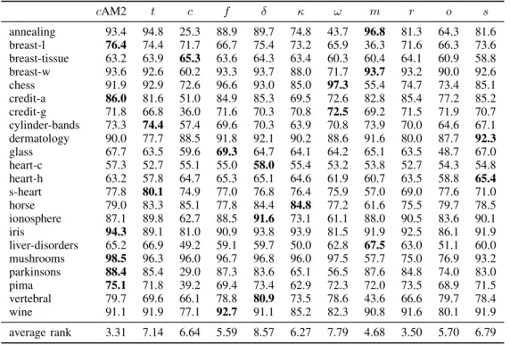
Tables III and IV summarizes the results comparing the predictive accuracy of the algorithms using a binary-interval discretization strategy and multi-interval discretization strat-egy, respectively. Tables V and VI summarizes the results comparing the simplicity of the discovered lists of the algo-rithms using a binary-interval discretization strategy and multi-interval discretization strategy, respectively. The entry shown in bold-face represents the best value obtained for a given dataset.
The last row in each table shows the average rank for each measure function. The average rank for a given algorithm g
is obtained by first computing the rank of g on each dataset individually. The individual ranks are then averaged across all datasets to obtain the overall average rank. Note that, in case of predictive accuracy, the lower the value of the rank, the better the algorithm. The nonparametric Friedman test [12], [13] was applied on the performance average rankings the measure functions used in our experiments.
Concerning the predictive accuracy, there is no algorithm that performs absolutely best, although we have found that some extensions of µAnt-Miner perform statistically signifi-cantly worse according to the Friedman test with the Holm’s post hoc test. The use of Kappa, Collective Strength, Confi-dence, Certainty Factor, Klosgen, and Jaccard in µAnt-Miner resulted in a decrease in performance that is statistically significantly worse (at the α= 0.05level) thancAnt-Miner2, in the case of binary-interval discretization, and statistically significantly worse (at the α = 0.05 level) than c Ant-Miner2MDL, in the case of multi-interval discretization; the
use of F-Measure resulted in a decrease in performance that is statistically significantly worse (at the α= 0.05level) than
cAnt-Miner2, in the case of multi-interval discretization.
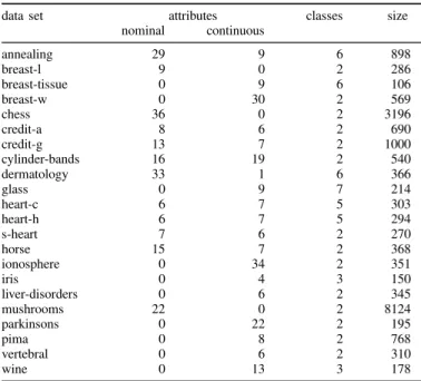
TABLE II
SUMMARY OF THE DATA SETS USED IN OUR EXPERIMENTS.
data set attributes classes size
nominal continuous annealing 29 9 6 898 breast-l 9 0 2 286 breast-tissue 0 9 6 106 breast-w 0 30 2 569 chess 36 0 2 3196 credit-a 8 6 2 690 credit-g 13 7 2 1000 cylinder-bands 16 19 2 540 dermatology 33 1 6 366 glass 0 9 7 214 heart-c 6 7 5 303 heart-h 6 7 5 294 s-heart 7 6 2 270 horse 15 7 2 368 ionosphere 0 34 2 351 iris 0 4 3 150 liver-disorders 0 6 2 345 mushrooms 22 0 2 8124 parkinsons 0 22 2 195 pima 0 8 2 768 vertebral 0 6 2 310 wine 0 13 3 178
Concerning the simplicity, there are four variations ofµ Ant-Miner that have consistently discovered simpler rule lists, namely R-Cost, Kappa, Sensitivity × Specificity, Jaccard and support + confidence. All the remaining, including the baselinescAnt-Miner2 andcAnt-Miner2MDL, have discovered
statistically significantly larger (at the α = 0.05 level) rule lists thancAnt-Miner’s extension using the Collective Strength function.
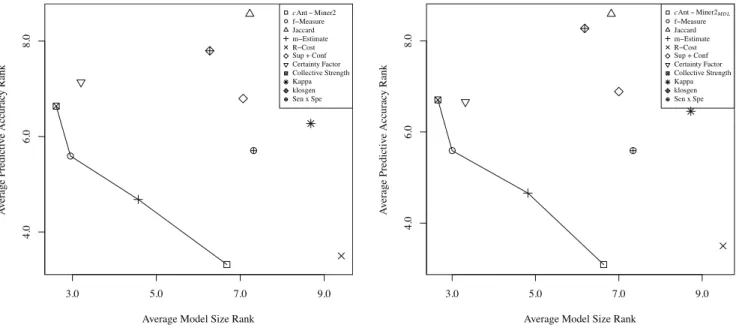
We say a measure function h is dominated by another measure function g if g is better than h in both predictive accuracy and model size. A measure functiong is said to be Pareto-optimal if it is not dominated by any other competing evaluation function-this meansg cannot be improved upon in any one performance measure without sacrificing in another performance measure. The set of Pareto-optimal functions are said to form a Pareto-frontier.
Fig. 1 shows an illustrative plot based on the average accuracy and size rankings. In this figure, the y-axis represents the average accuracy ranking, the x-axis represents the average size ranking, and each measure function is represented as a data-point. The graph on the left represents the binary-interval discretization strategy (BID), while the graph on the right represents the multi-interval discretization strategy (MID). The connected line shows a Pareto-frontier in each of the two strategies with respect to predictive accuracy and model size. Collective Strength, f-measure, m-Estimate andcAnt-Miner2 represent the Pareto-frontier in both BID and MID.
VI. CONCLUSION
In this paper we presented a study of the effect, with respect to predictive accuracy and simplicity of the discovered rule list, of different quality evaluation functions in an ACO
clas-TABLE III
AVERAGE PREDICTIVE ACCURACY(%)USING THE BINARY-INTERVAL DISCRETIZATION PROCEDURE(BID).
cAM2 t c f δ κ ω m r o s annealing 93.4 94.8 25.3 88.9 89.7 74.8 43.7 96.8 81.3 64.3 81.6 breast-l 76.4 74.4 71.7 66.7 75.4 73.2 65.9 36.3 71.6 66.3 73.6 breast-tissue 63.2 63.9 65.3 63.6 64.3 63.4 60.3 60.4 64.1 60.9 58.8 breast-w 93.6 92.6 60.2 93.3 93.7 88.0 71.7 93.7 93.2 90.0 92.6 chess 91.9 92.9 72.6 96.6 93.0 85.0 97.3 55.4 74.7 73.4 85.1 credit-a 86.0 81.6 51.0 84.9 85.3 69.5 72.6 82.8 85.4 77.2 85.2 credit-g 71.8 66.8 36.0 71.6 70.3 70.8 72.5 69.2 71.5 71.9 70.7 cylinder-bands 73.3 74.4 57.4 69.6 70.3 63.9 70.8 73.9 70.0 64.6 67.1 dermatology 90.0 77.7 88.5 91.8 92.1 90.2 88.6 91.6 80.0 87.7 92.3 glass 67.7 63.5 59.6 69.3 64.7 64.1 64.2 65.1 63.5 48.7 67.0 heart-c 57.3 52.7 55.1 55.0 58.0 55.4 53.2 53.8 52.7 54.3 54.8 heart-h 63.2 57.8 64.7 65.3 65.1 64.6 61.9 60.7 63.5 58.8 65.4 s-heart 77.8 80.1 74.9 77.0 76.8 76.4 75.9 57.0 69.0 77.6 71.0 horse 79.0 83.3 85.1 77.8 84.4 84.8 77.2 61.6 75.5 79.7 78.5 ionosphere 87.1 89.8 62.7 88.5 91.6 73.1 61.1 88.0 90.5 83.6 90.1 iris 94.3 89.1 81.0 90.9 93.8 93.9 81.5 91.9 92.5 86.1 91.9 liver-disorders 65.2 66.9 49.2 59.1 59.7 50.0 62.8 67.5 63.0 51.1 60.0 mushrooms 98.5 96.3 96.0 96.7 96.8 96.0 97.5 57.7 75.0 76.9 93.2 parkinsons 88.4 85.4 29.0 87.3 83.6 65.1 56.5 87.6 84.8 74.0 83.0 pima 75.1 71.8 39.2 69.4 73.4 62.9 72.3 72.0 73.5 68.9 71.5 vertebral 79.7 69.6 66.1 78.8 80.9 73.5 78.6 43.6 66.6 79.7 78.4 wine 91.1 91.9 77.1 92.7 91.1 85.2 82.3 90.8 91.6 80.1 91.9 average rank 3.31 7.14 6.64 5.59 8.57 6.27 7.79 4.68 3.50 5.70 6.79 TABLE IV
AVERAGE PREDICTIVE ACCURACY(%)USING THE MULTI-INTERVAL DISCRETIZATION PROCEDURE(MID).
cAM2MDL t c f δ κ ω m r o s annealing 94.3 94.9 25.3 89.0 89.7 78.0 49.2 96.6 81.4 65.0 81.6 breast-l 76.4 74.8 71.8 66.2 74.9 73.3 66.2 36.6 71.2 65.1 73.9 breast-tissue 66.4 61.5 65.3 64.0 63.9 62.9 59.2 60.4 62.8 60.3 59.4 breast-w 93.6 92.6 61.1 93.4 93.9 86.4 74.3 94.1 93.3 90.2 92.8 chess 91.9 92.4 74.2 96.7 93.1 86.9 97.4 59.6 78.6 71.8 84.5 credit-a 86.2 81.9 50.4 85.3 85.3 68.2 70.7 81.7 85.4 76.4 85.2 credit-g 71.7 66.8 35.7 71.3 70.3 70.6 72.3 69.6 71.3 71.3 70.6 cylinder-bands 72.1 73.9 53.1 69.8 70.1 63.7 70.7 72.8 70.1 65.2 66.7 dermatology 89.3 77.9 89.0 91.4 92.2 89.6 89.7 91.1 79.6 88.3 91.6 glass 69.5 64.7 57.5 70.2 65.0 63.8 64.3 65.0 62.4 48.7 66.0 heart-c 57.1 53.3 54.9 55.8 58.3 55.3 54.7 52.7 51.9 53.6 54.3 heart-h 63.9 56.7 64.5 64.6 64.8 65.2 61.3 60.6 63.8 55.8 65.5 s-heart 78.5 79.7 74.4 76.2 76.7 75.3 75.8 58.4 69.7 77.1 71.1 horse 79.2 82.4 85.0 77.5 84.4 84.7 77.7 59.7 75.3 79.1 79.4 ionosphere 87.0 88.2 62.5 88.5 91.9 70.4 62.8 88.7 90.9 83.1 90.1 iris 94.4 89.5 80.9 91.3 94.0 93.9 79.9 91.8 92.6 85.3 91.9 liver-disorders 65.4 68.1 48.5 59.3 59.7 50.6 64.4 68.9 63.1 51.3 60.0 mushrooms 98.4 96.5 96.3 96.8 96.8 96.2 97.6 57.3 74.9 75.6 93.5 parkinsons 88.2 85.5 28.3 86.5 83.3 64.0 55.9 87.5 84.2 74.3 82.9 pima 74.2 71.8 36.7 69.3 73.4 61.7 72.2 70.6 73.9 69.9 71.7 vertebral 79.7 69.8 66.2 79.4 80.8 73.5 80.0 45.4 63.6 78.9 78.8 wine 89.8 91.6 75.1 93.0 91.3 85.9 83.0 91.2 92.2 81.8 92.2 average rank 3.10 6.66 6.70 5.59 8.59 6.45 8.27 4.66 3.50 5.60 6.89
TABLE V
AVERAGE NUMBER OF TERMS IN THE DISCOVERED LIST USING USING BINARY-INTERVAL DISCRETIZATION PROCEDURE(BID).
cAM2 t c f δ κ ω m r o s annealing 13.6 54.8 31.5 8.1 7.0 28.2 28.4 33.6 9.0 17.1 6.3 breast-l 7.5 5.6 2.9 55.1 3.1 5.1 57.2 25.4 6.2 35.9 7.3 breast-tissue 7.9 14.0 6.3 9.9 8.0 8.8 7.9 13.5 6.0 7.3 12.1 breast-w 9.9 46.7 8.4 14.8 3.3 8.1 13.4 29.0 3.2 8.0 4.9 chess 11.6 7.5 2.6 88.5 5.4 4.7 106.1 25.7 26.0 38.0 15.3 credit-a 11.8 169.6 28.2 10.3 2.1 28.0 44.0 137.0 3.3 11.1 2.9 credit-g 16.1 278.9 46.2 9.0 2.2 20.2 120.0 250.3 5.2 12.6 1.9 cylinder-bands 16.1 149.5 29.3 11.2 3.0 11.1 70.7 139.5 5.4 9.6 2.4 dermatology 20.2 57.1 20.3 28.4 21.9 21.4 27.6 47.5 15.0 22.5 35.1 glass 16.4 50.8 16.2 28.2 11.4 19.8 28.7 49.2 10.7 15.8 51.3 heart-c 21.4 78.4 25.2 41.0 19.9 28.4 52.1 76.0 4.6 18.7 61.2 heart-h 16.2 70.3 23.7 29.0 18.5 22.8 44.5 63.3 2.1 16.2 30.6 s-heart 12.0 8.9 3.4 53.1 2.7 4.9 58.7 13.5 10.9 23.1 8.5 horse 7.6 3.5 2.9 60.1 3.0 3.0 67.0 13.1 8.1 15.8 5.2 ionosphere 11.2 39.1 10.9 9.5 6.3 11.3 12.6 33.9 5.8 9.2 5.4 iris 4.0 9.5 4.7 5.6 3.0 3.2 5.4 6.9 3.5 5.4 4.3 liver-disorders 10.6 81.5 23.8 6.8 1.8 26.2 58.2 86.9 8.5 10.4 1.2 mushrooms 6.3 5.0 4.9 18.8 4.16 4.0 36.9 13.9 11.1 11.2 4.3 parkinsons 8.8 21.3 9.4 10.5 2.6 9.5 10.1 15.4 2.1 6.7 3.5 pima 15.7 193.9 27.6 13.3 4.3 25.7 78.3 208.2 6.2 12.0 6.8 wine 5.9 10.2 6.0 7.9 6.7 6.4 6.7 7.9 4.9 7.3 7.2 vertebral 10.1 6.7 1.8 37.8 5.3 3.1 44.2 7.6 12.7 20.0 7.08 average rank 5.32 8.79 9.32 9.04 4.77 3.32 5.73 7.43 2.59 4.68 4.93 TABLE VI
AVERAGE NUMBER OF TERMS IN THE DISCOVERED LIST USING A MULTI-INTERVAL DISCRETIZATION PROCEDURE(MID).
cAM2MDL t c f δ κ ω m r o s annealing 17.3 54.8 32.6 8.3 7.0 28.5 28.0 33.0 8.7 17.0 6.3 breast-l 7.4 5.14 2.9 55.0 3.1 4.9 57.5 25.3 6.1 35.8 7.6 breast-tissue 6.3 14.3 6.4 10.3 8.0 8.7 8.0 13.9 6.1 7.2 12.1 breast-w 9.8 46.7 8.3 15.3 3.1 8.0 13.3 28.8 3.2 8.0 5.0 chess 12.5 7.0 2.7 89.1 5.4 5.2 106.3 27.3 26.7 37.2 15.0 credit-a 12.4 168.9 27.8 10.7 2.1 29.0 44.6 137.6 3.3 11.0 2.8 credit-g 16.1 281.6 44.7 9.2 2.1 22.6 119.0 250.6 4.8 12.2 1.9 cylinder-bands 15.8 148.1 32.3 11.0 3.0 10.8 71.2 139.8 5.2 9.5 2.5 dermatology 20.5 58.1 20.2 28.1 21.6 20.7 27.3 47.2 15.1 23.0 36.0 glass 16.1 52.0 16.7 28.6 11.6 19.8 28.0 49.5 10.9 15.9 52.2 heart-c 20.9 78.9 25.0 1.8 19.9 27.6 52.8 76.2 4.5 19.6 59.5 heart-h 15.6 69.5 23.5 29.0 17.9 23.8 44.8 62.7 2.1 16.4 30.7 s-heart 12.3 8.8 3.5 52.4 2.7 4.9 58.6 13.0 11.1 21.1 8.6 horse 8.6 3.6 2.9 59.5 3.0 3.0 67.0 13.0 7.6 15.6 5.1 ionosphere 10.8 39.0 10.6 9.9 6.4 10.9 12.4 33.7 5.8 9.4 5.7 iris 4.0 9.8 4.8 5.5 3.0 3.2 5.4 6.9 3.5 5.3 4.1 liver-disorders 9.4 82.6 24.3 6.7 1.8 26.0 57.4 86.7 8.4 10.3 1.2 mushrooms 6.2 5.5 5.0 18.3 4.2 4.0 38.5 13.0 10.5 10.8 4.2 parkinsons 8.6 20.6 9.4 10.5 2.6 9.5 10.0 15.4 2.1 6.5 3.5 pima 16.8 192.8 28.2 14.3 4.3 27.8 77.5 206.9 6.2 11.6 6.7 wine 6.9 10.0 5.9 8.0 6.7 6.3 6.7 7.8 5.0 7.8 7.3 vertebral 9.95 6.7 91.7 37.6 5.3 3.1 44.9 7.9 13.1 19.0 6.8 average rank 5.36 8.68 9.34 9.00 5.18 3.27 5.82 7.18 2.50 4.66 5.00
Average Model Size Rank A v era ge P re di ct iv e A cc ura cy Ra nk 3.0 5.0 7.0 9.0 4.0 6.0 8.0 cAnt−Miner2 f−Measure Jaccard m−Estimate R−Cost Sup + Conf Certainty Factor Collective Strength Kappa klosgen Sen x Spe
Average Model Size Rank
A v era ge P re di ct iv e A cc ura cy Ra nk 3.0 5.0 7.0 9.0 4.0 6.0 8.0 cAnt−Miner2M D L f−Measure Jaccard m−Estimate R−Cost Sup + Conf Certainty Factor Collective Strength Kappa klosgen Sen x Spe
Fig. 1. Plot of average accuracy ranking (y-axis) and average size ranking (x-axis) of the 10 evaluation functions, in addition tocAnt-Miner. The graph represents the binary-interval discretization strategy (BID), while the graph on the right represents the multi-interval discretization strategy (MID). The connected line shows a Pareto-frontier in each of the two strategies with respect to predictive accuracy and model size.
sification algorithm combining the strategies of cAnt-Miner and µAnt-Miner algorithms. Given that the class is selected before constructing the rule antecedent, the quality evaluation functions can be used to calculate the heuristic information, guide the dynamic discretization, as well as evaluate the rule quality.
Our results show a great diversity amongst the performance of different quality evaluation functions. This suggests that combining the measures of multiple quality evaluation func-tions can lead to improvements in the search of the algorithm, since the use of different measures can capture different aspects of the performance of a candidate rule and provide a more robust measure of quality across multiple datasets. How to combine the measures of different quality evaluation functions is left as a future research direction.
REFERENCES
[1] J. Han and M. Kamber,Data Mining: Concepts and Techniques, 3rd ed. Morgan Kaufmann, 2000.
[2] R. S. Parpinelli, H. S. Lopes, and A. A. Freitas, “Data Mining with an Ant Colony Optimization Algorithm,”IEEE Transactions on Evolution-ary Computation, vol. 6, no. 4, pp. 321–332, 2002.
[3] F. Otero, A. Freitas, and C. Johnson, “cAnt-Miner: an ant colony classification algorithm to cope with continuous attributes,”Ant Colony Optimization and Swarm Intelligence (Proc. ANTS 2008), LNCS 5217, pp. 48–59, 2008.
[4] ——, “Handling Continuous Attributes in Ant Colony Classification Algorithms,” Proc. of the 2009 IEEE Symposium on Computational Intelligence in Data Mining (CIDM 2009), pp. 225–231, 2009. [5] K. M. Salama and A. M. Abdelbar, “Extensions to the Ant-Miner
Classification Rule Discovery Algorithm,”7th International Conference on Swarm Intelligence, pp. 167–178, 2010.
[6] K. M. Salama, A. Abdelbar, and A. A. Freitas, “Multiple Pheromone Types and Other Extensions to the Ant-Miner Classification Rule Discovery Algorithm,” Swarm Intelligence, vol. 5, no. 3–4, pp. 149– 182, 2011.
[7] D. Martens, B. Baesens, and T. Fawcett, “Editorial survey: swarm intelligence for data mining,” Machine Learning, vol. 82, no. 1, pp. 1–42, 2011.
[8] A. Freitas, R. Parpinelli, and H. Lopes, “Ant colony algorithms for data classification,” inEncyclopedia of Information Science and Technology, 2nd ed., 2008, vol. 1, pp. 154–159.
[9] U. Fayyad and K. Irani, “Multi-interval discretization of continuous-valued attributes for classification learning,” 13th International Joint Conference on Artificial Intelligence, pp. 1022–1027, 1993.
[10] K. M. Salama and A. M. Abdelbar, “Exploring Different Rule Quality Evaluation Functions in ACO-based Classification Algorithms,” IEEE Swarm Intelligence Symposium, pp. 1–8, 2011.
[11] UCI Repository of Machine Learning Databases. Retrieved Oct 2011 from, URL:www.ics.uci.edu/ mlearn/MLRepository.html.
[12] J. Demsar, “Statistical Comparisons of Classifiers over Multiple Data Sets,”Journal of Machine Learning Research, vol. 7, pp. 1–30, 2006. [13] S. Garca and F. Herrera, “An Extension on ”Statistical Comparisons
of Classifiers over Multiple Data Sets” for all Pairwise Comparisons,” Journal of Machine Learning Research, vol. 9, pp. 2677–2694, 2008.