Open Access Theses Theses and Dissertations
January 2015
Community Detection Using Efficient Modularity
Optimization Method: LabelMod with Single and
Multi-Layer Graphs
Seokhun Bang
Purdue UniversityFollow this and additional works at:https://docs.lib.purdue.edu/open_access_theses
This document has been made available through Purdue e-Pubs, a service of the Purdue University Libraries. Please contact [email protected] for additional information.
Recommended Citation
Bang, Seokhun, "Community Detection Using Efficient Modularity Optimization Method: LabelMod with Single and Multi-Layer Graphs" (2015).Open Access Theses. 1046.
PURDUE UNIVERSITY GRADUATE SCHOOL Thesis/Dissertation Acceptance
This is to certify that the thesis/dissertation prepared By
Entitled
For the degree of
Is approved by the final examining committee:
To the best of my knowledge and as understood by the student in the Thesis/Dissertation Agreement, Publication Delay, and Certification Disclaimer (Graduate School Form 32), this thesis/dissertation adheres to the provisions of Purdue University’s “Policy of Integrity in Research” and the use of copyright material.
Approved by Major Professor(s):
Approved by:
Head of the Departmental Graduate Program Date
Seokhun Bang
COMMUNITY DETECTION USING EFFICIENT MODULARITY OPTIMIZATION METHOD: LABELMOD WITH SINGLE AND MULTI-LAYER GRAPHS
Master of Science in Industrial Engineering
Seokcheon Lee Chair Hyonho Chun Mark Lehto Seokcheon Lee Abhijit Deshmukh 11/17/2015
OPTIMIZATION METHOD: LABELMOD WITH SINGLE AND MULTI-LAYER GRAPHS
A Thesis
Submitted to the Faculty of
Purdue University by
Seokhun Bang
In Partial Fulfillment of the Requirements for the Degree
of
Master of Science in Industrial Engineering
December 2015 Purdue University West Lafayette, Indiana
ACKNOWLEDGMENTS
I would like to appreciate my major advisor, Dr. Seokcheon Lee, for his unlimited support and an opportunity to work with him. Dr. Lee was both a great teacher and a mentor while I was working with him. All of his advice were precious to me and helped me to enlarge my vision in the research. I also would like to thank my committee members, Dr. Hyonho Chun and Dr. Mark Lehto. Dr. Chun was another mentor who not only helped me in guiding a research direction but also, in understanding the materials of graph clusterings. Her devoted lessons also improved my knowledge while I was in the graduate school. Dr. Lehto gave invaluable guidance and suggestions during my thesis work.
During three years of high schools, four years of undergraduate, and two years of the graduate school in the US, my parents were the biggest supporters of me. Without their true sacrifice, I wouldn’t have been able to study nine years alone in the US. My father, Dr. Dae-Wook Bang, was not only a great dad but also a respectful life mentor. My mother, Mi-Jung Park, was the one who always supported me and trusted in everything I do. I would like to sincerely appreciate them and would like to express that I love them. I also would like to acknowledge Carol Song for helping and supporting me throughout my degree.
TABLE OF CONTENTS Page LIST OF TABLES . . . v LIST OF FIGURES . . . vi ABBREVIATIONS . . . viii NOMENCLATURE . . . ix ABSTRACT . . . x 1 Introduction . . . 1 1.1 Problem Domain . . . 3 1.2 Research Objectives. . . 3
1.3 Organization of the Thesis . . . 5
2 Literature Review . . . 6
2.1 Existing Algorithms. . . 6
2.2 Multi-layer Networks . . . 11
2.3 Spectral Clustering . . . 12
2.4 Label Propagation Method . . . 14
3 LabelMod in Single-layer Graphs . . . 16
3.1 LabelRank Algorithm. . . 16
3.2 Algorithm Development . . . 20
3.3 Results . . . 24
3.3.1 Graph Simulation . . . 25
3.3.2 Real Graphs . . . 30
4 LabelMod in Multi-layer Graphs . . . 33
4.1 Algorithm Development . . . 33
4.2 Results . . . 36
4.2.1 Graph Simulation . . . 36
4.2.2 Gene Co-expression Graphs . . . 39
5 Conclusions and Future Research . . . 50
5.1 Contributions . . . 50
5.2 Future Research . . . 52
LIST OF TABLES
Table Page
3.1 Simulated Graphs Result (Same Community Size) . . . 28
3.2 Simulated Graphs Result (Different Community Size) . . . 28
3.3 Real Graphs Result . . . 31
4.1 Simulated Graphs Result (Same Community Size) . . . 37
4.2 Simulated Graphs Result (Different Community Size) . . . 37
LIST OF FIGURES
Figure Page
1.1 Example of Graph Clustering . . . 2
1.2 Graph Clustering Application in Disease Control . . . 4
2.1 Categories of Clustering Algorithms. . . 7
2.2 Example of Multislice Networks.. . . 11
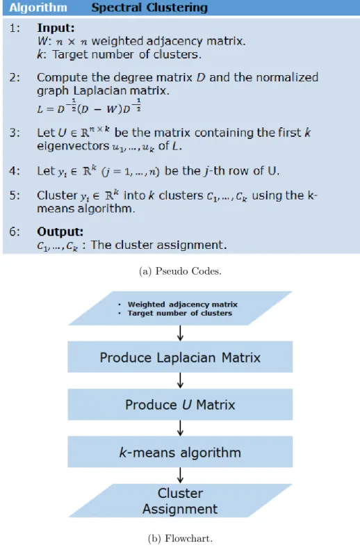
2.3 Spectral Clustering Algorithm. . . 13
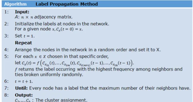
2.4 Pseudo Codes for Label Propagation Methods. . . 14
3.1 LabelRank Algorithm. . . 19
3.2 Modularity Change by Iterations in Real Graphs. . . 20
3.3 Modularity Change by Iterations in Simulated Graphs. . . 21
3.4 LabelMod Algorithm.. . . 23
3.5 Probability Matrix Used in Simulation Graphs . . . 26
3.6 Performance Time Comparison. . . 29
3.7 Zachary’s Karate Club Network Example. . . 31
4.1 LabelMod Algorithm in Multi-layer Networks. . . 34
4.2 Spectral Clustering Algorithm in Multi-layer Networks. . . 35
4.3 Performance Time Comparison . . . 39
4.4 Random Index by the Selection of Community Number . . . 41
4.5 Random Index of Individual Layers and Layers Combined. . . 43
4.6 Purity of Individual Layers and Layers Combined. . . 43
4.7 Normalized Mutual Information of Individual Layers and Layers Com-bined. . . 44
4.8 Modularity of Individual Layers and Layers Combined. . . 44
4.9 RI, PUR, NMI, and MOD in One of Individual Layers and Layers Com-bined. . . 45
Figure Page
4.10 Modularity with Different r Values. . . 46
4.11 Modularity by Changing Parameter in. . . 47
ABBREVIATIONS
AIC Akaike Information Criterion
BIC Bayesian Information Criterion
LM LabelMod
LPA Label Propagation Method
MCL Markov Cluster Algorithm
MOD Modularity
NMI Normalized Mutual Information
PUR Purity
RI Random Index
SBM Stochastic Block Model
SC-GEN Spectral Clustering with Generalized Eigen-Decomposition
SC-SR Spectral Regularization
SC-ML Spectral Clustering in Multi-layer Network
NOMENCLATURE A Adjacency Matrix C Community Assignments H Entropy I Mutual Information in Inflation Parameter L Laplacian Matrix P Probability Matrix Q Modularity Function r Cut-off Parameter s Score Function
U Matrix Containing the First k Eigenvectors of u1, ..., uk
W Weighted Adjacency Matrix
ABSTRACT
Bang, Seokhun MSIE, Purdue University, December 2015. Community Detection Using Efficient Modularity Optimization Method: LabelMod with Single and Multi-layer Graphs. Major Professor: Seokcheon Lee.
Graph clustering is a field of study that helps reveal characteristics of commu-nities. Systems can be viewed as networks and form communities in various areas such as biology, computer science, engineering, economics, and politics. A clustering algorithm is a tool that detects communities and it can be also considered as a pre-processing step to study the characteristics of detected communities. Many efforts were made to develop a well performing clustering algorithm in different types of net-works. In recent literature, a concept of multi-layer graphs emerged, and clustering algorithms are being developed to detect communities in the multi-layer graphs. In this thesis, we propose a clustering algorithm that can be applied to both single-layer and multi-layer graphs. We test the algorithm on simulated data and real data in both single-layer and multi-layer graphs. Four performance measures were used to evaluate the performance of the proposed algorithm. We also study how the performance mea-sures are correlated with each other and what the effects of parameter, presented in the proposed algorithm are. The thesis concludes with summary of research findings and directions of the future research.
1. INTRODUCTION
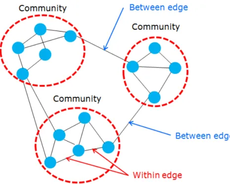
A network consists of nodes and edges. In a network, a node represents an individual identity and an edge is a connection between nodes. In most cases, systems can be viewed as networks, and this is the reason why people make efforts to analyze networks. Graph clustering is a field of study that helps to reveal characteristics of networks by identifying communities, and clustering algorithms are the tools to detect communities. Fortunato [1] also defines communities as groups of individuals that share common properties and have similar roles in the network. The objective of graph clustering is to detect community structure based on the edge connections. It does not focus on what the common properties in the same group are. Common properties are usually analyzed after communities are found. Therefore, graph clustering can be considered as a pre-processing step in understanding the characteristics of a network. Utilizing a suitable clustering algorithm will result in the detection of distinct communities and increase the probability of features that each community has. One of the most powerful quality functions, modularity, evaluates clustering results regard-ing the density. The density of communities is affected by the number of between edges and within edges. Between edges are connections between nodes in different communities. Within edges connect nodes in the same community. The modularity function that was proposed by Newman et al. [2] is shown in Equation 1.1:
Q= 1
2m
X
ij
(Aij −Pij)δ(Ci, Cj) (1.1)
In Equation 1.1, m is the total number of edges of the graph, A is the adjacency
matrix, andP is the edge probability between nodeiand nodej. δis a function that
has a value of 1 if node iand node j are in the same community, and 0 otherwise. In
Figure 1.1. Example of Graph Clustering
between edge or a within edge. The modularity equation only sums (Aij−Pij) values
with between edges. Modularity will be discussed again in Chapter 3 of this thesis. One of the most critical assumptions in graph clustering is that the graphs are not random. The purpose of graph clustering is to detect communities with common properties. If graphs are random, nodes will not have common properties, and no relevance is expected from having community.
In this thesis, several assumptions in the course of developing community detection are made as follows:
• Adjacency matrix can be either weighted or unweighted.
• Edges are undirected.
1.1 Problem Domain
There are many areas for which the associated system can be expressed as a network. Social network analysis had been already popular back in the 1930s and became one of the most important issues in sociology [3, 4]. Today, social network analysis has been expanded to social network systems such as Facebook or Twitter. These online platforms help people to communicate with others by allowing such services as messaging or photo sharing. Scholars have been researching about social groups’ behaviors, and clustering algorithms were used as a pre-processing step [5]. Online retailers like Amazon already use the clusters of customers of similar interest, as a target marketing technique to recommend other items for their clients [6].
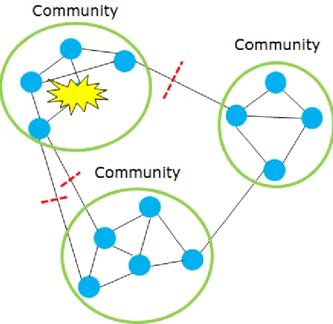
Graph clustering is also employed in the field of biology. In proteprotein in-teraction networks, proteins in the same community might provide similar functions within the cell [7–11]. Graph clustering can be also applied to protect from dangerous diseases that spread between humans. Figure 1.2 is an illustration of when disease occurs. Although there are several conditions that disease can transfer, disease spread by humans can be controlled by disconnecting between edges. Furthermore, a pre-dictive model can be developed to determine which groups have higher risk of disease infection and pose the most risk of damage to a society.
1.2 Research Objectives
In graph clustering problems, the algorithms cannot always identify communities perfectly because they only consider node and edge information in the network. More-over, most of the graph clustering problems are difficult and time-consuming to solve regarding maximizing modularity. Therefore, developing a effective and time-efficient clustering algorithm is critical.
A protein-protein interaction network is an example where the proteins’ ground truth community information is unknown. In this case, accuracy cannot be measured, and instead, modularity is used. Higher modularity tends to have higher accuracy,
Figure 1.2. Graph Clustering Application in Disease Control
but this is not always true. There is no research about the conditions where high mod-ularity guarantees high accuracy; the relationship between modmod-ularity and accuracy should be studied further.
Most of the currently developed algorithms are only applied to a traditional net-work. However, a new concept of multi-layer networks has recently emerged [12]. Multi-layer networks are graphs that have multiple slices of individual networks that have the same nodes but different edges. Like multi-layer networks, graphs can have different characteristics.
Some networks can be dense, while other networks are sparse. It will be the best practice to categorize types and find the best-performing algorithms by types of networks. However, there is no network categorization as of yet, and it is very difficult
to prove that one clustering algorithm outperforms another. Therefore, by finding a generalized clustering algorithm that guarantees a satisfactory result is beneficial. There are numerous algorithms, but the theorems and mathematical proof bases are weak [1]. By developing a new clustering algorithm, we hope that our new algorithm can contribute to the findings of new theorems and mathematical proof of graph clustering. Below, there are three main objectives of our research:
• Develop a well-performing and time-efficient clustering algorithm.
• Develop a clustering algorithm that guarantees not only high modularity but
also accurate clustering results.
• Develop a generalized clustering algorithm that performs well on different types
of network.
1.3 Organization of the Thesis
In Chapter 1, we briefly looked at what graph clustering is. We also discussed its applications and three main objectives of this research. In the next chapter, we look into the related literature about well-known existing algorithms, discuss a recent concept of multi-layer networks, and study several algorithms that are essential to our algorithm. In Chapter 3, we present how our methods are developed and how they perform in a single-layer network. In Chapter 4, our method is applied to multi-layer networks by simply aggregating individual single-layer networks. In the last section, Chapter 5, we conclude the thesis with our results and provide suggestions for future research.
2. LITERATURE REVIEW
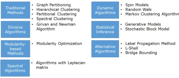
Graph clustering does not have a long history compared with graph theory. The idea of graph theory first emerged in 1736 and was originated by Euler [13]. On the other hand, the idea of graph clustering became famous in the early 21st century. Newman and Girvan were the pioneers of this field who used graph clustering methods in the network [14, 15]. After the emergence of graph clustering, it is now applied to various fields like sociology [3–5], marketing [6], biology [7–11], and many more [16–18]. Even with a brief history, numerous algorithms were developed and tested. Fortunato surveyed existing algorithms and organized algorithms into seven categories [1].
In this chapter, we will survey the literature. First, various algorithms in graph clustering will be presented. We explain how algorithms work and how algorithms in several categories differ. Then, we discuss multi-layer networks, which constitute one of the types of network. An investigation about using spectral methods will follow. The chapter will conclude with a literature survey on label propagation methods.
2.1 Existing Algorithms
The first category of clustering algorithms is referred as traditional methods. Graph partitioning, hierarchical clustering, partitional clustering, and spectral clus-tering are known traditional methods. These algorithms were already used in dif-ferent fields for difdif-ferent purposes. The Kernighan-Lin algorithm is one of earliest graph partitioning method that was proposed in the 1970s [19]. The algorithm was first developed to solve electric circuit partitioning. Hierarchical clustering has two approaches: The first is agglomerative algorithms where communities are created by merging each iteration. The second approach is divisive hierarchical algorithms where communities break down in each iteration. Agglomerative hierarchical
algo-Figure 2.1. Categories of Clustering Algorithms.
rithms cluster from bottom to top while divisive hierarchical algorithms function in
a top to bottom manner. In partitional clustering, k-means clustering is most often
used [20]. Numerous authors have proposed an extended version of k-means
cluster-ing [21–23]. Spectral clustercluster-ing is very similar to the partitional clustercluster-ing method except that it uses elements of the eigenvector to derive features based on nodes and
edges; then the algorithm computes a k-means clustering [24, 25]. Most of the
tradi-tional methods are limited due to their need for prior information. The number of communities should be predefined except for hierarchical clustering.
The second category is divisive algorithms. The main concept of divisive algo-rithms is to detect the between edges and remove them until no between edges exist. Divisive algorithms are very similar to divisive hierarchical clustering. However, di-visive algorithms remove between edges rather than removing low similarity edges between pairs of nodes. The algorithm of Girvan and Newman is considered to be the start of the divisive algorithm in graph clustering [2, 14, 15]. The algorithm com-putes the centrality for all edges and removes the edge with the largest centrality. When there is a tie, one is randomly chosen. The algorithm iterates until it cannot find any between edge. Since the time when Girvan and Newman were the pioneers
of graph clustering, other authors have proposed variants of this algorithm [9, 23, 26]. The weakness of this algorithm is that it cannot find clusters in overlapping commu-nities. Developing an algorithm that can deal with the overlapping communities is one of the rising research topics in this field.
The third category is modularity-based methods. Modularity is a quality function that was first proposed by Girvan and Newman, which was originally used to deter-mine the stopping criterion of their algorithm [14]. Now, considered one of the most important methods of defining good clusterings. There are efforts to utilize this mod-ularity function in the algorithm. In graph clustering, some algorithms that do not use a modularity function are fast but resulted in poor clusters [27–29]. Applying a modularity function has an advantage of higher probability to produce more accurate clusterings, but it may also increase the computational complexity [30–32]. Some al-gorithms [33–35] were developed to have both reasonable computational complexities and satisfactory accuracies.
Another category of clustering algorithms is spectral algorithms. Spectral clus-tering was already introduced as divisive algorithms; this category is different from the divisive algorithms but shares a similar concept. Like spectral clustering, spec-tral algorithms compute eigenvectors from a Laplacian matrix. However, instead of
using k-means clusterings at the end, spectral algorithms use different methods. An
algorithm that was proposed by Capocci et al. [36] uses eigenvector values of the right stochastic matrix where the matrix is computed from the adjacency matrix by
dividing number of edges in node i.
Spin models are methods in dynamic algorithm categorization that consider a
system of spins in q different states. One of the most well-known models is the Potts
model [37]. Based on the Potts model, Blatt et al. [38] and Reichardt et al. [39] developed the spin model further. Another method in a dynamic algorithm is a random walk model [40]. A random walker would remain longer in a community due to the characteristics of the networks that a denser network tends to have more within edges than between edges. Zhou has developed several algorithms using the random
walk [41]. Zhou first developed an algorithm by using a distance between nodes by employing a random walk. In the next paper, Zhou measured the dissimilarity of nodes by using random walk distance [42].
Van Dogen [43] developed the Markov Cluster Algorithm (MCL). This algorithm first computes a probability matrix and it subsequently continues iterative steps of expansion and inflation until a steady state is reached. In MCL, expansion is a matrix
multiplication process with the power of e. Inflation uses the following equation:
(ΓrM)pq = (Mpq)r/
k
X
i=1
(Miq)r (2.1)
Here, M is a stochastic matrix such that a value in row i and column j is the
probability of going from node j to node i. There is an inflation parameter,r, which
is always greater than 1. An inflation operator works like a normalization process in that if the nodes have similarity regarding the random walk distance, the value in the matrix will increase. In the opposite case, if the nodes have dissimilarity, the value will decrease. MCL and its inflation operator will be discussed again later in Chapter 3.
Statistical inference is another category in which the method starts with a set of observations and decides a hypothesis of a model. Two famous models in statistical inference methods are generative models and block modeling. A generative model
uses Bayes’ theorem and it has an aim to find a parameter {θ} that maximizes the
posterior distribution below:
P({θ}|D) = R P(D|{θ})P({θ})
P(D|{θ})P({θ})dθ (2.2)
Here, P({θ}) is the prior distribution and D is the information about the system.
The problem of the generative model and of using Bayesian inference is the fact that the equation includes the integral. Having an integral in the equation will result in more computational complexity. Also, the choice of the prior distribution is not clear as well. Some researchers tried to apply this model in social networks [44–46] and biological networks [47, 48].
Another well-known statistical approach is block modeling. Block modeling finds a group of nodes with similar characteristics. Nodes form a community by two types of equivalence: structural equivalence [49] where nodes have same neighbors and regular equivalence [50] where nodes have similar patterns of connection. As an extension, the Stochastic Block Model [51] uses a stochastic equivalence that is analogous to the structural equivalence where similar linking probabilities are considered to be of the same class. Because a statistical inference method is model-based rather than algorithm-based, it is important to select a model that suits the data well. Common statistical model selection heuristics include the Akaike Information Criterion (AIC) [52] and the Bayesian Information Criterion (BIC) [53].
Sometimes, communities are detected by using the information theory. However, a deeper review of information theory is out of our research scope. Mutual information [54] is a measure that informs about how much one solution is learned when the other solution is known. Mutual information can be computed by subtracting a conditional entropy of two clustering results from a marginal entropy of one clustering result. The equation for mutual information is as follows [1]:
I(X, Y) =H(X)−H(X|Y) =X x P(x)log 1 P(x) − X xy P(x, y)log 1 P(x|y) =X x X y P(x, y)log P(x, y) P(x)P(y) (2.3)
In the equation, H(X) is the marginal entropy of clustering assignment X and
H(X|Y) is the conditional entropy of X and Y. Both marginal entropy and
condi-tional entropy can be computed by utilizing marginal probability of x, joint
proba-bility of x and y, and conditional probability of x and y.
The last category, alternative algorithms, includes all of the algorithms that are not classified in previous categories. Methods like L-shell [55], Bridge Bounding [56] and other heuristic algorithms are in this category. The Label Propagation method
[57] is also an alternative algorithm. However, it will be discussed in more detail in Section 2.4.
2.2 Multi-layer Networks
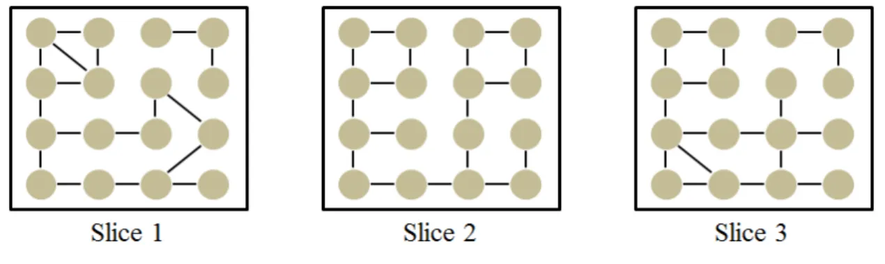
Mucha et al. developed a new framework of community structure named multi-slice networks [12]. By its definition, multi-slices of networks can represent variations over time, or different connections at various scales. Figure 2.2 is an example of multi-slice networks. In each multi-slice, the nodes are the same. However, the edges connecting the nodes are different across the slices. Mucha et al. used 110 slices of vote simi-larities [12]. They also used four slices of Facebook friendships, picture friendships, roommates, and housing groups on the ”Tastes, Ties, and Time” network [58].
Figure 2.2. Example of Multislice Networks.
After the emergence of the multislice concept, there were several efforts to ap-ply clustering algorithms in multi-layers of graphs. Dong et al. first developed two
methods, clustering with generalized eigen-decomposition (SC-GED) and spectral
regularization (SC-SR) [4]. Then Dong extended their algorithm (SC-ML) by using
the modified Laplacian matrix Lmod [10]. SC-ML outperformed its competing
algo-rithms in purity, normalized mutual information, and random index. In addition to Dong’s work, Zhang et al. used the multi-layer graph concept in gene co-expression
networks [59]. Hu et al. also applied the multislice concept in optimizing modu-larity [60]. In their study, clustering results were used as an image segmentation. The pixels in the image functioned as an adjacency matrix. However, due to a large number of pixels, it required a considerable amount of memory and had an expensive computational time. The authors also pointed out in their paper that a computational improvement is required to deal with an increased amount of network data.
2.3 Spectral Clustering
As briefly explained in the previous section, spectral clustering is an algorithm that uses an eigenvector decomposition of a Laplacian matrix. Then the algorithm runs a k-means clustering algorithm by using few major eigenvectors. The more detailed
procedure is shown in Figure 2.3. By combining a spectral method with k-means
clustering, it became one of the most well-known algorithms for graph clustering. Some researchers used a spectral clustering in multi-layer graphs [4, 10, 59]. However,
selecting an appropriate k value is another problem in spectral clustering. When
ground truth communities are known, the algorithm can use the number of ground
truth communities as k. On the other hand when ground truth communities are not
known, the selection of k is vague. Pham et al. provided a guideline on howk should
be selected in k-means clustering [61]. In our research, spectral clustering is one of
(a) Pseudo Codes.
(b) Flowchart.
2.4 Label Propagation Method
The Label Propagation Method (LPA) was first proposed by Raghavan et al. to be used in a large-scale network graph clustering [57]. The algorithm starts with independent labels. At every step, nodes look for their neighbors’ labels and change their label with the maximum occurring labels. When there are ties among neigh-bors, labels are assigned uniformly and randomly from the neighbors. The algorithm continues the iterative process until there are no label changes in the network. After finishing this iterative process, nodes with same labels are considered to be in the same community.
The algorithm was first proposed in a non-overlapping community situation where nodes can have only one community assignment. However, more research was con-ducted to solve a clustering problem in overlapping communities [62–64] Xie et al. improved both computational efficiency and the quality of clustering by proposing a new update rule and label propagation criterion [65]. Figure 2.4 present a detailed procedure of how the algorithms work.
Despite the fact that LPA has a significant advantage of performing in a near-linear time to run the algorithm, LPA has several disadvantages. First, LPA has a convergence issue. The network that is bipartite or a nearly bipartite will cause oscillations of labels and will not form clusters. To deal with this challenge, Raghavan et al. suggests using an asynchronous update instead of a synchronous update. In a synchronous update, the algorithm only considers previous iterations labels of a nodes neighbors. On the other hand in an asynchronous update, the algorithm considers neighbors labels that were updated in both current and previous iterations. By using an asynchronous update, the algorithm can have a wider range of labels and can use both past and present information of the labels.
The second disadvantage and the most critical drawback is the randomness issue. Because this algorithm uses an asynchronous update, the sequence of the update differs by runs and the tie breaker using uniform random selection aggravates the diffusion of results. Raghavan et al. suggested using an aggregation of solutions [57].
However, Tib`ely et al. showed that the aggregation method would fragment the
communities into several pieces [66]. Even with an effort to resolve the randomness of LPA solutions, there has been no satisfactory extension to date.
3. LABELMOD IN SINGLE-LAYER GRAPHS
In this chapter, we will discuss LPA further as well as its inherited algorithm La-belRank. First, the LabelRank algorithm will be explained because our proposed algorithm follows similar steps. Then, the proposed algorithm will be described in more details. Later in this chapter, the proposed algorithm will be applied to both simulated data and real data in a single-layer graph. The proposed algorithm’s per-formance will be compared with other algorithms.
3.1 LabelRank Algorithm
In Chapter 2, the literature survey described what LPA is. In summary, LPA is a heuristic algorithm that propagates a node’s label to its neighbors. Because it does not utilize matrix operation in the algorithm, the algorithm is fast and efficient. However, to solve the label’s oscillation problem, the algorithm randomly starts at each iteration and updates asynchronously. Because of the algorithm’s characteristics, LPA produces different clustering results. Xie et al. have proposed an algorithm named LabelRank to resolve this kind of random clustering result that characterizes LPA [67].
LabelRank is similar to the Markov Cluster Algorithm (MCL) while it keeps the properties of LPA. MCL is based on the simulation of random walks that use two op-erators, expansion, and inflation. Two operators continue until there are no changes in the probability matrix [68]. LabelRank resembles MCL in using an inflation op-erator. Also, both algorithms pursue the process of controlling and normalizing a matrix. However, the most significant difference between the two algorithms is that LabelRank utilizes the label distribution matrix that normalizes after each iteration while MCL uses probability matrix to normalize. LabelRank retains the advantages
of fast and efficient characteristics of the LPA. The modularity of LabelRank was at least similar or even better than its predecessor algorithms, LPA, and MCL. However, there were questionable parts of the algorithm that needed to be improved.
The algorithm that we are proposing is similar to the LabelRank algorithm by Xie et al. The main idea of LabelRank is to perform iterative steps of propagation and normalization in the network. Although there are two key steps, the algorithm consists of four operators: 1) propagation, 2) inflation, 3) cut-off, and 4) conditional update. LabelRank maintains different labels throughout the process and nodes with the highest probability label at the end of the algorithm form a community. Since all processes are operations of a matrix, there is no randomness issue. Indeed, the algorithm is synchronous, and it does not have the problem of label oscillations even in a bipartite network. The following are detailed descriptions of the algorithm:
1)Propagation: With a given adjacency matrix ofA(n ×nmatrix whose entries are 1 if there are edges connected between nodes and 0 otherwise), it is possible to
compute a label distribution matrix ofP (n×n matrix that assigns equal probability
on nodes that have edges). The label distribution matrix can be obtained by the following equation:
Pij =
1 ki
, ∀j s.t. Aij = 1 (3.1)
Once the label distribution matrix is created, it can be updated by matrix mul-tiplication with the adjacency matrix. The propagation operator can be applied by the following equation:
2) Inflation: The inflation operator concept originally came from the MCL. In MCL, the inflation operator works for the stochastic matrix while the label distribu-tion matrix is applied in LabelRank [67].
P00 = ΓinP 0 = (P0)in/ n X j=1 (P0)in (3.3)
There is one parameter, in, that controls the inflation. If two nodes are strongly
connected, the operator will increase the probability. On the other hand, the operator will decrease the probability if two nodes are weakly connected. After iteration, the value in the matrix will likely be close to 0 or 1.
3) Cut-off: After the inflation operator, there could be small probabilities in the label distribution matrix. These low probabilities will eventually merge to zero after iteration. Both the inflation operator and the cut-off operator are key hard thresholding steps of the algorithm.
4) Explicit Conditional Update: Xie et al. mentioned that well-clustered communities can be detected far before the convergence [67]. Therefore a conditional update operator helps to find the best solution before the convergence. The node gets updated only when there are significant differences. A detailed update condition is the following:
X
j∈N b(i)
isSubset(Ci∗, Cj∗)≤qki (3.4)
Here, Ci∗ is the maximum label set with the maximum probability at nodeiat the
previous iteration and the function isSubset compares with its neighbors maximum
labels. If Ci∗ ⊆ Cj∗, the function returns 1 and it returns 0 if Ci∗ is not a subset of
Cj∗. There are parameter q ∈ [0,1] and ki the degree of node i to make a condition
whether or not to change the labels.
The algorithm continues iterative steps of four operators until there are no changes in the node labels. Once the iterative steps are completed, the algorithm detects a community membership of each node with a certain probability. The most significant
strength of this algorithm is that it keeps the concepts of both LPA and MCL while the randomness issue is eliminated.
(a) Pseudo Codes.
(b) Flowchart.
3.2 Algorithm Development
In the conditional update operator of the original LabelRank algorithm, a node’s label changes whenever the conditional update statement is satisfied. However, when the algorithm was tested, we found that the conditional update will be greatly
de-pendent on the parameter q. None of the literature papers mention this conditional
update, and the reason for utilizing a conditional update operator was not sufficient. However, we found that the previous three operators are easy to implement and have fast performance. Therefore, we analyzed the LabelRank algorithm to determine its significant characteristics and developed an algorithm by introducing a new condi-tional update and stopping criterion.
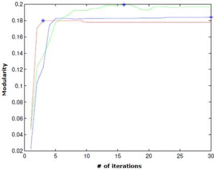
Different color indicates different networks.
Figure 3.2. Modularity Change by Iterations in Real Graphs.
Figures 3.2 and 3.3 are plots of modularity changes over 30 iterations. A blue asterisk (*) is a maximum modularity among 30 iterations. A modularity reaches the maximum and then stabilizes in Figure 3.2. Often, modularity oscillates, but the oscillation stabilizes within five iterations. On the other hand, a modularity
Different color indicates different runs.
Figure 3.3. Modularity Change by Iterations in Simulated Graphs.
value reaches its maximum and suddenly decreases in Figure 3.3. By inspecting both figures, modularity reaches its maximum and then its value will either decrease or stabilize.
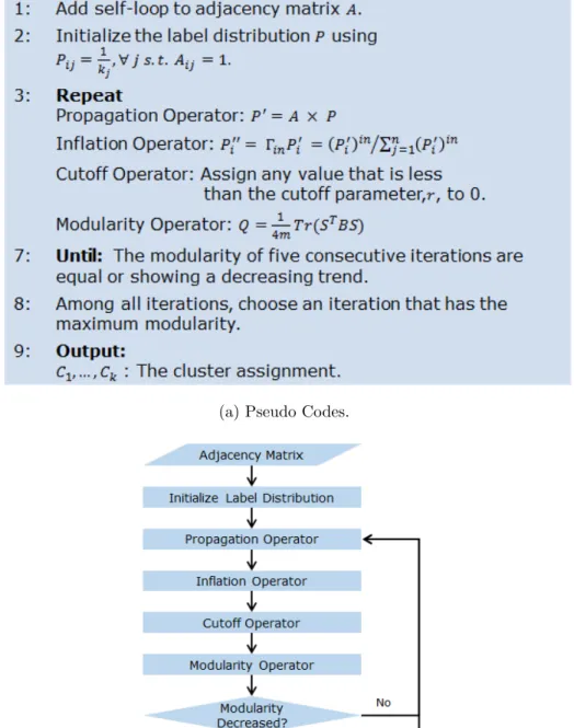
Our proposed algorithm, LabelMod, utilizes the fact that a modularity either decreases or stabilizes when the iteration increases in LabelRank. LabelMod keeps propagation, inflation, and cut-off operators and includes the modularity operator instead of the conditional update operator. The modularity operator works in each iteration and evaluates whether the algorithm should stop or continue to the next iteration. Among several equations of modularity proposed by different authors, we use the following equation [69]:
Q= 1
4mT r(S
TBS) (3.5)
In this equation,mis the total number of edges in the network. Sis the non-square
B is the modularity matrix where B = A− kikj
2m. LabelMod’s modularity operator
compares previous modularity with current modularity to check if it decreased. If modularity values are having a stabilizing or decreasing pattern for five iterations, the algorithm stops and selects a maximum modularity among iterations.
This stopping criterion is intuitive but powerful. It does not guarantee a global maximum modularity value. However, it guarantees a local maximum modularity value. Mathematical programming techniques would find a global maximum value, but then, the computational cost would be very expensive and cannot be considered as a suitable algorithm. There is always a tradeoff in which accuracy requires more time to be spent. LabelMod is an algorithm that balance both accuracy and computational time. Because of its balanced nature, it can be applied to any type of network even with no priori information.
(a) Pseudo Codes.
(b) Flowchart.
3.3 Results
In our research, LabelMod algorithm was applied to 1) simulated graphs, and 2) real graphs. In this section, LabelMod’s performance will be compared with Spectral Clustering (SPC) which is one of the most well-known algorithms, and the Label Propagation (LPA) Method. For the algorithms’ performance comparison, random index (RI) [70], purity (PUR), normalized mutual information (NMI) [71], and mod-ularity were measured. For both the simulated graphs and the real graphs, ground truth communities were given.
The first performance measure, random index, is an accuracy measure based on a binary decision. After communities are detected, random index compares each node’s community assignment with the ground truth community.
RI(Ω, C) = T P +T N
T P +F P +F N +T N (3.6)
Here, TP, TN, FP, and FN stand for true positive, true negative, false positive, and false negative. Ω represent communities found by the algorithm and C represent ground truth communities. By summing true positive and true negative values, the equation counts how many nodes are correctly assigned to the same community and correctly assigned to different communities. The counted value then is divided by the sum of total possibilities. Random index values range from 0 to 1 and are expressed in decimals.
Purity is another performance measure. It finds a maximum intersection between the algorithm’s community and ground truth community. Then it sums all of the algorithm’s communities and divides by the total number of nodes. The equation for the purity is as follows:
P urity(Ω, C) = 1 N
X
k
maxj|ωk∩Cj| (3.7)
Purity can be also considered as one of the accuracy measures, but, it also has one significant problem. Even in the case where the algorithm produces more com-munities than the ground truth comcom-munities, purity can be 1. Smaller comcom-munities
can be aggregated together to form a ground truth community. Purity is not a useful measure if one wants to find an exact clustering with equal community sizes as the ground truth. However, purity is useful in clustering in overlapping communities or hierarchical structures.
The last performance measure is normalized mutual information. NMI uses mu-tual information between the algorithm community and ground truth community. Then it is normalized using the entropy of clusters. There are many different ways to normalize mutual information; we used the following equation [72]:
N M I(Ω, C) = I(Ω;C)
[H(Ω) +H(C)]/2 (3.8)
Mutual information measures the information that two clustering results share.
Here,I(Ω;C) refers to the mutual information andH(Ω) orH(C) refer to the entropy.
Mutual information and entropy can be computed by using the equations below:
H(Ω) =− R X i=1 ai Nlog ai N (3.9) I(Ω;C) = R X i=1 C X j=1 nij N log nij/N aibj/N2 (3.10)
N is the total number of nodes, and nij is the number of nodes that are common
between the algorithm’s community and the ground truth community. ai is Pinij
and bj is
P
jnij.
By using three performance measures together, three algorithms can be compared objectively. Along with three performance measures, modularity was calculated for the three algorithms as well. Since LabelMod has a modularity operator inside its algorithm, it is expected that LabelMod will have higher modularity most of the time.
3.3.1 Graph Simulation
In graph clustering, the Stochastic Block Model (SBM) can generate a random net-work by assigning each node with a ground truth community [73]. First, a probability
matrix that will be used to construct the adjacency matrix is needed. A probability
matrix is an n × n matrix where n is the total number of communities. Diagonal
entries in the matrix are within community edge probability, and the rest are between community edge probability. An adjacency matrix can be produced by utilizing the probability matrix. Zhang et al. also used SBM to produce three communities with a given probability matrix as follows [59]:
Figure 3.5. Probability Matrix Used in Simulation Graphs
In their experiment, they had four different probability matrices with 50 runs and three communities in each run. This task was done with two different conditions; in one condition, an equal community size was used, and the other had a different com-munity size. The same experimental method was conducted to test the performance of LabelMod. When the community size was the same, the network had 50 nodes in each one community, and the network consisted of three communities. When the community size was different, the network had 30 nodes in two communities and 90 nodes in one. In simulated studies, we found that different community size networks have slightly lower performance measures with higher standard deviations. Table 3.1 includes random index, purity, normalized mutual information, modularity and per-formance time data with the same community size for four conditions and Table 3.2 includes the same performance measures but with different community size.
When the community size was the same, LabelMod produced high-performance measures. Compared with other algorithms it especially performed better in
normal-ized mutual information. Also, as expected, LabelMod’s modularity outperformed the other two algorithms’ modularity. However, the performance time was relatively higher than the other algorithms. The spectral clustering algorithm outperformed with respect to performance times; this was because it does not require many
compu-tations to calculate a Laplacian matrix. Nevertheless, it uses k-means clustering that
is one of the most popular algorithms in the field. Although spectral clustering was
the fastest, it did not always produced a satisfactory result. In the P1 matrix, there
is no between edge probability. In this case, spectral clustering failed many times. When no between community edge exists, an eigenvector decomposition produces an
empty Laplacian matrix that causes a failure in k-means clustering.
When the community size was different, the performance measure continued to decrease as more between community edges were produced. LabelMod still had the highest modularity at all times, but the spectral clustering maintained its perfor-mance. Spectral clustering’s performance time was the fastest and LabelMod was the slowest-performing algorithm in the experiment. However, when the network had more edges, the algorithm performed faster. The performance time is highly related to the total number of nodes rather than the total number of edges. Most of the computational time is spent in matrix operations. If the network has more nodes, the size of the matrix also increases and causes an expensive computational cost. On the other hand, when there are more edges in the network, edges interact more actively in the inflation step.
T able 3.1: Sim ul ated Graphs Result (Same Comm unit y Size) P1 P2 P3 P4 SPC LP A LM SPC LP A LM SPC LP A LM SPC LP A LM RI 0.92 (0.12) 0.85 (0.07) 0.99 (0.01) 0.92 (0.14) 0.83 (0.07) 0.99 (0.02) 0.91 (0.14) 0.83 (0.06) 0.97 (0.04) 0.91 (0.14) 0.82 (0.11) 0.93 (0.08) PUR 0.89 (0.16) 1 (0) 1 (0) 0.89 (0.16) 0.98 (0.01) 0.99 (0) 0.88 (0.17) 0.96 (0.03) 0.98 (0.02) 0.88 (0.17) 0.91 (0.12) 0.95 (0.05) NMI 0.89 (0.15) 0.71 (0.10) 0.98 (0.03) 0.87 (0.18) 0.66 (0.10) 0.96 (0.05) 0.84 (0.19) 0.62 (0.11) 0.89 (0.11) 0.81 (0.21) 0.61 (0.16) 0.80 (0.16) Mo dularit y 0.2492 (0.04) 0.2579 (0.23) 0.3071 (0) 0.2336 (0.04) 0.2358 (0.03) 0.2859 (0) 0.2167 (0.04) 0.2235 (0.02) 0.2627 (0.01) 0.2045 (0.04) 0.2082 (0.03) 0.2399 (0.02) Time 0.06s (0.02s) 1.01s (0.34s) 1.04s (0.22s) 0.08s (0.02s) 0.94s (0.29s) 1.06s (0.16s) 0.08s (0.02s) 1.03s (0.25s) 1.04s (0.13s) 0.09s (0.03s) 1.14s (0.36s) 1.15s (0.25s) SPC: Sp ectral Clustering / LP A: Lab el Propagation Metho d / LM: Lab elMo d T able 3.2: Sim u lated Graphs Result (Differen t Comm unit y Size) P1 P2 P3 P4 SPC LP A LM SPC LP A LM SPC LP A LM SPC LP A LM RI 0.88 (0.14) 0.90 (0.02) 0.94 (0.06) 0.83 (0.17) 0.89 (0.05) 0.88 (0.05) 0.89 (0.10) 0.76 (0.15) 0.86 (0.04) 0.89 (0.11) 0.55 (0.19) 0.85 (0.04) PUR 0.89 (0.10) 1 (0) 1 (0) 0.83 (0.11) 0.98 (0.01) 0.98 (0.1) 0.85 (0.10) 0.91 (0.07) 0.97 (0.01) 0.86 (0.08) 0.78 (0.11) 0.96 (0.02) NMI 0.83 (0.17) 0.74 (0.02) 0.84(0.11) 0.63 (0.24) 0.69 (0.05) 0.69 (0.09) 0.69 (0.16) 0.56 (0.11) 0.63 (0.06) 0.67 (0.15) 0.37 (0.16) 0.59 (0.06) Mo dularit y 0.1574 (0.03) 0.1590 (0.01) 0.1766 (0) 0.1354 (0.03) 0.1518 (0.01) 0.1618 (0.01) 0.1400 (0.02) 0.1291 (0.02) 0.1516 (0.01) 0.1414 (0.02) 0.0900 (0.03) 0.1479 (0.01) Time 0.07s (0.02s) 0.77s (0.20s) 1.15s (0.30s) 0.08s (0.02s) 0.71s (0.18s) 0.77s (0.11s) 0.08s (0.02s) 0.83s (0.23s) 0.73s (0.10s) 0.08s (0.02s) 0.96s (0.25s) 0.70s (0.08s) SPC: Sp ectral Clustering / LP A: Lab el Propagation Metho d / LM: Lab elMo d
Both Table 3.1 and Table 3.2 show that the standard deviation of LabelMod is much smaller than the rest. The algorithm produces stable clustering results. These results also imply that LabelMod will still produce a solid clustering result whether the network is sparse or dense. This stability is one of LabelMod’s advantages that makes the algorithm fascinating even with a slower performance time. With the same graph, the label propagation method produces stochastic results. Raghavan et al., who proposed this algorithm also suggest using an aggregation method to deal with the stochastic results [57]. Although the aggregation method is not complex, the user should run it several times before aggregating which requires multiple computational times.
It is true that random results can sometimes be better than deterministic results. However, the performance time is one of the most important issues since graph clus-tering is more like a pre-processing step for further analysis. Therefore, algorithms cannot be tested an infinite number of times, and deterministic results are preferred.
In addition, algorithms were tested with a larger number of nodes. Performance time was measured using MATLAB with Intel(R) Core (TM) i5-3337U CPU @ 1.80GHz processor that has 4 GB of RAM. Figure 3.6 is a plot comparing a number of nodes to the performance time. Both LabelMod’s result and spectral clustering’s re-sult show exponential shapes of a curve; however, LabelMod’s performance time was worse. The gap of performance time is due to the coding that is not optimized. The label propagation method shows a linear line because the algorithm is not affected by the number of the nodes. The computational complexity of LabelMod [74, 75] and
spectral clustering [76] are O(n2) while the label propagation method is O(m) where
m is the number of total edges [57]. The label propagation method is expected to
have better performance in a sparse network. However, the algorithm will have a significant performance disadvantage in a dense network.
3.3.2 Real Graphs
In graph clustering, there are real graphs where the ground truth communities are known. In this section, LabelMod was tested in the real graphs in which the true communities are already known. The first network is called Zachary’s Karate Club
network1. In this network, nodes are 34 members of the club and edges are their
friendship status [77]. This club later has a conflict between the instructor and the president which are two ground truth communities.
The second network is the US College Football network where nodes are colleges and edges are produced by Division I games for the 2000 season. In the 2000 season, there were 115 colleges in 12 conferences. In this network, there are 12 ground truth communities [14].
The last network is the Dolphins network. A network of 62 bottlenose dolphins was observed over seven years. Edges were formed when two dolphins were paired
Figure 3.7. Zachary’s Karate Club Network Example.
more frequently than expected. The ground truth communities of this network were the sex groups that were equal to two [78].
Table 3.3: Real Graphs Result
Karate Football Dolphins
SPC LPA LM SPC LPA LM SPC LPA LM
RI 0.9265 0.9118 1 0.7312 0.9790 0.9790 0.5860 0.6989 0.6882
PUR 1 0.9706 1 0.3217 0.9304 0.9304 0.6613 0.7742 0.7097
NMI 0.8384 0.6861 1 0.5879 0.9269 0.9269 0.1240 0.2626 0.1391
Modularity 0.1524 0.1759 0.1796 0.1690 0.1828 0.1828 0.1647 0.1968 0.1992
Time 0.0469s 0.0625s 0.1250s 0.1406s 0.3281s 0.9844s 0.0938s 0.2813s 0.2500s
SPC: Spectral Clustering / LPA: Label Propagation Method / LM: LabelMod
The test result in Table 3.3 shows that LabelMod outperformed the other two algorithms in the Karate network. In contrast, LabelMod’s performances were
network in which community structure is weak, and the clustering performance for all algorithms is lower compared with the other two networks. As shown in our simulated graphs, LabelMod’s performance time was still higher than the other al-gorithms. However with a more dense network like the Dolphins network, LabelMod was faster than the label propagation methods. The performance time of LabelMod depends on the number of nodes, and a larger number of edges reduces LabelMod’s performance time. Both the real graph results show that each algorithm has both strengths and weaknesses. Spectral clustering usually performs well in non-sparse networks, and it performs better when a priori information on the number of ground truth communities is given. The label propagation method performed well for a short period, but it has disadvantages of producing different results with the same network. On the other hand, LabelMod automatically detects communities without having a priori information with a stable performance. Because LabelMod uses a modularity operator, it always produces higher modularity than other algorithms that do not use a modularity optimization.
Graph clustering is a field of study where both time and accuracy are important. If nodes cluster well, it can be utilized as a useful tool for further analyses like social behavior, target marketing or bioinformatics. Many algorithms are developed, and different approaches have been made for several years. It is difficult to prove which algorithm is superior; however, LabelMod is the algorithm that yields stable results within a reasonable performance time.
4. LABELMOD IN MULTI-LAYER GRAPHS
4.1 Algorithm Development
In this chapter, we propose a new integration concept with a LabelMod algorithm that was introduced in the previous chapter. Due to LabelMod’s characteristics that the algorithm can be applied to any network, it can be utilized in multi-layer graphs as well. It is common that most algorithms integrate results after finding nodes’ com-munity membership. However, our proposed algorithm aggregates graphs beforehand to make one weighted graph and process the actual clustering steps afterward. Adja-cency matrices in different layers can be simply added and produce a new weighted matrix that represents all layers. Then, a label distribution matrix can be made by summing each layers probability matrix multiplied by the score of the graph. The score of the graph is described as follows:
si =
Ei
PG
i=1Ei
(4.1)
Here, Ei is the total degree of edges and G is the total number of layers. Once
a weighted graph and a new propagation matrix have been created, LabelMod can be applied just like finding communities in a single layer network. The algorithm continues iterative steps of propagation operator, inflation operator, cut-off operator, and modularity operator until the stopping criterion is satisfied. The stopping crite-rion checks five consecutive modularity values for equality or for showing a decreasing trend.
(a) Pseudo Codes.
(b) Network Aggregation Example.
(a) Pseudo Codes.
(b) Flowchart.
4.2 Results
The algorithm was tested with experimental data that are similar to those in the previous chapter and synthetic gene co-expression data for performance comparison. The performance evaluation methods are the random index, purity, and normalized mutual information. Modularity was also compared to see if LabelMod’s modularity was higher than the comparison algorithm. The spectral clustering algorithm in multi-layer graphs [79] uses a modified Laplacian matrix instead of a regular Laplacian matrix by eigenvector decomposition. The rest of the algorithm follows similar rules
of the original spectral clustering algorithm. Parameter α plays a significant role in
the clustering results. Pseudo code for the spectral clustering algorithm in multi-layer graphs is provided above:
4.2.1 Graph Simulation
By using a Stochastic Block Model (SBM), an adjacency matrix was created based on four different probability matrices as in Chapter 3. Then this procedure was performed with 50 runs having three communities in each run. When the network was produced with equal community sizes, the network contained 50 nodes in each community. In the second condition where the network was made with different community sizes, two communities had 30 nodes, and one community had 90 nodes. Three layers of networks were produced.
T able 4.1: Sim ul ated Graphs Result (Same Comm unit y Size) P1 P2 P3 P4 SPC LM SPC LM SPC LM SPC LM RI 0.90 (0.13) 1 (0) 0.95 (0.11) 1 (0) 0.93 (0.12) 1 (0) 0.95 (0.11) 1 (0) PUR 0.88 (0.16) 1 (0) 0.93 (0.13) 1 (0) 0.91 (0.15) 1 (0) 0.93 (0.13) 1 (0) NMI 0.87 (0.17) 1 (0) 0.93 (0.14) 1 (0) 0.91 (0.15) 1 (0) 0.93 (0.14) 1 (0) Mo dularit y 0.2653 (0.06) 0.3079 (0) 0.2651 (0.05) 0.2872 (0) 0.2421 (0.05) 0.2683 (0) 0.2318 (0.04) 0.2510 (0) Time (s) 0.14 (0.03) 0.28 (0.05) 0.19 (0.03) 0.29 (0.05) 0.21 (0.03) 0.32 (0.06) 0.21 (0.03) 0.32 (0.06) SPC: Sp ectral Clustering / LM: Lab elMo d T able 4.2: Sim u lated Graphs Result (Differen t Comm unit y Size) P1 P2 P3 P4 SPC LM SPC LM SPC LM SPC LM RI 0.89 (0.12) 1 (0) 0.91 (0.12) 0.99 (0.02) 0.95 (0.10) 0.96 (0.04) 0.95 (0.10) 0.94 (0.04) PUR 0.91 (0.10) 1 (0) 0.93 (0.09) 1 (0) 0.95 (0.08) 0.99 (0.02) 0.96 (0.08) 0.98 (0.01) NMI 0.85 (0.17) 1 (0) 0.88 (0.16) 0.99 (0.05) 0.91 (0.08) 0.87 (0.12) 0.92 (0.13) 0.78 (0.10) Mo dularit y 0.1568 (0.03) 0.1780 (0) 0.1538 (0.03) 0.1705 (0) 0.1558 (0.02) 0.1509 (0.02) 0.1519 (0.02) 0.1368 (0.01) Time (s) 0.16 (0.03) 0.37 (0.08) 0.20 (0.03) 0.34 (0.07) 0.21 (0.03) 0.30 (0.08) 0.20 (0.03) 0.24 (0.04) SPC: Sp ectral Clustering / LM: Lab elMo d
When the community size was the same, LabelMod found a perfect clustering for all networks. All random index, purity, and normalized mutual information were 1. From this result, we found that LabelMod produces more accurate results when
networks are aggregated together. Modularity was also higher than the spectral
clustering algorithm in all networks. On the other hand, the spectral clustering
algorithm also produced strong performance measures, but the standard deviations for all measures were high. Most of its results formed an accurate clustering, but a poor clustering was occasionally made. The result has once again showed that LabelMod is an algorithm that produces stable clustering results. The performance time was still higher than spectral clustering’s performance time. However, the performance time gap between spectral clustering and LabelMod decreased. Since the spectral clustering algorithm in multi-layer graphs computes a Laplacian matrix of all layers, the performance time of LabelMod is much shorter than spectral clustering in a condition where numerous layers of graphs exist.
When the network had different community size, LabelMod’s performance did not outperform spectral clustering as in the experiment where the community size was the same. However, the performance was competitive with spectral clustering’s result.
Spectral clustering did not perform well in the P1 network because this P1 network
does not produce any between edges. LabelMod’s modularity value was always higher than spectral clustering in Table 4.1. However, spectral clusterings’ modularity values
were higher in P3 and P4 in Table 4.2.
Performance time was measured according to the total node sizes in networks with MATLAB. The performance time was tested with an Intel(R) Core (TM) i5-3337U CPU @ 1.80GHz processor that has a 4 GB of RAM. The test was conducted to see how LabelMod performs in an extensive network. In Figure 4.3, performance time for both algorithms is similar to the exponential distribution. However, LabelMod has a more acute angle of the slope.
The computational complexity of both algorithms isO(n2) which is due to then×n
the time gap still exist. However, LabelMod’s performance time can be potentially improved by coding with a sparse matrix function.
Figure 4.3. Performance Time Comparison
4.2.2 Gene Co-expression Graphs
A synthetic gene co-expression dataset was utilized to check the validation of LabelMod’s performances in multi-layer networks as in the previous research [59, 80]. The network was simulated with 50 conditions, and each gene was assigned to have one of 15 ground truth communities. Five samples were chosen, and three layers were included in each sample. A detailed description of constructing a gene co-expression network is as follows:
1. Pre-assign each node to one of 15 ground truth communities.
2. Compute Pearson’s correlation coefficient (Equation 4.2) with 50 conditions by each node.
3. If the absolute value of the Pearson’s correlation coefficient is larger than a
threshold parameter α, connect two nodes with an edge.
4. With given edge information, produce an adjacency matrix.
r = Pn i=1(xi−x)(y¯ i−y)¯ pPn i=1(xi−x)¯ 2 pPn i=1(yi−y)¯ 2 (4.2)
Table 4.3: Gene Co-expression Data Result
data0 data1 data2 data3 data4 SPC LM SPC LM SPC LM SPC LM SPC LM RI 0.9746 0.9866 0.9663 0.9850 0.9811 0.9916 0.9585 0.9691 0.9856 0.9772 PUR 0.9663 0.9858 0.9383 0.9854 0.9940 0.9985 0.9937 1.0000 0.9752 0.8954 NMI 0.8620 0.8865 0.7980 0.8632 0.8784 0.9182 0.7591 0.7688 0.8976 0.9095 Modularity 0.4449 0.5136 0.6146 0.8082 0.5985 0.7738 0.1852 0.2160 0.6434 0.7457 Time (s) 6.3438 5.3594 8.7969 27.2031 11.2500 11.5000 17.4219 10.3906 5.9531 6.8125
SPC: Spectral Clustering / LM: LabelMod
In Table 4.3, random index, purity, normalized mutual information, modularity, and performance time were measured with five samples. In spectral clustering, some desired community should be pre-assigned. Gene co-expression data have networks where many isolated nodes exist. Isolated nodes are nodes that itself forms a com-munity at the end of the algorithm. In this type of network, selecting a ground truth community number will not be a good choice. If a ground truth community number
is used in the spectral clustering, the k-means clustering might not work well and
may result in poor performance values. Figure 4.4 shows that modularity suddenly
of using a ground truth community number in our study, we used the number of communities that are found in LabelMod as a parameter value.
Different color indicates different networks.
Figure 4.4. Random Index by the Selection of Community Number
LabelMod’s performance measures were relatively high that the random index range from 0.9691 to 0.9916, purity range from 0.8954 to 1, normalized mutual in-formation range from 0.7688 to 0.9182, and modularity range from 0.2160 to 0.8082. Except for data3, the four other samples’ results were similar. Regarding the normal-ized mutual information, LabelMod performed better than the spectral clustering.
Performance time was quite different from previous studies. The result shows that LabelMod had a lower performance time in data0 and data3. In most of the
networks, the performance time was competitive except for data1. The performance time indicates that LabelMod applied in multi-layer networks can be beneficial re-garding the performance time, since layers are combined before the main process of the algorithm.
By simply aggregating the layers’ adjacency matrices, one weighted adjacency matrix is produced. In LabelMod, a weighted adjacency matrix and a normalized propagation matrix were used as inputs. Figures 4.5 to 4.8 show that a mere ag-gregation can be informative. Black lines are individual layer’s results, and the red line is LabelMod’s result after the aggregation. The blue asterisk is the performance measure output by LabelMod. The figures below show that the gap between a sin-gle layer’s result performance curves and the aggregated result performance curves is large. The gap clearly indicates that LabelMod is an algorithm that performs well in the multi-layer networks.
Figure 4.5. Random Index of Individual Layers and Layers Combined.
Figure 4.7. Normalized Mutual Information of Individual Layers and Layers Com-bined.
The following figure shows all random index, purity, normalized mutual informa-tion and modularity together. The blue line is a random index, the green line is purity, the black line is normalized mutual information, and the red line is modularity. A blue asterisk indicates the modularity selected by LabelMod. Random index, purity, and normalized mutual information are maximized when the modularity is at the highest point. All four curves have similar shapes so that all performance measures increase when a number of communities increase and then they all suddenly decrease after the maximum has been reached. The modularity curve is especially similar to the normalized mutual information curve. In previous studies, higher modularity also produced higher normalized mutual information.
Figure 4.9. RI, PUR, NMI, and MOD in One of Individual Layers and Layers Com-bined.
In LabelMod, two parameters need to be assigned. The first parameter is rwhere
it removes all values that are less than r in the cut-off operator. In Figure 4.10,
modularities were computed with differentr values in data0 of the gene co-expression
network. Whenrwas greater than 0.017, modularity suddenly dropped. In this case,
a probability matrix value that is greater than 0.017 has a meaning. If r is greater
than 0.017, the algorithm might eliminate significant probability and will result in a
poor clustering. Therefore, selecting a small r will maximize the outcome. However,
in a large complex network, the selection ofr should be more careful. Too small an r
value can increase the number of iterations in a large complex network. More studies
should be conducted to find a good range ofr.
Figure 4.10. Modularity with Differentr Values.
The second parameter is in where it is used in the inflation operator. As shown
modularity and normalized mutual information curves tend to form an S-shaped line
for data0 of the gene co-expression network. Whenin is greater than a certain point,
both modularity and normalized mutual information values become random. In our case, the threshold was around 150. In Figure 4.11, we found that LabelMod detected
a smaller number of communities when in was significant and higherin produced a
lower normalized mutual information as in Figure 4.12.
Parameter setting solely depends on the user; it can be determined from previous knowledge or even intuitively. However, a guideline for deciding which parameter
to select is important. We found that a small number like 2 produced the best
performance. Although a large in value might decrease the number of iterations in
the algorithm, it will take longer since the matrix has to normalize with a significant
degree of power. Indeed, a large in value might result in lower normalized mutual
information.
Figure 4.12. Normalized Mutual Information by Changing Parameter in.
In this thesis, another effort was made to implement the G-test as a stopping criterion. The G-test is a maximum likelihood statistical significance test that can be a possible substitute of the modularity operator. We computed negative log p-values of the G test whose null distribution is given by the chi-square distribution. However, this approach was not successful and was subsequently disregarded.
In this chapter, LabelMod was applied to both simulated graphs and synthetic gene co-expression data. Performances of LabelMod were similar or slightly better than the performance of spectral clustering. LabelMod’s performance time was higher than spectral clustering’s time due to an additional step of computing the modularity value in each iteration. However, both algorithms have a computational complexity
of O(n2) and are expected to have no difference if LabelMod’s codes are optimized.
However, LabelMod’s performance time can outperform spectral clustering’s time in the condition where there are more layers of networks. LabelMod in multi-layer graphs simply combines layers of networks into one graph before iterative steps of
the algorithm. However, our study shows that even with a simple network aggre-gation, the algorithm produced an excellent result and showed that it is powerful. In multi-layer networks where ground truth community information is unknown, La-belMod will produce one result with a high modularity value and normalized mutual information.
5. CONCLUSIONS AND FUTURE RESEARCH
With the development of computer technologies, we are living in the era of big data where information is overwhelming. The amount of data produced is greater than we can store and analyze. When the information is overwhelming, defining a community structure can be a good start. By using algorithms, graph clustering can detect similar vertices in a network and help to reveal characteristics of communities in further analysis.
Graph clustering is a recent research field in which the concept first became of interest approximately a decade ago. After the emergence of graph clustering, many algorithms were developed in different fields. Fortunato mentions in his paper that graph clustering requires a theoretical framework specifying what the graph clustering should do [1]. Acknowledging the fact that graph clustering still needs a framework, one of our research objectives was to develop an algorithm to reveal new findings in graph clustering and contribute to future research.
5.1 Contributions
The following are the main contributions of this research:
1. Development of LabelRank: In this thesis, we proposed a new clustering algorithm by replacing the conditional update operator in LabelRank with the modularity operator. Most algorithms have difficulty performing well within a short performance time. We found that computing modularity in each iteration is an additional task and increases its computational complexity. However, by including the modularity operator, the new algorithm produces more accurate clustering results.
2. Performance stability: We expect that our algorithm can perform on any network. We developed a general clustering algorithm that can be used as a pre-processing step for further analyses. The algorithm is deterministic and produces the same clustering result. One of the advantages of our proposed al-gorithm is that it does not require any prior information for selecting community numbers.
3. Aggregation of networks: In this research, layers of networks were aggre-gated to create one weighted graph. A normalized probability matrix was also computed by summing each layer’s probability matrix and the score function. It was shown that a simple aggregation can still be powerful.
4. Parameter settings and effects: Our proposed algorithm has two param-eters. Different parameter settings were tested, and we found that setting a cut-off parameter to 0.001 and an inflation parameter to 2 produced the best performance. We also found that when the cut-off parameter increases and reaches a certain point, the clustering fails because it removes meaningful values in the propagation matrix. Compared with the cut-off parameter, the inflation parameter plays a more important role. As the inflation parameter increases, both the modularity curve and the normalized mutual information curve forms S-shaped lines. With a larger inflation parameter, a smaller number of commu-nities were detected. However, when the inflation parameter reaches a certain point, both modularity and normalized mutual information produced random curves.
5. Modularity and normalized mutual information: We found that the mod-ularity computed by LabelMod follows a similar pattern with its normalized mutual information value. Modularity is correlated with normalized mutual information and LabelMod will perform well regarding normalized mutual in-formation value.