Time-varying Resilient Virtual Network Mapping for Multi-location Cloud Data Centers

Time-varying Resilient Virtual Network Mapping for

Multi-location Cloud Data Centers

Minh Bui1_{, Ting Wang}1_{, Brigitte Jaumard}1_{, Deep Medhi}2_{, Chris Develder}3 1_{CSE, Concordia University, Montreal (Qc) H3G 1M8 Canada}

2_{CSEE, University of Missouri, Kansas City, MO, USA} 3_{INTEC – IBCN, Ghent University – iMinds, Ghent, Belgium}

Abstract

Optical networks constitute a fundamental building block that has enabled the success of cloud computing. Virtualization, a cornerstone of cloud computing, today is applied in the networking field: physical network infrastructure is logically partitioned into separate virtual networks, thus providing isolation between distinct virtual network operators (VNOs). Hence, the problem of virtual network mapping has arisen: how to decide which physical resources to allocate for a particular virtual network? In a cloud context, not just network connectivity is required, but also data center (DC) resources located at multiple locations, for computation and/or storage. Given the underlying anycast routing principle, the network operator has some freedom to which specific DC to allocate these resources.

In this paper, we solve a resilient virtual network mapping problem that optimally decides on the mapping of both network and multi-location data center resources resiliently using anycast routing, considering time-varying traffic conditions. In terms of resilience, we consider the so-called VNO-resilience scheme, where resilience is provided in the virtual network layer. To minimize physical resource capacity requirements, we allow reuse of both network and DC resources. The failures we protect against include both network and DC resource failures: we hence allocate backup DC resources, and also account for synchronization between primary and backup DC.

As optimization criteria, we not only consider resource usage minimization, but also aim to limit virtual network reconfigurations from one time period to the next. We propose a scalable column generation approach to solve the dynamic resilient virtual network mapping problem, and demonstrate it in a case study on a nationwide US backbone network.

Keywords: Network Virtualization, End-to-End Resilience, Cloud Computing, Anycast Resilience.

1. Introduction

The survivability of optical networks, to support cloud services (distributed over multiple locations), is a critical concern. While shared protection schemes allow significant bandwidth saving, additional saving can be achieved through reconfiguration whenever the traffic is highly varying. We consider a time-slotted approach, where the traffic requests change from one time period to the next, and investigate the usefulness of reconfiguring the traffic routes when a new time slot starts. Such reconfiguration may involve changing working and/or backup paths for (some of) the traffic flows. Since changing the working path of ongoing traffic might be too disruptive (or unacceptable for some time-critical, high QoS services), we investigate also the potential benefit (in terms of overal reduced link bandwidth occupancy) of only modifying the backup paths. We aim at quantifying the maximal bandwidth savings with a minimal number of path routing changes for traffic that continues from one period to the next. We solve a resilient virtual network mapping problem to optimally decide on the mapping of both network and multi-location data center resources resiliently using anycast routing, under time-varying traffic conditions.

This topic has been investigated in the past, but not thoroughly. For instance, He and Poo [1] propose a sub-reconfiguration technique in order to rearrange the paths for WDM (Wavelength Division Multiplex-ing) networks, using pre-computed alternate backup paths. They report a 10% bandwidth saving with simulation experiments using OPNET. Other studies look at differentiated protection schemes, e.g., [2] or [3], with either pre-emption or multiple protection paths, but without backup reconfiguration.

In the context of optical grids and cloud computing, the design of resilient networks has been studied within the anycast framework, see, e.g., [4, 5]. However, we are not aware of any work on time-varying anycast traffic exploiting protection rerouting or reconfiguration.

where the physical infrastructure is usually shared by multiple virtual network operators (VNOs) and we explain the issues raised by time-varying traffic for minimizing the backup bandwidth requirements. In Section 3, we propose a new model for investigating various scenarios of primary or backup disruption in order to minimize the bandwidth requirements in the context of dynamic traffic. Results are reported in Section 5. Conclusions are drawn in the final Section 6.

2. Problem Statement

2.1. Virtualization and Resilience in Cloud Computing

The recent evolution towards grid and cloud computing illustrates the crucial role played by (optical) net-works in supporting today’s applications [6]. A core concept in cloud computing is that of virtualization: an extra layer of abstraction is provided, such that the same physical infrastructure can be simultaneously used by distinct entities, each running their own applications in a virtually isolated environment. This allows more efficient use of the physical infrastructure, as well as fexible extension of capacity by adding more virtual machines (and distributing them among multiple physical machines). The same idea of virtualization is also applied in the networking domain [7]: physical infrastructure (i.e., fibers and optical cross-connects, OXCs, ROADMs) can be shared by multiple virtual network operators (VNOs), who only see their own resources in a virtual topology, and have full control over it. Combining both network and server virtualization in the optical cloud calls for joint optimized provisioning mechanisms allocating both network and IT resources [8].

In this paper, we consider the physical network and data center resources to be owned and operated by physical infrastructure providers (PIPs; note that the PIP for data center resources may be a different entity than the PIP for the optical network). The cloud services’ requests are offered by a virtual network operator (VNO), which runs its VNet on top of the PIP resources. The problem we address is how to determine a resilient VNet topology that minimizes the bandwidth resources that are requested by the VNO to the PIP, assuming time-varying traffic. We assume a VNO-resilience scheme, i.e., rerouting in the virtual network under the VNO control (see below, Section 2.2, or, e.g., [5]).

Cloud services’ requests are characterized by their origins(i.e., the location of customer of the VNO), and need to be served at a data centerd(where server capacity should be allocated) and requires network connectivity between the (s, d) pair. Assuming anycast,dcan be chosen out of a set of given locations (i.e., where the VNO can rely on a PIP’s infrastructure). We design the VNet such that requests can survive single failures, which can each affect either the physical network or data center infrastructure.

2.2. VNO-resilience

VNO-resilience

PIP

VNO

p

p

p

v

d

d

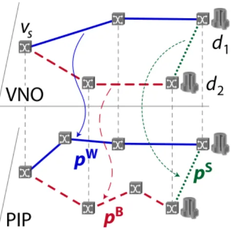
Fig. 1: The VNO-resilience scheme. As illustrated in Fig. 1, the VNO-resilience model provides

1:1 protection routing in the VNet for network failures, where the working and protection paths of a service have to be physically link/node disjoint: the working path (pw_{) routes}

the services towards the primary DC, the protection path (pb₎

towards the backup DC, whilepw_andpb_{are disjoint in their}

physical layer mapping. In addition, a synchronization path (ps_{) is established in order to handle migration and failure}

routing requirements when a DC failure occurs: services then need to be rerouted from the primaryd1to backupd2. Thus,

the resulting VNet for the request from sourcevscomprises

three virtual paths (comprising 5 virtual links in total, in this example), mapped to resp. the physical pw_{, p}b _{and p}s

paths. Note that both pw _{and p}b _{need to carry the overall}

traffic (butpb _{only whenp}w _ord

1 are affected by a failure),

butps_{possibly only a fraction thereof, only to keep the state}

at the backup location d2 synchronized with that of d1 (or

vice versa) to allow smooth migration upon d1 failure (or

Further, we assume that there is an automatic switch-back to the original network path or DC once a fault is repaired, and therefore we allow reusing the same network/DC capacity to protect against other failures: backup capacity is shared. Under the assumptions that (A1) the backup DC has a different location than the primary DC, (A2) pw _{and p}b _{are link disjoint and, (A3)p}w _{and p}s _{are link disjoint,}

protection is guaranteed against any single link failure and any single DC failure. We now qualitatively discuss the various failure cases we protect against:

(i) Failure of link`∈pw_{: the request is rerouted to the backup data centerd}

1, using the backup path

pb_{(which is link disjoint fromp}w_{, thus` /∈p</sub>b<sub>). If`∈p}s_∩pw_{, then as long as the failure is not restored,}

the primary data center d1 cannot be kept in sync with the now operational d2. Thus, right after the

repair of `, the primaryd1 is in stale state, and hence switching back tod1 either suffers from this stale

state or needs to wait some extra time to handle the requests again. The remedy is of course to enforce pw_∩ps _{=∅. (Yet, note that the same issue of a non-synchronized primaryd}

1 clearly also occurs after

the repair ofd1 that failed itself.)

(ii) Failure of link ` ∈ps<sub>\p</sub>w<sub>: there is no immediate issue. Yet, if shortly after `’s repair, working</sub>

path pw _{fails, the switchover to the backup d}

2 (via path pb) suffers from stale state since the failing

ps _{interrupted the synchronization between primary and backup DCs. This can only be remedied by}

providing a second synchronization path pss_{that is link disjoint with p}s_.

(iii)Failure of link`∈pb_{: again no immediate problem arises (since this means thatp}w_{is operational,}

givenpw_∩pb_{=∅). However, if `∈p</sub>s<sub>∩p</sub>b <sub>and shortly after`’s repair the primary path p}w _{(ord1) fails}

– meaning that now_bis followed towards d2 – the secondary data center d2 might not be fully sync’ed

yet. Clearly, this can be remedied by choosing pb_∩ps _{=∅. Yet, the issue is similar to the one of case}

(ii), which obviously remains, even if we takeps_∩pb_=∅.

(iv)Failure of primary DCd1: requests are rerouted to backupd2via thepbpath. Clearly, the failing

d1 cannot be kept in sync with the now operational backupd2. Thus, we might need to wait some time

afterd1’s repair to switch back requests viapw. Any failure that would occur shortly afterd1’s repair and

which would prevent services to remain being served atd2clearly could imply service degradation because

of the unsynchronized d1: (a) failure of ps, (b) failure of pb, or (c) failure of d2. However, protection

against such a failure event requires extra DC resources or extra paths.

2.3. Time-varying Traffic

The motivation of this study is to investigate whether it is worth reconfiguring the primary and the backup paths in order to save bandwidth when the communication traffic pattern changes. Note that this change is not necessarily limited to a scaling of the volume, but also its geographical pattern: when considering large backbone networks (as the ones that we are designing VNets over), they might comprise different time zones where activities are shifted in time, and hence the resulting volume of cloud requests fluctuates differently.

As changing the VNet mapping operations clearly may have an impact on the real-time performance of the cloud requests they are servicing, we propose to investigate three scenarios. In Scenario I (very conservative), we do not allow reconfiguring already established paths. In Scenario II, we only allow reconfiguring backup and/or synchronisation routes (pb _{and/or p}s_{) for traffic that continues from one}

period to the next. In Scenario III, we assume complete freedom and thus also allow to change the primary paths (pw_{). Yet, we always look for the optimal solution (in terms of minimal link bandwidth}

consumed on the PIP layer) with the lowest number of configuration changes.

3. Optimization Model 3.1. Notations

The cloud network is modeled by an undirected graph G= (V, L) where V is the node set (indexed by

v) andLis the link set (indexed by`), for whichω(v) denotes the set of links adjacent tov.

Traffic is defined by the number of service requests (demands), originating from a set of source/service nodes V_S ⊆V, with generic index v_S. To simplify the exposure, we assumeV_S =V from now on. Let K be the set of service requests, indexed by k. K is partitioned: K = Kadd_∪Kleg_{, where K}add _are

Each servicekis characterized by its bandwidth requirement ∆k, its source (or origin)vk, its datacenter

resource requirementRk, andδk (with 0≤δk ≤1), representing the fraction of ∆k that is required for

synchronization between the primary and the backup data center.

LetD ⊆V be the set of data centers (indexed byd), and_capad the resource capacity of data center

d(e.g., in terms of virtual machines). Let nD=|D| be the number of data centers. The current model

assumes (at most) a single data center per node.

3.2. Configurations

The mathematical model we propose relies on the notion of configurations, where a configuration is associated with a set of service requests originating at a given source node. LetC be the overall set of configurations: C = S

v∈Vs

Cv, where Cv is the set of configurations associated with source node v ∈Vs.

We define a configurationc∈Cv by: (i)a set of 3 paths, one primary pathpworiginating atvstowards a

primary data centerdw_{, one backup pathp}b _{originating atvstowards a primary data centerd}b_{, and one}

synchronization paths (ps_{) between the primary and the backup data center, as well as (ii) the service}

requests routed and protected by this set of 3 routes. We protect against single link failures as well as single data center failures.

More formally, in our mathematical model, a configuration is characterized by the given parameters: • pw

`,c(resp.pb`,c) = 1 if link`is used by the working (resp. backup) path of configurationc, 0 otherwise;

• ps

`,c = 1 if link ` is used by the synchronization path ofc between the primary data center and the

backup data center, 0 otherwise; • aw,c

v (resp.abv,c) = 1 if nodev∈VDis selected as the primary (resp. backup) data center, 0 otherwise;

For each link `, let βw

` be the working bandwidth on `, β`b the backup bandwidth on `, and β`s the

bandwidth of Synchronization path on`.

In the context of time-varying traffic, the set of configurations is partitioned as follows: C=Cadd_∪Cleg_,

where Cadd _{is the set of newly generated configurations for the requests ofK}add_.

Cleg_=Cleg bs_∪Cleg w _{is the new set of selected configurations associated withk∈K}leg_{, withC}leg bs

being the configurations for which the working paths is unchanged, andCleg w _{the set of configurations}

in which at least the working path has been modified.

3.3. Objective

We first define the set of variables: • zc

k ∈ {0,1}, c∈ Cadd: decision variable that is equal to 1 if the configuration is selected for a given

servicek, 0 otherwise.

• xleg bs

k ∈ {0,1}, k∈Kleg: decision variable that is equal to 1 if the protection or synchronization paths

or the assigned DC of kis modified (the working path is not modified).

• xleg w

k ∈ {0,1}, k ∈Kleg: decision variable that is equal to 1 if the working path and possibly, the

protection or synchronization paths or the assigned DC ofk, is/are modified.

The objective function should take care of minimizing the overall (working + backup + synchronization) bandwidth requirements, and, in case of ties, and should encourage not to disturb the working paths as a first priority, and, as a second priority, not to disturb the backup/synchronization paths in case the same routing paths can be used for the legacy requests:

min X `∈L (βw ` + βb`+ β`s)· k`k | {z } BW` +_penaldisrupt b X k∈Kleg xleg bs k + penaldisrupt w X k∈Kleg xleg w k (1)

where k`k represents the length of link `, _penaldisrupt b _{and penal}disrupt w _{are weight penalty factors}

such that_penaldisrupt b_≥penaldisrupt w_{, and BW}

`is total bandwidth requirement on a given link`.

Note that in Scenario I, only the first term of (1) is minimized, while the second plays a role only in Scenarios II and III, and the third term only for Scenario III.

3.4. A Generic Model

We next describe a generic model that encompasses all three scenarios. It relies on a decomposition scheme such that the master problem selects the best configurations out of a given set, while the pricing problem generates configurations, see Section 4 for more details. We next describe the master problem.

X c∈Cv z_kc ≥1 k∈Kadd v , v∈V (2) X c∈Cleg bs k z_kc =xleg bs k ; xleg bsk ≤1−z ˜ ck k k∈Kleg (3) X c∈C_vk\(Cleg bs k ∪{ck}) z_kc =xleg w k ; xleg wk ≤1−z ˜ ck k k∈Kleg (4) X v∈V X k∈Kadd v ∪Klegv X c∈Cv ∆kpw`,cz c k =β`w ; X v∈V X k∈Kadd v ∪Kvleg X c∈Cv ∆kδkps`,cz c k =β`s `∈L (5) X v∈V X k∈Kadd v ∪Klegv X c∈Cv ∆kpw`0_,cpb_{`,c</sub>zc<sub>k</sub> ≤β<sub>`}b `0∈L, `∈L\ {`0} (6) X v∈V X k∈Kadd v ∪Klegv X c∈Cv ∆kawv,cpb`,cz c k ≤β`b v∈VD, `∈L (7) X v∈V X k∈Kadd v ∪Klegv X c∈Cv Rk(awv,c+ ab ,c v )z c k ≤capav v∈Vd (8) z_kc ∈ {0,1} c∈C, k∈K; βw `, βb`, βs`∈IR `∈L (9) xleg bs k , xleg wk ∈ {0,1} k∈Kleg. (10)

Constraints (2) take care of granting every new services. Constraints (3) (left equality) detect the legacy services with an identical working path, but a different backup or synchronization path. Constraints (4) (left equality) detect the legacy services with a different working path, and potentially a different backup or synchronization path. Constraints (3) (right equality) and (4) ensure consistency between the values of z˜ck

k and xleg wk , and between the values ofz

˜

ck

k and xleg bsk respectively. Constraints (4) (right

equality) forbid xleg w

k =xleg bsk = 1, i.e., if only the backup (or the synchronization) path is changed,

then we cannot change the primary path without being inconsistent. Constraints (5) and (6) compute the working, synchronization and backup bandwidth requirements, respectively. Constraints (7) take care of the backup bandwidth requirement in order to be protected against a single data center failure. Constraints (7) guarantee sufficient backup bandwidth ` to handle any data center failure. Constraints (8) check that the capacity (_capav) of the data centers (v ∈Vd) is not exceeded. The last three set of

constraints, i.e., (9) and (10), define the domain of the variables.

4. Solution Scheme

RMP   Selec)on  of  the  best  

configura)ons  

Solve  PPADD  (k)/PPLEG  (k)  

Genera)on  of  a  new   promising  configura)on   Yes No: select another request (k) All  k  requests   Unsuccessfully   tested   LP  is   op)mally   solved   Find  an    ε–op)mal  

ILP  solu)on   Yes No

RMP Output / PP Input:

No

PP Output / RMP Input:

A new promising configuration ck for request k Values of the dual variables

(check ck for all the other configurations In order to avoid duplicating configurations)

Nega)ve   reduced  cost?  

Fig. 2: Solution Process The above master problem (RMP) is solved

itera-tively, alternating with the solution of the pricing problem (PP) that determines augmenting config-urations, i.e., routes for _w, _b and _s paths such that their addition to the restricted master prob-lem entails an improvement of the optimal value of the current restricted master problem, see the flowchart in Fig. 2. Each PP is written for a given source nodevk and for a given request originating

atvk. Parameters ∆kandδkretain their definition

for a request kas in the RMP.

The sets of variables corresponds to the set of parameters in the master problem, i.e.,pw

`,pb`,ps`,

aw

v, abv, dwv, dbv and dsv. We need to distinguish

two pricing problems, one for the requests newly added in the considered period (_add), another one

While the pricing problem is solved for a given request, say k, we check whether it allows to generate augmenting configurations for all the requests with the same origin node as k. In other words, if an augmenting configuration is found fork, we check whether it is also an augmenting configuration for any k0 from the same source, i.e., for whichvk0 =v_k. If it is the case, we addc_k to the set of configurations

associated withk0. Once we have examined allk0 such thatvk0=v_k, the next PP is solved for a request

with a different source node. This way, instead of a number of iterations in the order of the number of requests — which can be quite computationally expensive — we expect a complete round to be in the order of the number of source nodes.

For a given source node, requests are initially ordered according to decreasing bandwidth requirements, but we examine in a round robin fashion from one round to the next, in order not to always start solving the pricing problem for the same request.

The objective of PP_add(k) withk∈Kadd_{is to minimize the reduced costcost}add_(z

k), which is

straight-forwardly derived from the RMP — see [9] if not familiar with linear programming tools. Note that two quadratic terms appear in the reduced cost (i.e., those associated with the dual variables of (6) and (7)), but they can be easily linearized through the introduction of two sets of binary variables pwb

``0 and pwb_v`

and the addition of the following constraints, for all`0∈L, `∈L\ {`0_{}, v∈V}

d:

pwb

``0 ≤pw<sub>`</sub>0 ; pwb<sub>``</sub>0 ≤pb_{`</sub> ; pwb<sub>``</sub>0 ≥pw<sub>`}0+pw_{`</sub>0−1 ; pwb<sub>v`} ≤aw_v ; pwb_{v`</sub> ≤p<sub>`}b ; pwb_{v`</sub> ≥aw<sub>v</sub> +pw<sub>`}0−1.

To complete the PP, we need to enforce that the path and data center variables obey the following constraints1_{: the flow constraints for the undirected working, backup and synchronization paths, the link}

disjointness constraints of pathsp_wandp_b, and the fact that each configuration has exactly one primary and one back up data center, while primary and backup data centers are different.

Now, for the legacy constraints, we have a slightly different PP_leg. In short, the only change is that for these requests, the path changes that we can make are restricted, depending on the scenario (recall Section 2.3). In Scenario I, the full routing of these requests is given from the first period, so we do not need to solve any PP for them. In Scenario II, we cannot change the working path and thus the corresponding values ˜pW

` are given a priori, while the other paths follow similar constraints as in PPadd.

For Scenario III, we have the full flexibility and thus the PP is the same as in the_addcase. In all cases, fork∈Kleg_{, the expression ofcost}leg_(z

k) is easily derived fromcostadd(zk).

5. Numerical Results 5.1. Data Sets

We used the USA network illustrated in Fig. 3, which we divided into three regions, each with their own traffic pattern. Each request is randomly generated with a bandwidth requirement (∆k) normalized

between 0 and 1, and aδk = 0.1 synchronization factor. We assume 4 data centers, located in CA (node

5), WY(node 6), TX (node 13), OH (node 15). We consider the transition from one period to a next, where the eventual number of requests varies from 20 to 80 requests. While this total remains the same among the two successive periods, the geographical distribution of their origins changes from the first to the second period. Initially, i.e., during the first planning time period, the traffic is distributed as follows: 30% in region 1, 50% in region 2, and 20% in region 3. For each of those regions, sources are uniformly randomly spread over the nodes within the respective region. Next, during the second time period, the traffic is randomly modified (again uniformly distributed over nodes within each region): the traffic of period 1 that continues into period 2, designated aslegacy traffic, varies per region as indicated in Table 1. We consider three scenarios, where the overal legacy traffic (over all three regions together) is set to 40%, 60%, and 80% respectively.

5.2. Bandwidth Requirements with Time-varying Traffic

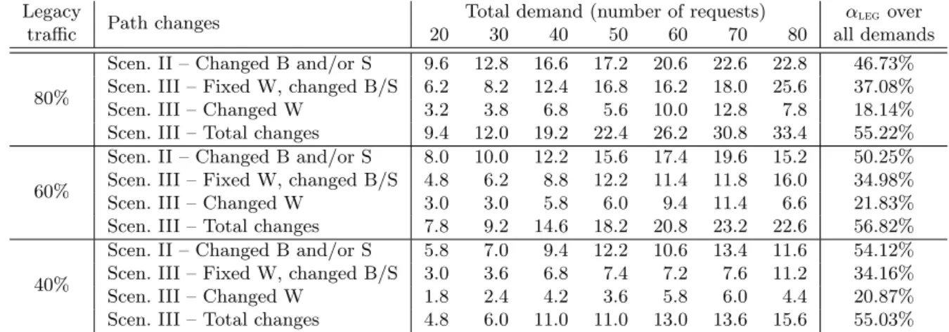
We conducted experiments under different traffic loads and computed the bandwidth requirements under different backup provisioning scenarios as described in Section 2.3. For each traffic load, results correspond to averages over 5 data instances. The observations from the results plotted in Fig. 4 are as follows:

1_{Since these constraints are straightforward to write down for anyone familiar with linear programming, we omit the}

1 2 6 3 4 7 5 8 10 14 13 17 18 24 23 22 16 11 15 21 20 19 9 ₁₂ 1000 1000 1000 1000 1000 1000 1000 1000 1000 1000 1100 1100 1150 1200 1200 1200 1200 1300 1300 1400 1900 2600 900 900 900 950 950 800 850 850 1000 800 800 800 800 850 900 250 600 300 700 600 650

Region 1 Region 2 Region 3

Fig. 3: USA network with its different regions.

Table 1: Traffic change distribution over the three regions, where the change is expressed in % of the total traffic volume summed over all regions.

Scenario Region 1 Region 2 Region 3

40% 20%_drop 30%_drop 10% _drop

legacy 20%_add 10%_add 30% _add

60% 10%_drop 20%_drop 10% _drop

legacy 10%_add 10%_add 20% _add

80% 10%_drop 10%_drop –

legacy 10%_add – 10% _add

80% legacy traffic 60% legacy traffic 40% legacy traffic

●●● ●●● ●●● ●●● ●●● ●● ● ●●_● ●●● ●●● ●●● ●●● ●●● ●● ● ●●● ●●● ●●● ● ●● ●●● ●●● ●●● ●●● 0e+00 5e+04 1e+05 30 50 70 30 50 70 30 50 70 Number of requests Bandwidth (summed o v er all links) ● Total Working (W) Backup (B) Synchronisation (S) Scenario I

(no changes for legacy) Scenario II

(change only B and/or S) Scenario III

(change B, S, and/or W)

Fig. 4: Bandwidth requirements.

• Bandwidth savings are not significant as long as we do not allow disruption, i.e., reconfiguration, of some working paths (from Scenario I to II the cost difference is not big, but for Scenario III it is). • Bandwidth savings mainly stem from the reduction of backup capacity (for all three legacy traffic

cases).

• The bandwidth for the synchronization among primary and backup data centers (the ps_{), even if}

provisioned on different paths, is rather constant for all three reconfiguration scenarios.

• The achieved bandwidth savings (for Scenario III), relative to the total cost, decreases with decreasing the fraction of legacy traffic (obviously, since the savings come from changing legacy requests, if there are fewer of them then the saving potential diminishes).

Now, one may wonder what the amount of path reconfigurations is that is required to achieve those band-width savings (esp. for Scenario III). This we have summarized in Table 2. This shows that in Scenario III, even though more than half of the legacy requests need to have some of their paths reconfigured, only around 20% of them require a change of the working path. Thus, if we may assume that a sufficient fraction of the traffic does not have QoS requirements that prohibit path reconfiguration, this may be an acceptable solution to cut down the VNet operating costs in terms of needed PIP resources.

6. Conclusion

We investigated the interest of re-provisioning the working and the backup paths in the context of anycast routing traffic in cloud computing, assuming time-varying traffic, where the path provisioning can be updated periodically. While it seems that periodic backup reconfiguration is only advantageous if we reconfigure some working paths as well, further experiments should evaluate the impact of the server locations (e.g., scattered vs. paired as in [10]), and investigate different time-varying traffic patterns.

Table 2: Number of requests that need reconfigurations (W = of the working path, B = of the backup path, S = of the synchronisation path). The last column shows the fraction of modified legacy requests (α_leg), averaged over all demand instances.

Legacy

Path changes Total demand (number of requests) αlegover

traffic 20 30 40 50 60 70 80 all demands

80%

Scen. II – Changed B and/or S 9.6 12.8 16.6 17.2 20.6 22.6 22.8 46.73% Scen. III – Fixed W, changed B/S 6.2 8.2 12.4 16.8 16.2 18.0 25.6 37.08% Scen. III – Changed W 3.2 3.8 6.8 5.6 10.0 12.8 7.8 18.14% Scen. III – Total changes 9.4 12.0 19.2 22.4 26.2 30.8 33.4 55.22%

60%

Scen. II – Changed B and/or S 8.0 10.0 12.2 15.6 17.4 19.6 15.2 50.25% Scen. III – Fixed W, changed B/S 4.8 6.2 8.8 12.2 11.4 11.8 16.0 34.98% Scen. III – Changed W 3.0 3.0 5.8 6.0 9.4 11.4 6.6 21.83% Scen. III – Total changes 7.8 9.2 14.6 18.2 20.8 23.2 22.6 56.82%

40%

Scen. II – Changed B and/or S 5.8 7.0 9.4 12.2 10.6 13.4 11.6 54.12% Scen. III – Fixed W, changed B/S 3.0 3.6 6.8 7.4 7.2 7.6 11.2 34.16% Scen. III – Changed W 1.8 2.4 4.2 3.6 5.8 6.0 4.4 20.87% Scen. III – Total changes 4.8 6.0 11.0 11.0 13.0 13.6 15.6 55.03%

ACKNOWLEDGMENT

B. Jaumard has been supported by a Concordia University Research Chair (Tier I) and by an NSERC (Natural Sciences and Engineering Research Council of Canada) grant. D. Medhi has been supported by National Science Foundation Grant No. CNS-1217736.

REFERENCES

[1] X. He and G.-S. Poo, “Sub-reconfiguration of backup paths based on shared path protection for WDM networks with dynamic traffic pattern,” in Proc. 9th Int. Conf. Commun. Systems (ICCS), Sep. 2004, pp. 391–395.

[2] S. Srivastava, S. R. Thirumalasetty, and D. Medhi, “Network traffic engineering with varied levels of protection in the next generation internet,” in Performance Evaluations and Planning Methods for the Next Generation Internet, A. Girard, B. Sanso, and F. Vazquez-Abad, Eds. Springer Verlag, 2005.

[3] S. Sebbah and B. Jaumard, “Differentiated quality-of-protection in survivable wdm mesh networks usingp-structures,”Computer Commun., vol. 36, pp. 621–629, Mar. 2013.

[4] C. Develder, J. Buysse, B. Dhoedt, and B. Jaumard, “Joint dimensioning of server and network infrastructure for resilient optical grids/clouds,”IEEE/ACM Trans. Netw., pp. 1–16, Oct. 2013. [5] M. Bui, B. Jaumard, and C. Develder, “Anycast end-to-end resilience for cloud services over virtual

optical networks (invited),” inProc. 15th Int. Conf. Transparent Optical Netw. (ICTON), Cartagena, Spain, 23–27 Jun. 2013.

[6] C. Develder, M. De Leenheer, B. Dhoedt, M. Pickavet, D. Colle, F. De Turck, and P. Demeester, “Optical networks for grid and cloud computing applications,” Proc. IEEE, vol. 100, no. 5, pp. 1149–1167, May 2012.

[7] N. Chowdhury and R. Boutaba, “A survey of network virtualization,”Computer Netw., vol. 54, pp. 862–876, Apr. 2010.

[8] P. Primet Vicat-Blanc, S. Soudan, and D. Verchere, “Virtualizing and scheduling optical network infrastructure for emerging IT services,”J. Optical Commun. Netw., vol. 1, pp. A121–A132, 2009. [9] V. Chvatal,Linear Programming. Freeman, 1983.

[10] M. Bui, B. Jaumard, and C. Develder, “Resilience options for provisioning anycast cloud services with virtual optical networks,” in Proc. IEEE Int. Conf. on Commun. (ICC), Sydney, Australia, 10–14 Jun. 2014.