Centre for Central Banking Studies

(1)

Centre for Central Banking Studies

Joint Research Paper – No. 3

Money-based inflation risk indicator for Russia:

a structural dynamic factor model approach

(2)

Money-based inflation risk indicator for Russia: A structural dynamic

factor model approach

1

Elena Deryugina2

Alexey Ponomarenko3

Abstract

We estimate a dynamic factor model for the cross-section of monetary and price indicators. We extract the common part of the dataset’s fluctuations and decompose it into structural shocks. We argue that one of the shocks identified has empirical properties (in terms of impulse response functions) that are fully in line with the theoretically expected relationship between money growth and inflation, confirming that the process identified has the capacity for economic interpretation. Based on this finding, we decompose recent inflationary developments in Russia into those that are associated with changes in monetary stance and other shorter-lived shocks. We show that the underlying monetary component of future inflation may be projected accurately based on the observed monetary developments.

Keywords: Monetary aggregates, inflation, dynamic factor model, transition countries

JEL classification: C22, E31, E51.

1_{The views expressed in this paper are those of the authors. They do not necessarily represent the position of the}

Bank of Russia. We are grateful to the participants of the joint ECB/Bank of Russia Seminar on Monetary Analysis and would like to thank Haroon Mumtaz from CCBS, Bank of England for his assistance. Charlotte Dendy provided excellent research assistance and Maria Brady provided valuable administrative support.

2_{Research and Information Department, Bank of Russia. E-mail:}_{[email protected]} 3_{Research and Information Department, Bank of Russia. E-mail:}_{[email protected]}

(3)

1.

Introduction

The analysis of the monetary determinants of inflation is of obvious interest for countries that pursue a price stability objective. As discussed in Papademos and Stark (2010), monetary aggregates are apparently useful in the identification of inflation risks in particular in the long run. For Russia (as well as presumably for many other transition countries) the necessity of relying on monetary indicators to monitor inflation risks seems especially evident for a number of reasons. First, money stock may arguably be regarded as the most comprehensive monetary stance indicator for the Russian economy. This is to a large degree, due to the fact that monetary and fiscal policy measures, (such as the Bank of Russia’s forex purchases or sovereign funds management) may have a direct effect on money supply without being reflected in the levels of policy interest rates (see Ponomarenko et al. 2012 for a review).4 On the other hand, for transition economies, it may also be challenging to identify demand-side inflationary pressures based on real sector indicators, e.g. the output gap, while growth rates fluctuate dramatically as the economy undergoes substantial transformation.

Admittedly, monetary analysis of inflation is far from being immune from such problems. For example, models of inflation that are required to identify a stable money demand relationship (as in the VECM framework; see e.g. Korhonen and Mehrotra 2010) or in order to estimate excess liquidity measures (see e.g. Oomes and Ohnsorge 2005) may fail to do so in a rapidly developing financial environment. Furthermore, a significant part of the consumer price index (CPI) measure in Russia is composed of food and administered prices predetermining the indicator’s high volatility. Therefore attempts to link all CPI fluctuations with, especially monetary, fundamentals may potentially be misleading. In theory, one may try to overcome this problem by smoothing the inflation rate over longer horizons (e.g. as outlined in Chapter 4 of Papademos and Stark 2010, and employed in Ponomarenko et al. 2012), although this approach might also require a longer time sample than is currently available for Russia.

Against this background, we evaluate the information content of money with regard to inflation developments in the spirit of Nobili (2009), i.e. by applying the dynamic factor model approach on a cross-section of variables comprising the broad monetary aggregates, as well as their components and the collection of different price indices. Our statistical approach aims at

4_{In fact considering the relative insignificance of interbank money markets (particularly domestic) in Russia and the}

high volatility of short-term interest rates, it is doubtful that any money market interest rate or any of the Bank of Russia’s interest rates per se could safely be regarded as a policy rate over the last decade.

(4)

extracting the underlying monetary process that is most relevant for inflation by weighting the monetary aggregates according to their signal to noise ratio, namely, down-weighting those with large idiosyncratic variances. Presumably, our approach should downplay those monetary instruments, the developments of which are affected by financial innovation as well as portfolio considerations. In addition, it should also weight money holdings at the sectoral level as money held by different sectors may have different properties for inflation. Simultaneously, given that we rely on a range of price indicators to reflect inflation developments, we expect to filter out the volatile component of CPI that might otherwise distort the relationship with money growth.

The paper is structured as follows. Section 2 provides the general description of the dataset used for the estimation. Section 3 presents the formal model. Section 4 presents the empirical results and discusses possible applications of the model. Section 5 concludes.

2.

Data

There are many macroeconomic variables that may potentially be part of a monetary driven price growth process. Clearly some part of monetary developments, for example induced by portfolio shifts or other money demand shocks, may have no inflationary consequences just as prices may be subject to non-monetary shocks. However, if these shocks are variable specific, we may be able to identify the monetary inflation process by extracting the common part of the reviewed variables. With this purpose we compiled our dataset from variables in two general categories.

The first category is monetary aggregates. Money supply in Russia is usually measured in terms of national money stock (M2) or broad money (M2X). We included these two measures in our dataset, along with their components. The broad monetary aggregates were decomposed along three dimensions:

 by liquidity of monetary instruments: we separated M1 (cash and demand deposits) and time deposits;

 by institutional sector: we separated households (HH) and non-financial corporations (NFC);5

 by currency of denomination (ruble or foreign currency).6

We also added the Divisia aggregate of M2 and the estimate of foreign cash in circulation.7

5_{The money holdings of other financial institutions in Russia are insignificant. We therefore see no reason to}

include these as a separate component.

6_{As in Ponomarenko et al. (2012), the foreign currency denominated aggregates were adjusted for a re-evaluation}

(5)

The second category of our dataset is price indices. The conventional price indicator in Russia is CPI (e.g. the Bank of Russia’s inflation target is formulated in terms of this index). We included the headline CPI measure along with three sub-indices: core, food and non-food inflation. We also added the deflator of three SNA indicators: fixed capital investment, domestic absorption and GDP. Finally we added housing price indices (for primary and secondary markets).

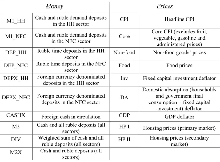
This gave us a dataset consisting of 10 monetary and nine price indicators.

Table 1. Dataset

Money Prices

M1_HH Cash and ruble demand deposits

in the HH sector CPI Headline CPI

M1_NFC Cash and ruble demand deposits

in the NFC sector Core

Core CPI (excludes fruit, vegetable, gasoline and

administered prices) DEP_HH Ruble time deposits in the HH

sector Non-food Non-food goods’ prices DEP_NFC Ruble time deposits in the NFC

sector Food Food prices

DEPX_HH Foreign currency denominated

deposits in the HH sector Inv Fixed capital investment deflator

DEPX_NFC Foreign currency denominated

deposits in the NFC sector DA

Domestic absorption (households and government final consumption + fixed capital

investment) deflator CASHX _{Foreign cash in circulation} GDP _{GDP deflator}

M2 Cash and all ruble deposits (all

sectors) HP I Housing prices (primary market) DIV Weighted sum of cash and all

ruble deposits (all sectors) HP II

Housing prices (secondary market)

M2X Cash and ruble deposits (all sectors)

These data were obtained from Rosstat and Bank of Russia databases. The series are quarterly frequencies in the form of annual growth rates and standardized. The time sample is from 2003 Q4 to 2012 Q3. The series are presented in the Annex along with the results of unit root tests that confirm stationarity.

7_{Although this indicator is not part of conventional monetary aggregates and could presumably be subject to}

significant measurement error, it may regarded as an important monetary instrument in the Russian economy (at least in the early 2000s). The estimate was constructed as in Ponomarenko et al. (2012).

(6)

3.

Methodology

3.1 The theoretical factor model

Our empirical strategy is based on the generalized dynamic factor model proposed by Forni et al. (2000) and Forni and Lippi (2001). Consider a set of variables where each variable xit is the sum of two mutually orthogonal unobservable components, the common component

χ

it and the

idiosyncratic component

ξ

it:

xit =

χ

it +

ξ

it. (1)

The idiosyncratic components are not correlated in the cross-sectional dimension. They arise from shocks or sources of variation which considerably affect only a single variable; in this sense, they are not underlying shocks. In our case these could be portfolio shifts between monetary instruments or price shocks affecting particular types of goods or services that are not part of the prevailing inflation trend.

The common components are responsible for the main bulk of the co-movements between the variables, being linear combinations r of factors f1t ; f2t ; . . . ; frt , not depending on i:

χ

it = a1i f1t + a2i f2t +…+ ari frt = aift. (2)

The dynamic relations between the macroeconomic variables arise from the fact that the vector ft

of the common factors follows the VAR relation:

ft = D1 ft-1 + … + Dp ft-p +

ε

t, (3)

ε

t =Rut, (4)

where R is a r × q matrix and ut = (u1t u2t … uqt) is a q-dimensional vector of orthonormal white

noises, with q ≤r. Such white noises are “dynamic factors” (whereas the entries of ft are “static

factors”). The variables themselves can be expressed as:

xit = bi(L)ut+

ξ

it, (5)

(7)

bi(L) = ai(I-D1L- … - DpLp)-1R. (6)

The dynamic factors ut and bi(L) are assumed to be structural macroeconomic shocks and

impulse response functions, respectively.

3.2 The state space representation of the factor model

In order to estimate our model, we formulated it in the state space form which is one of the conventional approaches (see e.g. Stock and Watson 2011 for a review):

it t i it

a

F

v

X





(7)



 





L j t j t j t

D

F

e

F

1



(8)

e

t = R

ut

(9)

The “observation” part of the model (7) consists of the set of equations where the monetary and price variables (Xit) are explained by static factors (Ft). The fitted part (aiFt) is considered to be

the common component while the unexplained part (vit) is considered to be the idiosyncratic

component of the respective variable. The “transition” part of the model (8) consists of the VAR model comprising the static factors. The structural shocks (

ut

) are subsequently extracted from the VAR’s residuals (

e

t). Similarly to standard SVAR models, the impulse response functions

and historical decompositions of deviations from baseline projections associated with these shocks, may be estimated for static factors and more importantly, for the common component of every macroeconomic variable in the model.

We estimated our model using Bayesian methods as described in Blake and Mumtaz (2012). We used principal components analysis to obtain initial estimates of static factors Ft. A detailed

description of the prior distributions and the sampling method is given in Chapter 3.7 of Blake and Mumtaz (2012). We made 60,000 iterations, increasing this number further does not change the results, presumably indicating the attainment of convergence and accepted the last 5,000 models. The median output of these models is presented as the result, for example the impulse response functions and historical decompositions. The application of Bayesian methods seems appropriate as it yielded robust and stable results, compared to canonical econometric methods,

(8)

on the relatively short Russian time sample. The number of static factors (Ft) was set to three.8

Accordingly, we may identify up to three structural shocks. The lag length of the VAR was set to

L=2.9

3.3 Identification of structural shocks

Structural interpretations of dynamic factor models are not conducted ordinarily (e.g. Nobili 2009 only identifies common and idiosyncratic processes), although it is clearly not unprecedented (see Forni et al. 2009, Forni and Gambetti 2010). We believe that valuable insight may be gained by examining the macroeconomic properties of the identified common shocks in more detail.

To this effect we extracted principal components from residuals series

e

t, decomposing them into

three mutually independent processes

ut

(this approach is described in Forni et al. 2009). Accordingly, matrix R comprises the respective loading coefficients. We will examine the macroeconomic relevance of these shocks in Section 4.

Admittedly, the adopted identification scheme is not unique and just as in the case of standard VAR models, other ways of extracting structural shocks may be proposed. Naturally, one of these is recursive estimation using the Cholesky decomposition. We have checked that application of this approach does not significantly change the properties of the identified shocks compared to a principal components approach. Another possible method would be to impose theoretically motivated restrictions on impulse response functions and search for conforming structural shocks (Uhlig 2005). This approach seems appropriate here but, as discussed in Section 4.1, at least one of the structural shocks identified via the principal components method is associated with impulse response functions that match the theoretical expectations for the money growth–inflation relationship. We therefore see no reason to impose such restrictions a priori. On these grounds we conclude that our results are robust in terms of the choice of an identification scheme for structural shocks.

8_{As pointed out in Forni and Gambetti (2010), a large number of static factors are needed to allow for}

cross-sectional dynamic heterogeneity among variables (i.e. leading or lagging relationship). We obviously expect to find such a relationship between money and prices and therefore are willing to include many static factors in the model. However, we found that adding more than three static factors leads to non-stationarity of the VAR. As discussed in Section 4.2, this number of static factors allows us to obtain a reasonable share of explained cross-sectional variance.

9_{The model seems to be robust in relation to the lag length choice: setting}_L_{=3 or}_L_{=4 does not change the results}

(9)

4.

Results

4.1

Impulse response analysis

In this section we examine the empirical properties of identified structural shocks by observing their impact on macroeconomic variables in our dataset.

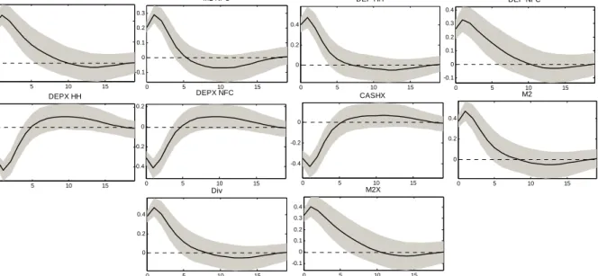
The impulse response functions that are associated with the first shock seem to be crucial for our research since they exhibit a distinct and economically meaningful pattern. The shock causes a contemporaneous increase in the growth of broad monetary aggregates (M2 and M2X) that subsequently dies out over the next five quarters. This is followed by prolonged acceleration of all price growth indices that in most cases peaks in six to eight quarters (four quarters in the case of housing prices) and ceases in 10–12 quarters. Such a relationship seems to be fully consistent with theoretical beliefs regarding the profile of monetary induced inflation occurrence, as well as with empirical evidence regarding the lag-lead structure (see e.g. Nicoletti-Altimari 2001). The fact that asset price inflation in Russia may be closely linked to monetary developments has also been reported previously (e.g. Mehrotra and Ponomarenko 2010, Mumtaz et al. 2012).

More detailed analysis of impulse response functions also reveals several features distinctive for the Russian economy. As discussed in Ponomarenko et al. (2012), prior to 2009, money supply fluctuations in Russia were closely related to flows of oil and gas export revenues. An increase in oil and gas revenue, e.g. due to a commodity price shock, would also cause ruble appreciation (or at least generate appreciation expectations). This in turn would trigger portfolio shifts in the denomination of assets from foreign currency to the ruble (see Ponomarenko et al. 2013 for a review of (de)dollarization in Russia). Presumably this kind of reaction is reflected in the negative response functions of foreign currency components to the overall positive money supply shocks obtained. Exchange rate appreciation could also account for the initial short-lived negative response observed for some price indices.10 The fact that average money supply shock in Russia was associated with commodity price shocks is also presumably reflected in the contemporaneous response of the GDP deflator that includes export prices.

Overall, we conclude that the impulse response functions obtained provide adequate characterization of a typical money supply shock in Russia. On these grounds we consider the

10_{The fact that this effect predominantly shows up in non-food inflation seems plausible as this category of goods is}

(10)

first identified shock to be structural in the macroeconomic sense and label it the “monetary” shock.

Figure 1a. Impulse responses of money to Shock I (the “monetary” shock) (confidence band is set by 16% and 84% quantiles)

0 5 10 15 0 0.2 0.4 M1 HH 0 5 10 15 -0.1 0 0.1 0.2 0.3 M1 NFC 0 5 10 15 0 0.2 0.4 DEP HH 0 5 10 15 -0.1 0 0.1 0.2 0.3 0.4 DEP NFC 0 5 10 15 -0.4 -0.2 0 0.2 DEPX HH 0 5 10 15 -0.4 -0.2 0 0.2 DEPX NFC 0 5 10 15 -0.4 -0.2 0 CASHX 0 5 10 15 0 0.2 0.4 M2 0 5 10 15 0 0.2 0.4 Div 0 5 10 15 -0.1 0 0.1 0.2 0.3 0.4 M2X

Figure 1b. Impulse responses of prices to Shock I (the “monetary” shock) (confidence band is set by 16% and 84% quantiles)

0 2 4 6 8 10 12 14 16 18 -0.2 -0.1 0 0.1 0.2 0.3 CPI 0 2 4 6 8 10 12 14 16 18 -0.2 0 0.2 Core 0 2 4 6 8 10 12 14 16 18 -0.3 -0.2 -0.1 0 0.1 0.2 Non-food 0 2 4 6 8 10 12 14 16 18 -0.1 0 0.1 0.2 0.3 0.4 HP I 0 2 4 6 8 10 12 14 16 18 -0.1 0 0.1 0.2 0.3 0.4 HP II 0 2 4 6 8 10 12 14 16 18 -0.1 0 0.1 0.2 0.3 DA 0 2 4 6 8 10 12 14 16 18 -0.1 0 0.1 0.2 0.3 Inv 0 2 4 6 8 10 12 14 16 18 0 0.1 0.2 0.3 GDP 0 2 4 6 8 10 12 14 16 18 -0.2 -0.1 0 0.1 0.2 0.3 Food

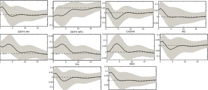
The impulse response functions of the second identified shock indicates its irrelevance to monetary aggregates. This shock only produces a significant contemporaneous impact on price indices, although not on housing prices. Under this set up, we may say nothing regarding the economic nature of these price shocks, except that they are not related to monetary factors.

(11)

Figure 2a. Impulse responses of money to Shock II (confidence band is set by 16% and 84% quantiles) 0 5 10 15 -0.1 -0.05 0 0.05 0.1 M1 HH 0 5 10 15 -0.1 -0.05 0 M1 NFC 0 5 10 15 -0.1 -0.05 0 0.05 0.1 DEP HH 0 5 10 15 -0.05 0 0.05 0.1 DEP NFC 0 5 10 15 -0.05 0 0.05 0.1 0.15 DEPX HH 0 5 10 15 -0.05 0 0.05 0.1 0.15 DEPX NFC 0 5 10 15 -0.05 0 0.05 0.1 0.15 CASHX 0 5 10 15 -0.1 -0.05 0 0.05 0.1 M2 0 5 10 15 -0.1 -0.05 0 0.05 0.1 Div 0 5 10 15 -0.05 0 0.05 0.1 0.15 M2X

Figure 2b. Impulse responses of prices to Shock II (confidence band is set by 16% and 84% quantiles) 0 2 4 6 8 10 12 14 16 18 -0.05 0 0.05 0.1 0.15 0.2 CPI 0 2 4 6 8 10 12 14 16 18 0 0.1 0.2 Core 0 2 4 6 8 10 12 14 16 18 -0.05 0 0.05 0.1 0.15 Non-food 0 2 4 6 8 10 12 14 16 18 -0.05 0 0.05 0.1 0.15 HP I 0 2 4 6 8 10 12 14 16 18 -0.05 0 0.05 0.1 0.15 HP II 0 2 4 6 8 10 12 14 16 18 0 0.1 0.2 Inv 0 2 4 6 8 10 12 14 16 18 -0.05 0 0.05 0.1 0.15 0.2 DA 0 2 4 6 8 10 12 14 16 18 -0.05 0 0.05 0.1 0.15 GDP 0 2 4 6 8 10 12 14 16 18 -0.05 0 0.05 0.1 0.15 0.2 Food

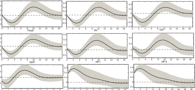
The third identified shock causes the gradual acceleration of broad and most of the narrower ruble monetary aggregates and indistinct cyclical fluctuations of most of price indices. One may speculate that this shock represents a money demand shock based on the general considerations that money demand shocks are those monetary developments that affect money stock without affecting inflation. This hypothesis may be supported by the fact that the acceleration of monetary aggregates is preceded by a distinct increase in housing prices that could be regarded as one of the money demand determinants (Mehrotra and Ponomarenko 2010, Ponomarenko et al. 2012). However, admittedly our model is not particularly suitable for the analysis of money demand or asset price developments. We will therefore abstain from economic interpretation of this shock.

(12)

Figure 3a. Impulse responses of money to Shock III (confidence band is set by 16% and 84% quantiles) 0 5 10 15 -0.1 0 0.1 0.2 0.3 M1 HH 0 5 10 15 -0.1 0 0.1 0.2 M1 NFC 0 5 10 15 -0.1 0 0.1 0.2 0.3 DEP HH 0 5 10 15 -0.1 0 0.1 0.2 DEP NFC 0 5 10 15 -0.3 -0.2 -0.1 0 0.1 0.2 DEPX HH 0 5 10 15 -0.2 -0.1 0 0.1 0.2 DEPX NFC 0 5 10 15 -0.2 -0.1 0 0.1 0.2 CASHX 0 5 10 15 -0.1 0 0.1 0.2 0.3 M2 0 5 10 15 -0.1 0 0.1 0.2 0.3 Div 0 5 10 15 -0.1 0 0.1 0.2 0.3 M2X

Figure 3b. Impulse responses of prices to Shock III (confidence band is set by 16% and 84% quantiles) 0 2 4 6 8 10 12 14 16 18 -0.2 -0.1 0 0.1 0.2 0.3 CPI 0 2 4 6 8 10 12 14 16 18 -0.2 -0.1 0 0.1 0.2 0.3 Core 0 2 4 6 8 10 12 14 16 18 -0.3 -0.2 -0.1 0 0.1 0.2 Non-food 0 2 4 6 8 10 12 14 16 18 -0.1 0 0.1 0.2 0.3 HP I 0 2 4 6 8 10 12 14 16 18 -0.1 0 0.1 0.2 0.3 HP II 0 2 4 6 8 10 12 14 16 18 -0.1 0 0.1 0.2 0.3 Inv 0 2 4 6 8 10 12 14 16 18 -0.1 0 0.1 0.2 DA 0 2 4 6 8 10 12 14 16 18 -0.1 0 0.1 0.2 GDP 0 2 4 6 8 10 12 14 16 18 -0.2 -0.1 0 0.1 0.2 0.3 Food

Hence we conclude that of the three identified shocks one has evident properties of a money– inflation relationship and therefore may have a structural macroeconomic interpretation. Therefore, it may be useful to further decompose the estimated common component of the variables and extract the fluctuations associated with this “monetary” shock separately.

(13)

4.2

Commonality analysis

In this section we compare the variance of the estimated common component with the total variance of the variables. On the one hand, this ratio may be regarded as an indicator of the model’s explanatory power. On the other hand, it may be considered a commonality criterion and accordingly provides an insight into the relevance of different variables for the money– inflation relationship. Similarly to standard SVAR models, the common component may be further decomposed into the baseline projection and fluctuations caused by structural shocks (we will review one of such decompositions in more detail in the next section). We review separately the variance of the whole common component and the variance of the fluctuations associated with the “monetary” shocks identified earlier.

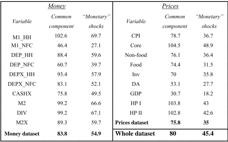
The overall share of the dataset’s explained variance (80%) seems to be adequate and comparable with the results obtained previously (e.g. Nobili 2009). The model seems to explain the monetary and price indicators with equal measure. The variable specific results are more heterogeneous but seem to be generally acceptable. There are only two variables (M1 in the NFC sector and the GDP deflator) where less than half of the variance is explained. Given that there are also cases when the common component’s variance is actually greater than variable’s own variance, trying to improve the model’s fit further seems unfeasible.

More than half of the explained variance comes from the “monetary” shocks, which we find reassuring. Monetary aggregates generally seem to be more liable to these shocks than prices (55% and 35% of explained variance, respectively). One could conclude that although most monetary developments are relevant for prices only, a little more than one third of variance in actual inflation is associated with monetary factors. The variable specific results seem to be in line with expectations. The least noisy, in terms of the informational content relevant to inflation, are broad monetary aggregates and the M1 aggregate in the household sector. Among price indices, the core inflation measure seems to have the closest link with monetary developments as well as, interestingly, housing prices.

(14)

Table 2. Variance of the common component as a percentage of a variable’s total variance (%)

Money Prices

Variable Common component “Monetary” shocks Variable Common component “Monetary” shocks M1_HH 102.6 69.7 CPI 78.7 36.7 M1_NFC 46.4 27.1 Core 104.5 48.9 DEP_HH 88.4 59.6 Non-food 76.1 36.4 DEP_NFC 60.7 39.7 Food 74.4 31.5 DEPX_HH 93.4 57.9 Inv 70 35.8 DEPX_NFC 83.1 52.1 DA 53.1 27.7 CASHX 75.8 49.5 GDP 30.7 18.2 M2 99.2 66.6 HP I 103.8 43 DIV 99.2 67.1 HP II 102.8 42.6 M2X 89.3 59.7 Prices dataset 75.8 35

Money dataset 83.8 54.9

Whole dataset

80

45.4

4.3

Historical decomposition of inflation

In this section we present the decomposition of CPI inflation into fluctuations determined by identified common shocks (including “monetary” shocks) and the unexplained idiosyncratic component. We find this type of analysis exceptionally informative and useful for assessment of inflationary risks. Arguably, the inflationary developments that are associated with fundamental factors deserve full attention from the policy maker while others should be treated more cautiously. This is because the latter are not usually related to monetary policy stance, but also they are likely to be short-lived.

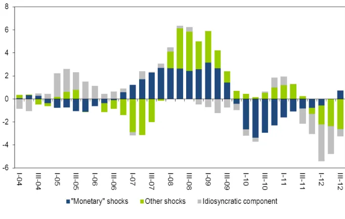
The results obtained seem economically meaningful and may be interpreted consistently. The impact of “monetary” shocks on inflation has a clear pattern. Monetary factors had an accelerating effect on inflation prior to the recent financial crisis (although they do not fully explain the high inflation rate over that period) and a restrictive effect after it. This is in line with a conventional analysis of monetary developments (e.g. Ponomarenko et al. 2012) that denotes large monetary expansion in 2006–2008 followed by contractionary shocks in 2009 (these in turn were quickly offset by expansionary monetary and fiscal policy measures). The high persistence

(15)

of the effect of “monetary” shocks on inflation corresponds well with the notion of the low-frequency nature of monetary induced inflation (as outlined in Papademos and Stark 2010).

The fact that monetary shocks do not fully explain some of the recent fluctuations in the inflation rate in Russia seems natural. Namely, the increases in inflation rates in late 2007 and late 2010 were partly due to food price shocks, world-wide in the former case and caused by drought in the latter case, while the sharp decrease in early 2012 was associated with the suspension of administered price indexation.11 In these circumstances, trying to improve the fit of the model in order to explain these fluctuations seems neither feasible nor desirable.

Overall, we conclude that the model produces an economically meaningful interpretation of inflation developments, successfully separating low-frequency fluctuations linked with changes in monetary stance from shorter-lived shocks.

Figure 4. Historical decomposition of CPI y-o-y growth (deviations from baseline projection, p.p.)

11_{See e.g. the Bank of Russia Quarterly Inflation Review (2007 Q4, 2011 Q1 and 2012 Q1) for a more detailed}

(16)

4.4

Forecasting with the structural dynamic factor model

The interpretation of observed inflation developments may be regarded as a useful application of the model presented, but at the same time some forward-looking analysis may also be required by the policy maker. Potentially, the dynamic factor model may be employed for forecasting the headline inflation indicator (as in Nobili 2009) by standard means, i.e. extrapolating the static factors via dynamic simulation of the VAR model on the basis of last observations and assuming no further shocks. However, our model was not designed for this type of exercise. For example, no attempt was made to minimize the unexplained (idiosyncratic) component of inflation. On the contrary, the fluctuations not related to monetary factors were deliberately filtered out. Instead, we argue that the applicability of our model for the forward-looking analysis may spring from the leading properties of “monetary” shocks for future inflation.

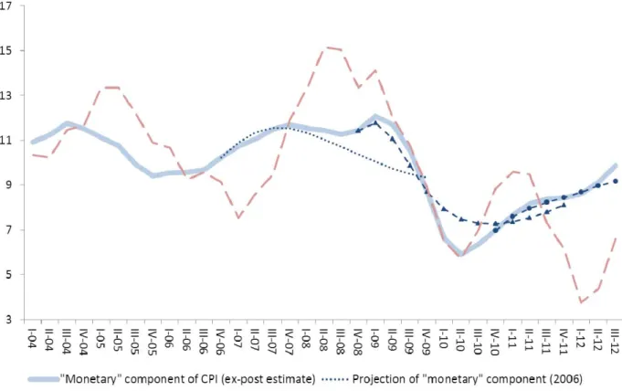
In order to illustrate this point, we extracted the underlying “monetary” part of inflation as the sum of the baseline projection and fluctuations caused by monetary shocks. The unconditional forecast of this component may be derived by extrapolating the baseline projection and estimating the residual effect of observed “monetary” shocks. Remarkably, over a considerably long horizon this projection will not deviate substantially from the ex-post estimate. This is because (as can be seen from Figure 1b) current “monetary” fluctuations of inflation are predetermined by past “monetary” shocks, while the contemporaneous shocks will only fully show in six to eight quarters. We produced several such unconditional projections recursively, i.e. only using shocks identified prior to the given period.12 We did this with a horizon of 12 quarters for the year ends of 2006 in the midst of on-going monetary expansion, 2008 after the first contractionary monetary shocks and 2010 when the monetary stance was returned to an accommodative level once again. The results indicate that based on the observed monetary developments, the underlying inflation trends could have been accurately projected, in particular for the next five to six quarters, namely the gradual increase and sharp drop of “monetary” CPI is correctly projected in 2006 and 2008 accordingly. The ex-post estimate of the “monetary” part of CPI in 2011 to 2012 seems to be fully in line with the projection produced at the end of 2010.

12_{Admittedly, estimating the whole model recursively might seem appropriate here. We did not do this for several}

reasons. Firstly, the aim of this exercise is to assess the leading properties of “monetary” shocks for inflation, not to test the model’s stability. Secondly, our time sample is too short for a fully recursive analysis; it seems crucial to have both phases of the monetary cycle (i.e. monetary expansion prior to 2008 and monetary contraction immediately after 2008) covered in the time sample and this would leave only the last few years of the sample available for the recursive analysis.

(17)

Figure 5. “Monetary” component of CPI (y-o-y growth, %)

5. Conclusions

Monetary analysis of inflationary risks is a potentially useful tool for monetary policy makers. Unfortunately this kind of analysis is often impeded by rapid financial developments that cause instability in some monetary instruments as well as substantial price shocks unrelated to monetary factors. It is therefore important to focus on low-frequency components in money growth and inflation when applying the monetary approach. Traditionally, these low frequency components are derived by smoothing the analysed variables over long time horizons. This method, however, may be less applicable to transition countries where time series are usually relatively short. Instead we employ an alternative approach for the identification of such an underlying process by extracting the common component from the set of money and price variables.

We set up a dynamic factor model in a state space representation which we estimated over the dataset comprising 10 monetary and nine price variables using Bayesian methods. Based on this model, we estimated the common part of the dataset’s fluctuations which we further decomposed into a number of structural shocks. Importantly, one of the shocks has empirical properties, in

(18)

terms of impulse response functions for example, that are fully in line with the theoretically expected money growth–inflation relationship, confirming that the process identified may have the capacity for economic interpretation. This process is relevant for the dynamics of CPI as well as other price indices, in particular for core inflation and housing prices.

Therefore, it is possible to separate the inflationary developments that are associated with changes in monetary stance from shorter-lived shocks. The results obtained indicate that monetary factors had an accelerating effect on inflation prior to the recent financial crisis and a restrictive effect after it. Inflation fluctuations associated with shocks to food and administered prices were correctly filtered out as non-monetary. Remarkably, the leading properties of monetary shocks for prices mean that the respective component of inflation may accurately be extrapolated based on the monetary developments observed.

(19)

References

Andrews, D.W.K. (1991) Heteroskedasticity and autocorrelation consistent covariance matrix estimation. Econometrica, 59, 817–858

Blake, A. and Mumtaz, H. (2012) Applied Bayesian econometrics for central bankers, CCBS Technical Handbook No. 4, Bank of England

Forni, M. and Gambetti, L. (2010) The dynamic effects of monetary policy: A structural factor model approach, Journal of Monetary Economics 57, 203–216

Forni, M., Giannone, D., Lippi, M. and Reichlin, L. (2009) Opening the black box: structural factor models with large cross-sections. Econometric Theory 25, 1319–1347

Forni, M., Hallin, M., Lippi, M. and Reichlin, L. (2000) The generalized dynamic factor model: identification and estimation, The Review of Economics and Statistics 82, 540–554.

Forni, M. and Lippi, M. (2001) The generalized dynamic factor model: representation theory. Econometric Theory 17, 1113–1141

Korhonen, I. and Mehrotra, A. (2010) Money demand in post-crisis Russia: de-dollarisation and re-monetisation, Emerging Markets Finance and Trade, 46 (2), 5 – 19

Mehrotra, A. and Ponomarenko, A. (2010) Wealth effects and Russian money demand, Discussion Paper Series, No. 13, BOFIT

Mumtaz, H., Solovyeva, A., and Vasilieva, E. (2012) Asset prices, credit and the Russian economy, Joint Research Paper No. 1, CCBS, Bank of England

Nicoletti-Altimari, S. (2001) Does money lead inflation in the euro area? Working Paper Series, No. 63, ECB

Nobili, A. (2009) Composite indicators for monetary analysis, Working Paper Series, No. 713, Bank of Italy

Oomes, N. and Ohnsorge, F. (2005) Money demand and inflation in dollarized economies: the case of Russia, Journal of Comparative Economics, 33(3), 462–483, September

Papademos, L.D. and Stark, J. (2010) Enhancing Monetary Analysis, ECB

Ponomarenko, A., Solovyeva, A. and Vasilieva, E. (2013) Financial dollarization in Russia: causes and consequences, Macroeconomics and Finance in Emerging Market Economies (forthcoming)

Ponomarenko, A., Vasilieva, E. and Schobert, F. (2012) Feedback to the ECB’s monetary

analysis: The Bank of Russia’s experience with some key tools, Working Paper Series, No. 1471, ECB

Stock, J.H. and Watson, M. (2011) Dynamic Factor Models, Oxford Handbook of Forecasting, Michael P. Clements and David F. Hendry (eds), Oxford University Press, Oxford

(20)

Uhlig, H. (2005) What are the effects of monetary policy on output? Results from an agnostic identification procedure, Journal of Monetary Economics 52, 381–419

(21)

Annex

Figure 6. Money series (y-o-y growth, %)

-20 0 20 40 60 04 05 06 07 08 09 10 11 12 M1_HH -20 0 20 40 60 04 05 06 07 08 09 10 11 12 M1_NFC -20 0 20 40 60 80 04 05 06 07 08 09 10 11 12 DEP_HH -40 0 40 80 120 160 04 05 06 07 08 09 10 11 12 DEP_NFC -40 0 40 80 120 04 05 06 07 08 09 10 11 12 DEPX_HH -100 0 100 200 300 400 500 04 05 06 07 08 09 10 11 12 DEPX_NFC -50 0 50 100 150 04 05 06 07 08 09 10 11 12 CASHX -20 0 20 40 60 04 05 06 07 08 09 10 11 12 M2 -20 0 20 40 60 04 05 06 07 08 09 10 11 12 DIV 0 10 20 30 40 50 04 05 06 07 08 09 10 11 12 M2X

Figure 7. Prices series (y-o-y growth, %)

0 4 8 12 16 04 05 06 07 08 09 10 11 12 CPI 4 6 8 10 12 14 16 04 05 06 07 08 09 10 11 12 Core 4 6 8 10 12 04 05 06 07 08 09 10 11 12 Non-food 0 5 10 15 20 25 04 05 06 07 08 09 10 11 12 Food 4 8 12 16 20 24 04 05 06 07 08 09 10 11 12 Inv 4 8 12 16 20 04 05 06 07 08 09 10 11 12 DA -10 0 10 20 30 04 05 06 07 08 09 10 11 12 GDP -10 0 10 20 30 40 50 04 05 06 07 08 09 10 11 12 HP I -20 0 20 40 60 04 05 06 07 08 09 10 11 12 HP II

(22)

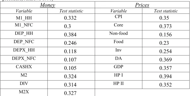
Table 3. Results of KPSS unit root test (the bandwidth is determined by the automatic Andrews procedure; Andrews 1991)