PDXScholar
Computer Science Faculty Publications and
Presentations
Computer Science
2014
A Comparative Study of Reservoir Computing for Temporal Signal
Processing
Alireza Goudarzi
University of New MexicoPeter Banda
Portland State University
Matthew R. Lakin
University of New MexicoChristof Teuscher
Portland State University, [email protected]
Darko Stefanovic
University of New MexicoLet us know how access to this document benefits you.
Follow this and additional works at:
http://pdxscholar.library.pdx.edu/compsci_fac
Part of the
Computer Engineering Commons
,
Numerical Analysis and Scientific Computing
Commons
, and the
Signal Processing Commons
This Pre-Print is brought to you for free and open access. It has been accepted for inclusion in Computer Science Faculty Publications and Presentations by an authorized administrator of PDXScholar. For more information, please [email protected].
Citation Details
Goudarzi, Alireza, et al. "A Comparative Study of Reservoir Computing for Temporal Signal Processing." arXiv preprint arXiv:1401.2224 (2014).
A Comparative Study of Reservoir Computing
for Temporal Signal Processing
Alireza Goudarzi
1, Peter Banda
2, Matthew R. Lakin
1, Christof Teuscher
3, and Darko Stefanovic
1Abstract—Reservoir computing (RC) is a novel approach to time series prediction using recurrent neural networks. In RC, an input signal perturbs the intrinsic dynamics of a medium called a reservoir. A readout layer is then trained to reconstruct a target output from the reservoir’s state. The multitude of RC architectures and evaluation metrics poses a challenge to both practitioners and theorists who study the task-solving performance and computational power of RC. In addition, in contrast to traditional computation models, the reservoir is a dynamical system in which computation and memory are inseparable, and therefore hard to analyze. Here, we compare echo state networks (ESN), a popular RC architecture, with tapped-delay lines (DL) and nonlinear autoregressive exogenous (NARX) networks, which we use to model systems with limited computation and limited memory respectively. We compare the performance of the three sys-tems while computing three common benchmark time series: H´enon Map, NARMA10, and NARMA20. We find that the role of the reservoir in the reservoir computing paradigm goes beyond providing a memory of the past inputs. The DL and the NARX network have higher memorization capability, but fall short of the generalization power of the ESN.
Index Terms—Reservoir computing, echo state networks, nonlinear autoregressive networks, time-delayed networks, time series computing
I. INTRODUCTION
Reservoir computing is a recent development in recur-rent neural network research with applications to temporal pattern recognition [1]. RC’s performance in time series processing tasks and its flexible implementation has made it an intriguing concept in machine learning and uncon-ventional computing communities [2]–[12]. In this paper, we functionally compare the performance of reservoir com-puting with linear and nonlinear autoregressive methods for temporal signal processing to develop a baseline for under-standing memory and information processing in reservoir computing.
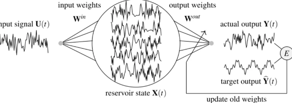
In reservoir computing, a high-dimensional dynamical core called areservoir is perturbed with an external input. The reservoir states are then linearly combined to create the output. The readout parameters can be calculated by performing regression on the state of a teacher-driven reservoir and the expected teacher output. Figure 1 shows a sample RC architecture. Unlike other forms of neural com-putation, computation in RC takes place within the transient
1Department of Computer Science, University of New Mexico,
Albu-querque, NM 87131, USA e-mail: [email protected].
2Department of Computer Science, Portland State University, Portland,
OR 97207, USA.
3 Department of Electrical and Computer Engineering, Portland State
University, Portland, OR 97207, USA.
dynamics of the reservoir. The computational power of the reservoir is attributed to a short-term memory created by the reservoir [13] and the ability to preserve the temporal information from distinct signals over time [14], [15]. Several studies attributed this property to the dynamical regime of the reservoir and showed it to be optimal when the system operates in the critical dynamical regime—a regime in which perturbations to the system’s trajectory in its phase space neither spread nor die out [15]–[19]. The reason for this observation remains unknown. Maass et al. [14] proved that given the two properties of sep-aration and approximation, a reservoir system is capable of approximating any time series. The separation property ensures that the reservoir perturbations from distinct signals remain distinguishable whereas the approximation property ensures that the output layer can approximate any function of the reservoir states to an arbitrary degree of accuracy. Jaeger [20] proposed that an ideal reservoir needs to have the so-called echo state property (ESP), which means that the reservoir states asymptotically depend on the input and not the initial state of the reservoir. It has also been sug-gested that the reservoir dynamics acts like a spatiotemporal kernel, projecting the input signal onto a high-dimensional feature space [5], [21]. However, unlike in kernel methods, the reservoir explicitly computes the feature space.
RC’s robustness to the underlying implementation as well as its efficient training algorithm makes it a suitable choice for time series analysis [22]. However, despite more than a decade of research in RC and many success stories, its wide-spread adoption is still forthcoming for three main reasons: first, the lack of theoretical understanding of RC’s working and its computational power, and second, the absence of a unifying implementation framework and per-formance analysis results, and thirdly, missing comparison with conventional methods.
II. OBJECTIVES
Our main objective is to compare time series computing in the RC paradigm, in which memory and computation are integrated, with two basic time series computing methods: first, a device with perfect memory and no computational power, ordinary linear regression on tapped-delay line (DL); and second, a device with limited memory and arbitrary computational power, a nonlinear autoregressive exogenous (NARX) neural network. This is a first step to-ward a systematic investigation of topology, memory, com-putation, and dynamics in RC. In this article we restrict our-selves to ESNs with a fully connected reservoir and input
reservoir stateX(t) Win input weights Wout output weights actual outputY(t) input signalU(t) target outputYb(t) E
update old weights
Figure 1. Computation in a reservoir computer. The reservoir is made up of a dynamical neural network with randomly assigned weights. The state of the nodes are represented byX(t). The input signalU(t)is fed into every reservoir nodeiwith a corresponding weightwin
i denoted with weight
column vectorWin= [win
i ]. Reservoir nodes are themselves coupled with each other using the weight matrixWres= [wresi j ], wherewresi j is the weight
of the connection from node jto nodei.
layer. We study the performance of ESN and autoregressive model on solving three time series problems: computing the 10th order NARMA time series [23], the 20th order NARMA time series [24], and the H´enon Map [25]. We also provide performance results using several variations of the mean squared error (MSE) and symmetric mean absolute percentage (SAMP) error to make our results accessible to the broader neural network and time series analysis research communities. Our systematic comparison between the ESN and autoregressive model provides solid evidence that the reservoir in the ESN performs non-trivial computation and is not just a memory device.
III. A BRIEFSURVEY OFPREVIOUSWORK The first conception of the RC paradigm in the recurrent neural network (RNN) community was Jaeger’s echo state network (ESN) [26]. In this early ESN, the reservoir consisted of N fully interconnected sigmoidal nodes. The reservoir connectivity was represented by a weight matrix with elements sampled from a uniform distribution in the interval [−1,1]. The weight matrix was then rescaled to have a spectral radius of λ <1, a sufficient condition for
ESP.
The input signal was connected to all the reservoir nodes and their weights were randomly assigned from the set {−1,1}. Later, Jaeger [20], [27] proposed that the
sparsity of the connection weight matrix would improve performance and therefore only 20% of the connections were assigned weights from the set {−47,47}.Verstraeten et al. [28] used a 50% sparse reservoir and a normal dis-tribution for the connection weights, and scaled the weight matrix posteriori to ensure the ESP; also, only 10% of the nodes were connected to the input. This study indicated that, contrary to the earlier report by Jaeger [26], the perfor-mance of the reservoir was sensitive to the spectral radius and showed optimality for λ≈1.1. Venayagamoorthy and
Shishir [29] demonstrated experimentally that the spectral radius also affects training time, but, they did not study spectral radii larger than one. Gallicchio and Micheli [30] provided evidence that the sparsity of the reservoir has a negligible effect on ESN performance, but depending on the
task, input weight heterogeneity can significantly improve performance. B¨using et al. [18] reported, from private communication with Jaeger, that different reservoir struc-tures, such as the scale-free and the small-world topologies, do not have any significant effect on ESN performance. Song and Feng [31] demonstrated that in ESNs, with complex network reservoirs, high average path length and low clustering coefficient improved the performance. This finding is at odds with what has been observed in complex cortical circuits [32] and other studies of ESN [33].
Rodan and Tino [24] studied an ESN model with a very simple reservoir consisting of nodes that are interconnected in a cycle with homogeneous input weights and homoge-neous reservoir weights, and showed that its performance can be made arbitrarily close to that of the classical ESN. This finding addressed for the first time concerns about the practical use of ESNs in embedded systems due to their complexity [2]. Massar and Massar [34] formulated a mean-field approximation to the ESN reservoir and demonstrated that the optimal standard deviation of a normally distributed weight matrix σw is an inverse power-law of the reservoir
size N with exponent −0.5. However, this optimality is
based on having critical dynamics and not task-solving performance.
IV. MODELS
To understand reservoir computation, we compare its behavior with a system with perfect memory and no com-putational power and a system with limited memory and arbitrary computational power.
We choose delay line systems, NARX neural networks, and echo state networks as described below. We useU(t),
Y(t), andYb(t)to denote the time-dependent input signals, the time dependent output signal, and the time-dependent target signal, respectively.
A. Delay line
A tapped-delay line (DL) is a simple system that allows us to access a delayed version of a signal. To compare the computation in a reservoir with the DL, we use a linear readout layer and connect it to read the states of
U(t)
b delay line stateX(t)
Wout
Y(t)
(a)
U(t)
b b
NARX delay line stateX(t)
Wout Y(t) (b) U(t) b reservoir stateX(t) Win Wout Y(t) (c) Figure 2. Architecture of delay line with a linear readout, the NARX neural network, and the ESN.
the DL. Figure 2(a) is a schematic for this architecture. Note that this architecture is different from the delay line used in [24] in that the input is only connected to a single unit in the delay line. The delay units do not perform any computation. The system is then fed with a teacher input and the weights are trained using an ordinary linear regression on the teacher output as follows:
Wout= (XT·X)−1·XT·Yb, (1)
where each row of X represents the state of the DL at a specific timeX(t0)and the rows ofYbare the teacher output at for the corresponding timeY(t0). Note that the DL states are augmented with a bias unit with a constant valueb=1. Initially, all the DL states are set to zero.
B. NARX Network
The NARX network is an autoregressive neural network architecture with a tapped delay input and one or more hidden layers. Both hidden layers and the output layer are provided with a bias input with constant valueb=1. We use tanh as the transfer function for the hidden layer and a linear transfer function for the output layer. The network is trained using the Marquardt algorithm [35]. This architec-ture performs a nonlinear regression on the teacher output using the previous values of the input accessible through the tapped delay line. A schematic of this architecture is given in Figure 2(b). Since we would like to study the effect of regression complexity on the performance, we fix the length of the tapped delay to 10 and vary the number of hidden nodes.
C. Echo State Network
In our ESN, the reservoir consists of a fully connected network of N nodes extended with a constant bias node
b=1. The input and the output nodes are connected to all the reservoir nodes. The input weight matrix is an I×N
matrixWin= [win
i,j], whereI is the number of input nodes
and win
j,i is the weight of the connection from input node
i to reservoir node j. The connection weights inside the reservoir are represented by anN×NmatrixWres= [wresj,k], where wres
j,k is the weight from node k to node j in the
reservoir. The output weight matrix is an(N+1(×Omatrix
Wout= [wout
l,k], whereOis the number of output nodes and
wout
l,k is the weight of the connection from reservoir nodekto
output nodel. All the weights are samples of i.i.d. random variables from a normal distribution with meanµw=0 and
standard deviationσw. We represent the time-varying input
signal by an Ith order column vector U(t) = [ui(t)], the
reservoir state by anNth order column vectorX(t) = [xj(t)],
and the generated output by an Oth order column vector Y(t) = [yl(t)]. We compute the time evolution of each
reservoir node in discrete time as:
xj(t+1) =tanh(Wresj ·X(t) +Win·U(t)), (2)
where tanh is the nonlinear transfer function of the reservoir nodes and Wres
j is the jth row of the reservoir weight
matrix. The reservoir output is then given by:
Y(t) =Wout·X(t). (3)
We train the output weights to minimize the squared output error E =||Y(t)−Yb(t)||2 given the target output Yb(t). As with DL, the output weights are calculated using the ordinary linear regression given in Equation 1.
V. EVALUATIONMETHODOLOGY
The study of task-solving performance and analysis of computational power in RC is a major challenge because there are a variety of RC architectures, each with a unique set of parameters that potentially affect the performance. The optimal RC parameters are task-dependent and must be adjusted experimentally. Furthermore, not all studies use the same tasks and the same performance metrics to evaluate their results. In addition, in contrast to classical computation models in which a programmed automaton acts on a storage device, RC is a dynamical system in which memory and computing are inseparable parts of a single phenomenon. In other words, in RC the same dynamical process that performs computation also retains the memory of the previous results and inputs. Thus, it is not clear how much of the RC’s performance can be attributed to its memory capacity and how much to its computational power. As a way of approaching this issue, we attempt to create a functional comparison between the ESN, DL, and NARX networks.
We choose three temporal tasks for our evaluation: the H´enon Map, the NARMA 10 time series, and the NARMA 20 time series. These tasks vary in increasing order in their
time lag dependencies and the number of terms involved and thus let us compare the performance of our systems based on the memory and computational requirements for task solving. We measure the performance using three variations of MSE and a SAMP error measure to allow easy comparison with related work.
A. Tasks
1) H´enon Map Time Series: This time series is generated by the following system:
yt=1−1.4y2t−1+0.3yt−2+zt, (4)
where zt is a white noise term with standard deviation
0.001. This is an example of a task that requires limited
computation and memory, and can therefore be used as a baseline to evaluate ESN performance.
2) NARMA 10 Time Series: Nonlinear autoregressive moving average (NARMA) is a discrete-time temporal task with 10th-order time lag. To simplify the notation we use
yt to denotey(t). The NARMA 10 time series is given by:
yt=αyt−1+βyt−1 n
∑
i=1 yt−i+γut−nut−1+δ, (5) where n =10, α =0.3,β =0.05,γ =1.5,δ =0.1. Theinput ut is drawn from a uniform distribution in the
interval [0,0.5]. This task presents a challenging problem to any computational system because of its nonlinearity and dependence on long time lags. Calculating the task is trivial if one has access to a device capable of algorithmic programming and perfect memory of both the input and the outputs of up to 10 previous time steps. This task is often used to evaluate the memory capacity and computational power of ESN and other recurrent neural networks.
3) NARMA 20 Time Series: NARMA 20 requires twice the memory and computation compared to NARMA 10 with an additional nonlinearity because of the saturation functiontanh. This task is very unstable and the saturation function keeps its values bounded. NARMA 20 time series is given by: yt=tanh(αyt−1+βyt−1 n
∑
i=1 yt−i+γut−nut−1+δ), (6)wheren=20, and the rest of the constants are set as in NARMA 10.
B. Error Calculation
A challenge in comparing results across different studies is the way each study evaluates its results. In the case of time series analysis, each study may use a different error calculation to measure the performance of the presented methods. We present three different error calculations com-monly used in the time series analysis literature. We use
y to refer to the time-dependent output and by to refer to the target output. The expectation operatorh·irefers to the
time average of its operand.
1) Root normalized mean squared error: The most commonly used measure is a root normalized mean squared error (RNMSE) calculated as follows:
RNMSE= s
h(y−by)2i
σbyw2
. (7)
Here σby2 is the standard deviation of the target output
over time. In some studies this calculation is used without taking the square root, in which case it is simply called a normalized mean squared error (NMSE).
2) Normalized root mean squared error: A variant of the normalized error is the normalized root mean square error (NRMSE), also known as normalized root mean squared deviation (NRMSD). It is calculated as follows:
NRMSE= p
h(y−by)2i
max(by)−min(by). (8) In this variant, the error is normalized by the width of the range covered by the target signal. Both RNMSE and NRMSE attempt to normalize the error between 0 and 1. However, if the distance between the output and the target output is larger than the standard deviation of the target output or its range, they may produce an error value larger than 1.
3) Symmetric absolute mean percentage error: The symmetric absolute mean percentage (SAMP) error, on the other hand, is guaranteed to produce an error value between 0% and 100%. SAMP is given by:
SAMP=100× |y− b y| y+by . (9)
Throughout the rest of the paper, we use the RNMSE er-ror to produce the plots and make our comparison between the three systems. We have tabulated the results using the other metrics in the Appendix B.
C. Reservoir optimization
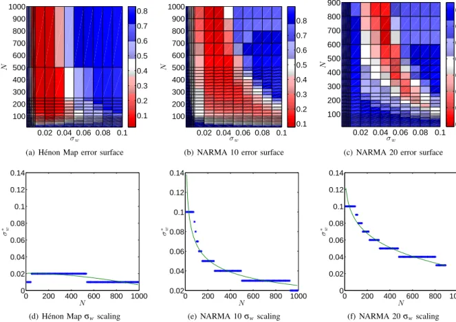
Depending on the ESN architecture, its performance can be sensitive to some of the model’s parameters. These pa-rameters are optimized using offline cross-validation [24], [36] or online adaptation [19], [37]. This is a preliminary stage before the functional comparison. We are interested in the scaling of these parameters, which we study systemat-ically. Figures 3(a)-3(c) shows the resulting error surface by averaging the result of the 10 runs of each σw-N
combination. We observe that, as the nonlinearity of the task and its required memory increase, ESN performance becomes more sensitive to changes inσwand favors a more
heterogeneous weight assignment (largerσw). We find the
optimal standard deviationσw∗ as a function ofN for each
task:
σw∗(N) =arg min
σw
RNMSE(σw,N). (10)
We found experimentally that σw∗(N) is best fitted by a
power-law curve. The bottom row of Figure 3 shows the result of this optimization and the power-law fit. The details of these fits are provided in Appendix A. For NARMA 10
0.02 0.04 0.06 0.08 0.1 100 200 300 400 500 600 700 800 900 1000 σw N 0.1 0.2 0.3 0.4 0.5 0.6 0.7 0.8
(a) H´enon Map error surface
0.02 0.04 0.06 0.08 0.1 100 200 300 400 500 600 700 800 900 1000 σw N 0.1 0.2 0.3 0.4 0.5 0.6 0.7 0.8
(b) NARMA 10 error surface
0.02 0.04 0.06 0.08 0.1 100 200 300 400 500 600 700 800 900 σw N 0.2 0.3 0.4 0.5 0.6 0.7 0.8 0.9
(c) NARMA 20 error surface
0 200 400 600 800 1000 0 0.02 0.04 0.06 0.08 0.1 0.12 0.14 σ ∗ w N
(d) H´enon Mapσwscaling
0 200 400 600 800 1000 0.02 0.04 0.06 0.08 0.1 0.12 0.14 σ ∗ w N
(e) NARMA 10σwscaling
0 200 400 600 800 1000 0 0.02 0.04 0.06 0.08 0.1 0.12 0.14 σ ∗ w N (f) NARMA 20σwscaling
Figure 3. Scaling and optimization in the ESN. Figures 3(a), 3(b), and 3(c) show the training error surface of the ESN on the H´enon Map, the NARMA 10, and the NARMA 20 tasks respectively. We create a scaling-law by finding the optimal standard deviationσw∗(N)according to Equation 10 and
fitting the power-lawaxb+cto it. Figures 3(d), 3(e), and 3(f) show the data points (blue markers) and the fit (solid line) for theσ∗
w(N).
and NARMA 20 the power law is well behaved, except for the H´enon Map which is not sensitive to σw. We use σw∗=0.02 for H´enon Map experiments. It is noteworthy
that this power-law behavior is qualitatively consistent with what we expect from the theoretical result in [34], although the exact power-law coefficient is task-dependent.
D. Functional Comparison
The division between memory and computation is not fully understood. Here, we attempt to compare the ESN size to the size of an equivalent device with only memory capacity and no computational power, and to a device with limited memory and theoretically arbitrary computational power. A DL of length nstores the perfect memory of the past n inputs and a NARX network with N hidden units can be a universal approximator of any time series. We would like to compare the performance of a linear readout with access to the reservoir state with a linear readout with access to the delay line states and also to the performance of the NARX network. It is clear that the ESN, the DL, and the NARX network are very different, i.e., the memory and computational power of ESN, DL, and NARX networks differ significantly even with identical N. Therefore, we perform a functional comparison in which we study the ESN, the DL, and the NARX network with equal RNMSE
on the same task. For ESN, we have two parameters: the standard deviation of the normal distribution used to create the weight matrix σw and the number of nodes N in the
reservoir. We chose theσw that optimizes the performance
of ESN for each N as described in Section V-C.
E. Experimental Setup
In this section we describe the parameters and data sets used for our simulations. The training and testing for delay line and NARX networks are done by generating 10 time series of 4,000 time steps. We used 20 time seres of the same length for ESNs. We used the first 2,000 time steps of each time series to train the model and the second 2,000 steps to test the model. The training and testing performance metrics are then averaged over the 10 runs. The model specific setting are as follows:
1) Delay line: A delay line is a fixed system with only one parameterN that defines the number of taps. For this study we limit ourselves to 1≤N≤2,000. We have also
experimented with 2,000≤N≤3,000, but the performance
of the delay line does not change for N>2,000. We take
N=2,000 as the largest delay line for this study.
2) NARX neural network: Since the training in the NARX network is sensitive to the random initial weights, we instantiate a new network for each time series. We fix
0 500 1000 1500 2000 0 0.1 0.2 0.3 0.4 0.5 0.6 0.7 0.8 0.9 1 Normalized size RNMSE Delay line NARX NN ESN
(a) H´enon Map training
0 500 1000 1500 2000 0 0.1 0.2 0.3 0.4 0.5 0.6 0.7 0.8 0.9 1 Normalized size RNMSE Delay line NARX NN ESN (b) NARMA 10 training 0 500 1000 1500 2000 0 0.1 0.2 0.3 0.4 0.5 0.6 0.7 0.8 0.9 1 Normalized size RNMSE Delay line NARX NN ESN (c) NARMA 20 training 0 500 1000 1500 2000 10−5 100 105 1010 Normalized size RNMSE Delay line NARX NN ESN
(d) H´enon Map generalization
0 500 1000 1500 2000 10−5 100 105 1010 Normalized size RNMSE Delay line NARX NN ESN
(e) NARMA 10 generalization
0 500 1000 1500 2000 10−5 100 105 1010 Normalized size RNMSE Delay line NARX NN ESN (f) NARMA 20 generalization
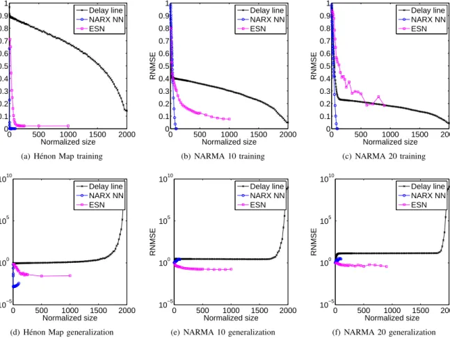
Figure 4. Training and generalization RNMSE of the DL, the NARX network, and the ESN for three different tasks. The DL can memorize the patterns, but not generalize for any of the tasks. The NARX network can generalize for the H´enon Map, but overfits for the NARMA 10 and the NARMA 20. The ESN can both memorize and generalize the temporal patterns for all the tasks.
the number of input taps to 10 and the number of hidden layers to 1. We use the number of nodes in the hidden layer
N as the control parameter, with 1≤N≤100.
3) Echo state network: A single instantiation of ESN contains randomly assigned weights and the reservoir initial states. To average the ESN properties over these variations we instantiate five ESN to train and test for every time series. The error is then averaged over the five instances and then over 20 time series. The variable parameters for ESN are the number of reservoir nodesNand the standard deviation of the normal distribution used to generate the reservoir and the input weights. However, for each N we only use theσw∗as described in Section V-C. We study the
ESN with the reservoir size 10≤N≤1,000.
VI. RESULTS
Figures 4(a)-4(c) show the training performance mea-sured in RNMSE as a function of the normalized system size. In all three tasks, the delay line shows a sharp decrease in error as soon as the system acquires enough capacity to hold all the required information for the task. This is
N=2 for H´enon Map,N=10 for NARMA 10 task, and
N=20 for NARMA 20 task. After this point, the error decreases slowly until N=2,000 where RNMSE≈0.14
after a sharp drop. The decrease in error is due to the
“dimensionality curse”: the fixed-length teacher time series are not representatives of the expanded state space of the delay line. This is expected to result in overfitting, which is reflected in the high testing errors on Figures 4(d)-4(f). Another expected behavior of overfitting to training data is that if the distribution of the data is wide, the error will be larger and for narrower distributions of data the error will be lower. This is why the delay line has the highest error for the simplest task, the H´enon Map, and the lowest error for the most difficult task, the NARMA 20 task. Note that to make the testing errors for all the system readable, we use logarithmic y-axes.
The NARX network behaves differently on the H´enon Map and the two NARMA tasks. For the H´enon Map, it shows the best training and testing performance aroundN= 5 and begins to overfits for N>5. For both NARMA 10
and NARMA 20, the training error decreases gradually as the number of hidden nodes increases, but the system only memorizes the patterns and cannot generalize, which is characterized by increasing test RNMSE. For the NARMA 10 task, the observed training RNMSE for NARX network is comparable to the error of 0.17 reported by Atiya and
Parlos [23] for the same network size N=40. However, they used only 200 data points, which explains the slightly lower error. Atiya and Parlos focused on the convergence
times of different algorithms and did not publish their testing error.
For the ESN, the training error on all three tasks de-creases rapidly as the size of the reservoir inde-creases and reaches a plateau forN≈1,000. However, unlike the DL
and the NARX network, the testing error also decreases sharply as the reservoir size increases. As expected, this decrease is sharper for easier tasks. The main different of the ESN performance is that the training error increases across allN as the difficulty of the task increases, which is a sign that the readout layer is not merely memorizing the training patterns. We have tabulated the error values for all three systems on all the tasks for a few system sizes, which can be found in the Appendix B. Our ESN testing results are similar to those reported by Rodan and Tino [24] for the same system size.
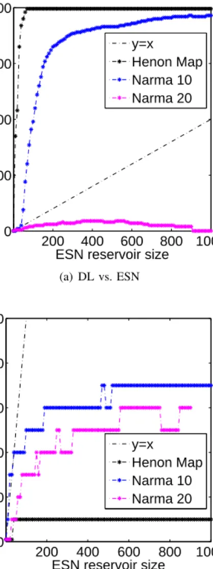
Next, we compared the performance of the DL, the NARX network, and the ESN as described in Section V-D. Because the testing error of the systems do not overlap, we have to use the training error to perform a direct functional comparison between the three systems. This allows us to compare their memorization capabilities. Figure 5(a) shows the DL size as a function of the ESN size of identical training error for all three tasks. For the H´enon Map and the NARMA 10 tasks, the ESN achieves the same RNMSE as the delay line with significantly fewer nodes. For instance for the H´enon Map and NARMA 10, to achieve a training RNMSE of an ESN with 400 nodes, a delay line would need 1,990 and 1,810 nodes respectively. For NARMA
20, the delay line only needs 90 nodes to achieve the same RNMSE as an ESN with 400 nodes. The narrow distribution of the NARMA 20 time series allow the linear delay line to exploit the average case strategy to achieve a lower RNMSE. On the other hand, the ESN readout layer learns the task itself as in contrast to just memorizing patterns. The delay line use the same strategy for the easier tasks as well (NARMA 10 and H´enon Map), but ESN can fit to the the training data much better than the delay line and therefore requires much less resources to achieve the same error level.
Figure 5(b) shows the functional comparison result be-tween NARX networks and ESNs. A NARX network would need 10 hidden nodes to achieve the same RNMSE as a 400-node ESN on the H´enon Map task. The short time dependency and the simple form of this task make it very easy for the network to learn the system, which results in low training and testing RNMSE. For the NARMA 10 and the NARMA 20 tasks, the network requires 60 and 50 hidden nodes to be equivalent of the 400-node ESN. The strategy here is similar to the delay line where during learning the network tries to fit the training data on average, as best as it can. As expected this strategy will have two consequences: (1) the NARMA 20 task will be easier because of its distribution; (2) the network overfits the training data and cannot generalize to testing data.
VII. DISCUSSION ANDOPENPROBLEMS The reservoir in an ESN is a dynamical system in which memory and computation are inseparable. To understand this type of information processing we compared the ESN performance with a memory-only device, the DL, and a limited-memory but computationally powerful device, the NARX network. Our results illustrate that the performance of ESN is not only due to its memory capacity; ESN read-out does not create an autoregression of the input, such as in the DL or the NARX network. The information processing that takes place inside a reservoir is fundamentally different from other types of neural networks. The exact mecha-nism of this process remains to be investigated. Studying reservoir computing usually takes place by analyzing the systems performance for task solving with different
com-200 400 600 800 1000 0 500 1000 1500 2000
ESN reservoir size
Delay line size
y=x Henon Map Narma 10 Narma 20 (a) DL vs. ESN 200 400 600 800 1000 0 20 40 60 80 100
ESN reservoir size
NARX NN hidden layer size
y=x Henon Map Narma 10 Narma 20
(b) NARX NN vs. ESN
Figure 5. Figure 5(a) shows how the complexity of the DL compares with the ESN of identical memorization performance. Except for the NARMA 20, which requires perfect memory of the 20 previous time steps, the ESN memorization capability far surpasses the DL. Figure 5(b) shows the same comparison between the NARX and the ESN. The NARX network out performs the ESN in all tasks. Due its complexity, the NARX network can memorize the patterns very well, but is not able to generalize to the new patterns (see Figure 4).
putational and memory requirements. To understand the details of information processing in a reservoir, we have to understand the effects of the reservoir’s architecture on its fundamental memory and computational capacity. We also have to be able to define the classes of tasks that can be parametrically varied in memory requirement and nonlinearity. Our study reveals that although ESN cannot memorize patterns as well as a memory device or a neural network, it greatly outperforms them in generalizing to novel inputs. Also, increasing reservoir size in ESN improves the performance of generalization, whereas in the DL or the NARX network this will result in increased over-fitting leading to poorer generalization. One solution would be to extend the receiver operation characteristic (ROC) and receiver error characteristic (REC) curve methods to decide on the quality of generalization in ESN [38]–[40]. In the neural network community, methods based on pruning, regularization, cross-validation, and information criterion have been used to alleviate the overfitting problem [41]– [53]. Among these methods, regularization has been suc-cessfully used in ESNs [3]. However, these methods focus on increasing the neural network’s performance and are not suitable to quantify overfitting or to study task hardness. Another area that requires more research is the amount of training that the ESN requires to guarantee a certain performance, as is described in probably approximately correct methods [54]–[56]. To the best of our knowledge these problems have not been addressed in the case of high-dimensional dynamical systems. A well developed theory of computation in reservoir computing needs to address all of these aspects. In future work, we will study some of these issues experimentally and based on our observations, we will attempt to develop theoretical understanding of computation in the reservoir computing paradigm.
VIII. CONCLUSION
Reservoir computing is an approach to neural network training which has been successful in areas of machine learning, time series analysis, robot control, and sequence learning. There has been many studies aimed at under-standing the working of RC and the factors that affect its performance. However, because of the complexity of the reservoir in RC, none of these studies have been completely satisfactory and have often resulted in contradictory con-clusions. In this paper, we compared the performance of three approaches to time series analysis: the delay line, the NARX network, and the ESN. These methods vary in their memory capacity and computational power. The delay line retains a perfect memory of the past, but does not have any computational power. The NARX network only has limited memory of the past, but in principle can perform any computation. Finally, the ESN does not have an explicit access to past memory, but its reservoir carries out computation using the implicit memory of the past represented in its dynamics. Using a functional comparison we showed that for simple tasks with short time dependencies, the delay line requires more than four
times as much resources that ESN requires to achieve the same error, while the NARX network requires 40 times less resources than ESN to achieve equivalent error. For tasks with long time dependencies and narrow distributions the delay line requires less than one fourth the resources of the ESN and the NARX network requires less then one fifth the same resources. However, neither a delay line nor a NARX network can achieve the generalization power of an ESN. Many theoretical aspects of reservoir computing, such as the memory-computation trade-off, and the relation between reservoir’s structure, its dynamics, and its performance remain as open problems.
ACKNOWLEDGMENT
The work was support by NSF grants #1028238 and #1028120. M.R.L. gratefully acknowledges support from the New Mexico Cancer Nanoscience and Microsystems Training Center.
APPENDIXA FITTINGσw
Before we can fit σw∗, we have to interpolate the data
points on the error surface with a linear fit. This allows us to use all values of N and σw and create a smooth fit.
Table I shows the goodness of fit statistics for the linear fit to the error surface. Low SSE and high R2 statistics on this fit shows the the surface accurately represent the data points. We then calculate theσw∗corresponding to the
task SSE R2
H´enon Map 1.5486×10⁻³¹ 1
NARMA 10 2.989×10⁻³¹ 1
NARMA 20 7.3725×10⁻³¹ 1
Table I
GOODNESS OF FIT STATISTICS FOR THE INTERPOLANT FIT TO THE
ERROR SURFACE(FIGURE3)AS A FUNCTION OF RESERVOIRσwANDN
FOR ALL THREE TASKS.
standard deviation of the weight matrix for each N that minimizes the error. We represent σw∗ as a function of N
and fit the power-lawaxb+cto it. The result of the fit and
the goodness of fit statistics are given in Table II. APPENDIXB
THEPERFORMANCERESULTS
Tables III, IV, and V tabulate the average testing and training errors of optimal ESNs, delay lines, and NARX networks for the three different tasks using three different measures, i.e., RNMSE, NRMSE, and SAMP.
REFERENCES
[1] B. Schrauwen, D. Verstraeten, and J. V. Campenhout, “An overview of reservoir computing: theory, applications and implementations,”
inProceedings of the 15th European Symposium on Artificial Neural
Networks, 2007, pp. 471–482.
[2] D. Prokhorov, “Echo state networks: appeal and challenges,” in
Neural Networks, 2005. IJCNN ’05. Proceedings. 2005 IEEE
In-ternational Joint Conference on, vol. 3, 2005, pp. 1463–1466 vol.
task measure N=50,σw∗=0.02 N=100,σw∗=0.02 N=150,σw∗=0.02 N=200,σw∗=0.02 N=500,σw∗=0.02
H´enon Map
RNMSE trainingtesting 00..24743805±±00..07380215 00..10530385±±00..00390225 00..04480247±±00..00610008 00..03590230±±00..00480002 00..02640226±±00..00010026 NRMSE trainingtesting 00..06961071±±00..02080060 00..02960109±±00..00110063 00..01260069±±00..00170002 00..01010065±±00..00140000 00..00740063±±00..00000007 SAMP trainingtesting 1616..27976023±±11..20461912 33..24700074±±00..38994199 11..41822687±±00..15771440 00..97978498±±00..06720584 00..94416821±±00..03730527 task measure N=50,σw∗=0.10 N=100,σw∗=0.07 N=150,σw∗=0.05 N=200,σw∗=0.05 N=500,σw∗=0.04 NARMA 10
RNMSE trainingtesting 00..38964035±±00..00700073 00..32703036±±00..01040113 00..25602300±±00..00640058 00..21991904±±00..00540051 00..17961248±±00..00560078 NRMSE trainingtesting 00..06350653±±00..00110012 00..05290495±±00..00170018 00..04140374±±00..00110010 00..03550309±±00..00090008 00..02910202±±00..00090013 SAMP trainingtesting 44..61377961±±00..08620819 33..82975742±±00..13431467 22..88276224±±00..08810742 22..40241247±±00..07190642 11..97104310±±00..06540900 task measure N=50,σw∗=0.10 N=100,σw∗=0.09 N=150,σw∗=0.08 N=200,σw∗=0.07 N=500,σw∗=0.04
NARMA 20
RNMSE trainingtesting 00..78468003±±00..02460257 00..53135746±±00..04990510 80.6177.4478±±240..06502443 50.7683.4171±±130..06210557 00..38732776±±00..01830222 NRMSE trainingtesting 00..09851012±±00..00320031 00..07280667±±00..00650062 10..06620562±±20..96470082 00..72600524±±10..64340078 00..04910349±±00..00230028 SAMP trainingtesting 23..95070570±±00..08300776 22..37361860±±00..19221874 61..08119531±±70..75392518 15..36908459±±70..23492461 11..81343097±±00..08070965
Table III
TRAINING AND TESTING ERRORS FOR THE OPTIMALESNON THREE DIFFERENT TASKS MEASURED USING THREE DIFFERENT ERROR METRICS
RNMSE, NRMSE,ANDSAMP. THE OPTIMALσw∗IS MEASURED USING THERNMSEON THE TRAINING DATA. EACH DATA POINT IS AVERAGED
OVER100EXPERIMENTS.
task measure N=100 N=200 N=500 N=1000 N=2000
H´enon Map
RNMSE trainingtesting 00..91648726±±00..00440051 00..93788478±±00..00380037 01..02437848±±00..01200049 10..22946764±±00..01830060 133054723910..14265757±±09380091076.0066 .0147 NRMSE trainingtesting 00..24522581±±00..00170011 00..26362382±±00..00170009 00..28862208±±00..00370018 00..34631901±±00..00110046 37487476540..47920402±±26461554540.0018 .1636
SAMP trainingtesting 5756..86350839±±00..35923953 5854..35111909±±00..36982825 5059..47231493±±00..58853639 6042..97607874±±00..56504785 952..53022081±±00.1497.4781
task measure N=100 N=200 N=500 N=1000 N=2000
NARMA 10
RNMSE trainingtesting 20..91503972±±00..01881827 20..90883884±±00..01931852 02..87973590±±00..19190224 20..80633017±±00..21520230 10071032720..04979273±±0482045875.0072 .2627 NRMSE trainingtesting 00..46420650±±00..00210360 00..46330635±±00..00200363 00..45860586±±00..03700021 00..44680493±±00..04010025 1640911250..00821086±±083497086.0013 .3948
SAMP trainingtesting 274.6786.5133±±01..16600130 274..58244396±±01.1747.0251 274.2474.2029±±01..19700782 263..59895114±±01..25752347 1000.1873.0000±±00.0222.0000
task measure N=100 N=200 N=500 N=1000 N=2000
NARMA 20
RNMSE trainingtesting 130.2620.5807±±00..00937275 130..22896650±±00.0068.7321 130.2132.7338±±00..00667514 130..18049180±±00..00917712 12345603670..04506547±±0811645432.0061 .8192 NRMSE trainingtesting 01..03337237±±00..03820020 01..73460290±±00..04020014 10..74330271±±00..04290014 10..76670229±±00..00170457 1603916180..48660057±±1097099160.0007 .7516
SAMP trainingtesting 431.3211.8473±±00..08555246 441..15330038±±00.0600.5579 441.0761.1198±±00..06155911 440..89804313±±00..07436170 1000.1113.0000±±00.0132.0000
Table IV
TRAINING AND TESTING ERRORS FOR THE DELAY LINE RESERVOIR ON THREE DIFFERENT TASKS MEASURED USING THREE DIFFERENT ERROR
METRICSRNMSE, NRMSE,ANDSAMP. EACH DATA POINT IS AVERAGED OVER10EXPERIMENTS.
task measure N=5 N=10 N=30 N=50 N=100
H´enon Map
RNMSE trainingtesting 00..00140014±±00..00000000 00..00150013±±00..00000000 00..00160012±±00..00000000 00..00190011±±00..00010000 00..00370009±±00..00000008 NRMSE trainingtesting 00..00040004±±00..00000000 00..00040004±±00..00000000 00..00050003±±00..00000000 00..00050003±±00..00000000 00..00100003±±00..00000002 SAMP trainingtesting 00..19002091±±00..02930304 00..19141692±±00..02920218 00..21101674±±00..02940293 00..23231455±±00..03540140 00..32631098±±00..01420335
NARMA 10
RNMSE trainingtesting 01..90810894±±00..00740072 01..16278235±±00..00910121 10..53635010±±00..02330094 01..93222450±±00..03300100 20..50150000±±00..00000755 NRMSE trainingtesting 00..26173156±±00..00300018 00..33682373±±00..00280048 00..44511444±±00..00800026 00..55980706±±00..01100028 00..72460000±±00..00000227 SAMP trainingtesting 3026..46462977±±00..31684856 3124..95132035±±00..34645791 1740..43120853±±00..89232634 4710..15033269±±00..69354612 520..00007679±±01.0000.0017
NARMA 20
RNMSE trainingtesting 01..92762201±±00..27340046 01..44588468±±00..00635060 10..55945279±±00..02380100 02..06892725±±00..05800084 20..86660000±±00..00000921 NRMSE trainingtesting 00..26733538±±00..08060015 00..41892441±±00..00221466 00..45171521±±00..00770030 00..59940785±±00..01860026 00..83070000±±00..00000310 SAMP trainingtesting 3026..42136541±±00..28406264 3124..97257928±±00..24427206 1740..29416939±±00..79372953 4711..88710069±±00..84874056 540..00005926±±01.0000.1815
Table V
TRAINING AND TESTING ERRORS FOR THENARXNETWORK ON THREE DIFFERENT TASKS MEASURED USING THREE DIFFERENT ERROR METRICS
RNMSE, NRMSE,ANDSAMP. EACH DATA POINT IS AVERAGED OVER10EXPERIMENTS.
[3] F. Wyffels and B. Schrauwen, “A comparative study of reservoir computing strategies for monthly time series prediction,”
Neurocom-puting, vol. 73, no. 10–12, pp. 1958–1964, 2010.
[4] H. Jaeger, “Adaptive nonlinear system identification with echo state networks,” inNIPS, 2002, pp. 593–600.
H´enon Map SSE 0.0011 R2 0.5670 a −5.733×10⁻⁸±2.9430×10⁻⁷ b 1.795±0.7450 c 0.02053±0.0016 NARMA 10 SSE 2.9686×10⁻⁴ R2 0.9926 a 0.306±0.0095 b −0.2609±0.0249 c −0.02537±0.0079 NARMA 20 SSE 5.8581×10⁻⁴ R2 0.9909 a −0.03441±0.0143 b 0.2156±0.0408 c 0.1766±0.0210 Table II
GOODNESS OF FIT STATISTICS FOR THE POWER-LAW FITaxb+cTOσ∗
w
(FIGURE3)AS A FUNCTION OF RESERVOIR SIZENFOR ALL THREE
TASKS.
recurrent neural network training,”Computer Science Review, vol. 3, no. 3, pp. 127–149, 2009.
[6] H. O. Sillin, R. Aguilera, H.-H. Shieh, A. V. Avizienis, M. Aono, A. Z. Stieg, and J. K. Gimzewski, “A theoretical and experimental study of neuromorphic atomic switch networks for reservoir com-puting,”Nanotechnology, vol. 24, no. 38, p. 384004, 2013. [7] M. Fiers, B. Maes, and P. Bienstman, “Dynamics of coupled cavities
for optical reservoir computing,” in Proceedings of the 2009
An-nual Symposium of the IEEE Photonics Benelux Chapter, S. Beri,
P. Tassin, G. Craggs, X. Leijtens, and J. Danckaert, Eds. VUB Press, 2009, pp. 129–132.
[8] G. Indiveri, B. Linares-Barranco, R. Legenstein, G. Deligeorgis, and T. Prodromakis, “Integration of nanoscale memristor synapses in neuromorphic computing architectures,” Nanotechnology, vol. 24, no. 38, p. 384010, 2013.
[9] O. Obst, A. Trinchi, S. G. Hardin, M. Chadwick, I. Cole, T. H. Muster, N. Hoschke, D. Ostry, D. Price, K. N. Pham, and T. Wark, “Nano-scale reservoir computing,”Nano Communication Networks, vol. 4, no. 4, pp. 189–196, 2013.
[10] Y. Paquot, F. Duport, A. Smerieri, J. Dambre, B. Schrauwen, M. Haelterman, and S. Massar, “Optoelectronic reservoir comput-ing,”Scientific Reports, vol. 2, 02 2012.
[11] C. Fernando and S. Sojakka, “Pattern recognition in a bucket,” in
Advances in Artificial Life, ser. Lecture Notes in Computer Science,
W. Banzhaf, J. Ziegler, T. Christaller, P. Dittrich, and J. Kim, Eds. Springer Berlin Heidelberg, 2003, vol. 2801, pp. 588–597. [12] A. Goudarzi, M. R. Lakin, and D. Stefanovic, “DNA reservoir
computing: A novel molecular computing approach,” inDNA
Com-puting and Molecular Programming, ser. Lecture Notes in Computer
Science, D. Soloveichik and B. Yurke, Eds. Springer International Publishing, 2013, vol. 8141, pp. 76–89.
[13] H. Jaeger and H. Haas, “Harnessing nonlinearity: Predicting chaotic systems and saving energy in wireless communication,”Science, vol. 304, no. 5667, pp. 78–80, 2004.
[14] W. Maass, T. Natschl¨ager, and H. Markram, “Real-time computing without stable states: a new framework for neural computation based on perturbations,”Neural Computation, vol. 14, no. 11, pp. 2531–60, 2002.
[15] T. Natschl¨ager and W. Maass, “Information dynamics and emergent computation in recurrent circuits of spiking neurons,” in Proc. of
NIPS 2003, Advances in Neural Information Processing Systems,
S. Thrun, L. Saul, and B. Schoelkpf, Eds., vol. 16. Cambridge: MIT Press, 2004, pp. 1255–1262.
[16] N. Bertschinger and T. Natschl¨ager, “Real-time computation at the edge of chaos in recurrent neural networks,”Neural Computation, vol. 16, no. 7, pp. 1413–1436, 2004.
[17] D. Snyder, A. Goudarzi, and C. Teuscher, “Computational capabil-ities of random automata networks for reservoir computing,”Phys.
Rev. E, vol. 87, p. 042808, Apr 2013.
[18] L. B¨using, B. Schrauwen, and R. Legenstein, “Connectivity, dynam-ics, and memory in reservoir computing with binary and analog neurons.”Neural Computation, vol. 22, no. 5, pp. 1272–1311, 2010. [19] J. Boedecker, O. Obst, N. M. Mayer, and M. Asada, “Initialization and self-organized optimization of recurrent neural network connec-tivity,”HFSP Journal, vol. 3, no. 5, pp. 340–349, 2009.
[20] H. Jaeger, “Tutorial on training recurrent neural networks, covering BPPT, RTRL, EKF and the “ echo state network” approach,” German National Research Center for Information Technology, St. Augustin-Germany, Tech. Rep. GMD Report 159, 2002.
[21] M. Hermans and B. Schrauwen, “Recurrent kernel machines: Com-puting with infinite echo state networks,” Neural Computation, vol. 24, no. 1, pp. 104–133, 2013/11/22 2011.
[22] M. Lukoˇseviˇcius, H. Jaeger, and B. Schrauwen, “Reservoir comput-ing trends,”KI - K¨unstliche Intelligenz, vol. 26, no. 4, pp. 365–371, 2012.
[23] A. Atiya and A. Parlos, “New results on recurrent network train-ing: unifying the algorithms and accelerating convergence,”Neural
Networks, IEEE Transactions on, vol. 11, no. 3, pp. 697–709, 2000.
[24] A. Rodan and P. Tino, “Minimum complexity echo state network,”
Neural Networks, IEEE Transactions on, vol. 22, no. 1, pp. 131–144,
2011.
[25] M. H´enon, “A two-dimensional mapping with a strange attractor,”
Communications in Mathematical Physics, vol. 50, no. 1, pp. 69–77,
1976.
[26] H. Jaeger, “The “echo state” approach to analysing and training recurrent neural networks,” St. Augustin: German National Research Center for Information Technology, Tech. Rep. GMD Rep. 148, 2001.
[27] ——, “Short term memory in echo state networks,” GMD-Forschungszentrum Informationstechnik, Tech. Rep. GMD Report 152, 2002.
[28] M. D. D. Verstraeten, B. Schrauwen and D. Stroobandt, “An experimental unification of reservoir computing methods,”Neural
Networks, vol. 20, no. 3, pp. 391–403, 2007.
[29] G. K. Venayagamoorthy and B. Shishir, “Effects of spectral radius and settling time in the performance of echo state networks,”Neural
Networks, vol. 22, no. 7, pp. 861 – 863, 2009.
[30] C. Gallicchio and A. Micheli, “Architectural and markovian factors of echo state networks,”Neural Networks, vol. 24, no. 5, pp. 440 – 456, 2011.
[31] Q. Song and Z. Feng, “Effects of connectivity structure of complex echo state network on its prediction performance for nonlinear time series,”Neurocomputing, vol. 73, no. 10–12, pp. 2177 – 2185, 2010. [32] E. Bullmore and O. Sporns, “Complex brain networks: graph theoret-ical analysis of structural and functional systems,”Nat Rev Neurosci, vol. 10, no. 4, pp. 312–312, 04 2009.
[33] S. Dasgupta, P. Manoonpong, and F. Woergoetter, “Small world topology of dynamic reservoir for effective solution of memory guided tasks,”Frontiers in Computational Neuroscience, no. 177. [34] M. Massar and S. Massar, “Mean-field theory of echo state
net-works,”Phys. Rev. E, vol. 87, p. 042809, Apr 2013.
[35] M. Hagan and M.-B. Menhaj, “Training feedforward networks with the marquardt algorithm,”Neural Networks, IEEE Transactions on, vol. 5, no. 6, pp. 989–993, 1994.
[36] H. Jaeger, M. Lukoˇseviˇcius, D. Popovici, and U. Siewert, “Optimiza-tion and applica“Optimiza-tions of echo state networks with leaky- integrator neurons,”Neural Networks, vol. 20, no. 3, pp. 335–352, 2007. [37] S. Dasgupta, F. Wrgtter, and P. Manoonpong, “Information theoretic
self-organised adaptation in reservoirs for temporal memory tasks,”
inEngineering Applications of Neural Networks, ser.
Communica-tions in Computer and Information Science, C. Jayne, S. Yue, and L. Iliadis, Eds. Springer Berlin Heidelberg, 2012, vol. 311, pp. 31–40.
[38] J. Bi and K. P. Bennett, “Regression error characteristic curves.” in
ICML, T. Fawcett and N. Mishra, Eds. AAAI Press, 2003, pp. 43–50.
[39] W. Waegeman, B. De Baets, and L. Boullart, “A comparison of different ROC measures for ordinal regression,” in Proceedings of the 3rd International Workshop on ROC Analysis in Machine
Learning., N. Lachiche, C. Ferri, and S. Macskassy, Eds., 2006, pp.
63–69.
[40] ——, “ROC analysis in ordinal regression learning,”Pattern Recogn.
Lett., vol. 29, no. 1, pp. 1–9, Jan. 2008.
inNeural Networks for Signal Processing, 1992. II., Proceedings of
the 1992 IEEE Workshop on, 1992, pp. 29–38.
[42] J. Larsen, C. Svarer, L. Andersen, and L. Hansen, “Adaptive regu-larization in neural network modeling,” inNeural Networks: Tricks
of the Trade, ser. Lecture Notes in Computer Science, G. Orr and
K.-R. Mller, Eds. Springer Berlin Heidelberg, 1998, vol. 1524, pp. 113–132.
[43] J. Larsen, L. Hansen, C. Svarer, and M. Ohlsson, “Design and reg-ularization of neural networks: the optimal use of a validation set,”
inNeural Networks for Signal Processing, 1996. VI. Proceedings of
the 1996 IEEE Workshop on, 1996, pp. 62–71.
[44] J. Larsen and L. Hansen, “Empirical generalization assessment of neural network models,” inNeural Networks for Signal Processing,
1995. V. Proceedings of the 1995 IEEE Workshop on, 1995, pp.
30–39.
[45] ——, “Generalization performance of regularized neural network models,” inNeural Networks for Signal Processing, 1994. IV.
Pro-ceedings of the 1994 IEEE Workshop on, 1994, pp. 42–51.
[46] S. Lawrence, C. L. Giles, and A. C. Tsoi, “Lessons in neural network training: Overfitting may be harder than expected,” inIn Proceedings of the Fourteenth National Conference on Artificial Intelligence,
AAAI-97. AAAI Press, 1997, pp. 540–545.
[47] N. Murata, S. Yoshizawa, and S.-I. Amari, “Network information criterion-determining the number of hidden units for an artificial neural network model,” Neural Networks, IEEE Transactions on, vol. 5, no. 6, pp. 865–872, 1994.
[48] J. Moody, “Prediction risk and architecture selection for neural networks,” in From Statistics to Neural Networks, ser. NATO ASI Series, V. Cherkassky, J. Friedman, and H. Wechsler, Eds. Springer Berlin Heidelberg, 1994, vol. 136, pp. 147–165.
[49] L. K. Hansen and C. E. Rasmussen, “Pruning from adaptive reg-ularization,” Neural Computation, vol. 6, no. 6, pp. 1223–1232, 2013/12/11 1994.
[50] B. R. Stallard and J. G. Taylor, “Quantifying multivariate classifica-tion performance: the problem of overfitting,” pp. 426–436, 1999. [51] D. M. Hawkins, “The problem of overfitting,”Journal of Chemical
Information and Computer Sciences, vol. 44, no. 1, pp. 1–12, 2004.
[52] E. Baum and D. Haussler, “What size net gives valid generalization?”
Neural Computation, vol. 1, no. 1, pp. 151–160, 1989.
[53] B. Amirikian and H. Nishimura, “What size network is good for generalization of a specific task of interest?”Neural Networks, vol. 7, no. 2, pp. 321–329, 1994.
[54] M. Kearns, Y. Mansour, D. Ron, R. Rubinfeld, R. E. Schapire, and L. Sellie, “On the learnability of discrete distributions,” in
Proceedings of the Twenty-sixth Annual ACM Symposium on Theory
of Computing, ser. STOC ’94. New York, NY, USA: ACM, 1994,
pp. 273–282.
[55] R. Lange and R. M¨anner, “Quantifying a critical training set size for generalization and overfitting using teacher neural networks,” in
ICANN ’94, M. Marinaro and P. G. Morasso, Eds. Springer London,
1994, pp. 497–500.
[56] L. Valiant, “A theory of the learnable,”Communications of the ACM, vol. 27, no. 11, pp. 1134–1142, 1984.