Collaborative Motion Planning

(1)

COLLABORATIVE MOTION PLANNING

A Dissertation by

JORY LONDON DENNY

Submitted to the Office of Graduate and Professional Studies of Texas A&M University

in partial fulfillment of the requirements for the degree of DOCTOR OF PHILOSOPHY

Chair of Committee, Nancy M. Amato Committee Members, Suman Chakravorty

Dylan Shell Dezhen Song Head of Department, Dilma da Silva

August 2016

Major Subject: Computer Science

(2)

ABSTRACT

Planning motion is an essential component for any autonomous robotic system. An intelligent agent must be able to efficiently plan collision-free paths in order to move through its world. Despite its importance, this problem is PSPACE-Hard which means that even planning motions for simple robots is computationally difficult. State-of-the-art approaches trade completeness (always able to provide a solution if one exists or report none exists) for probabilistic completeness (probabilistically guaranteed to find a solution if one exists but cannot report if none exists) and improved efficiency. These methods use sampling-based techniques to design a se-quence of motions for the robot. However, as these methods are random in nature, the probability of their success is directly related to the expansiveness, or openness, of the underlying planning space. In other words, narrow passages, complex systems, and various constraints make planning with these methods difficult. On the other hand, humans can often determine approximate solutions for these difficult solutions quickly.

In this research, we explore user-guided planning in which a human operator works together with a sampling-based motion planner. By having a human-in-the-loop, a human can steer a sampling-based planner towards a solution. This strategy can provide benefits to many applications such as computer-aided design and virtual prototyping, to name a few.

We begin by classifying and creating simple models of common user-guided and heuristic-guided motion planning methods. Our models encompass three forms of user input: configuration-based, path-based, and region-based input. We compare and contrast these approaches and motivate our choice of a region-based collaborative

(3)

framework. Through this analysis, we gain insight into user-guided planning and further motivate methods that harness low interface complexity and work entirely in workspace, which is most natural to a human operator. Further, we extend the theory of expansiveness to analyze the various types of user inputs.

Our novel region-based collaboration framework takes advantage of human intu-ition by allowing a user to define regions in the workspace to bias and/or constrain the search space of a sampling-based motion planner. This approach allows a user to bias a high dimensional search with low dimensional input, supports intermittent user hints, and empowers a user to customize motion solutions.

Finally, we extend region steering to both non-holonomic robotic systems and a human-inspired approach to motion planning.

Our results show that this region-based framework can aid many variants of sampling-based planning, reduce computation time, support solution customization, and can be used to develop advanced heuristic methods for solving motion planning problems. We provide experiments exemplifying our approach in planning motions for complex robotic applications such as mobile manipulators, car-like, and free-flying robots.

(4)

DEDICATION

To Katelynn, Pippin, and everyone near and far who supports me through my lifes adventure.

(5)

ACKNOWLEDGEMENTS

The research contained in this dissertation and my entire graduate career would not have become a reality without the help of colleagues, friends, and family. You have my sincerest gratitude, and I apologize if I left key players out of the acknowl-edgements, it was not my intention. This research was also supported in part by a National Science Foundation (NSF) Graduate Research Fellowship (GRFP).

To my advisor, Dr. Nancy M. Amato, I would like to thank you most for your continual advice and support. Since, I started undergraduate research in January 2009, I have come to you for professional advice and attribute many of my successes and awards to you. Specifically, completing my undergraduate thesis, being a fi-nalist for the Computing Research Associations (CRA) Outstanding Undergraduate Research award, earning a NSF GRFP, numerous departmental awards, experiences abroad at conferences, helping me to become an Assistant Professor at the Univer-sity of Richmond, and now my Ph.D. degree can be traced back to many helpful meetings. I look forward to many future years of advice and collaboration.

To my committee, Dr. Suman Chakravorty, Dr. Dylan Shell, and Dr. Dezhen Song, thank you for conversations at conferences, challenges during my preliminary and final exams, and your support in various endeavors throughout the past few years.

To my future colleagues, Dr. Kostas Bekris, Dr. Dilma da Silva, Dr. Dan Halperin, Dr. Jason O’Kane, and Dr. Lydia Tapia, thank you for professional support and letters of recommendation from which I earned an NSF GRFP and became an Assistant Professor at the University of Richmond.

(6)

Read Sandstr¨om, undergraduate students Nicole Julian, Brennen Taylor, Andrew Bregger, and Ben Smith, and high school students Jonathan Colbert, Brandon Mar-tinez, Hongsen Qin, and Eli Zamora, thank you for your help on the research con-tained within this dissertation. Without you, it would have taken much longer, if at all, to complete.

To my collaborators on other projects and friends within the Parasol Lab, I sincerely enjoyed working with you all during my graduate studies and appreciate the fun experiences we shared in lab. I would specifically like to thank Ali-akbar Agha-mohammadi, Chinwe Ekenna, Mukulika Ghosh, Andrew Giese, Adam Fidel, Aditya Mahadevan, Dr. Samuel Rodriguez, Read Sandstr¨om, Dr. Timmie Smith, Brennen Taylor, Dr. Shawna Thomas, and Hsin-Yi (Cindy) Yeh.

To my friends inside and outside of the Parasol Lab and to the friendships which did not last, thank you. Each friend, past and present, has taught me something and always shaped my life for the better. I want to specifically name Andrew Giese, Nancy Luong, Zachary Pollock, Brennen Taylor, and Shawn Vicknair, who always manage to stay in contact and support me. I am forever grateful.

To my mom, Barbara, and dad, Gerald, I have not always been the perfect son and have often been distant, but I want to thank you for loving me and supporting me unconditionally. You never said “no” to my endeavors and you never told me that I had to be anyone else than who I was. I love you and I am proud to be your son.

To my brother, Jason, we have had our differences throughout our lives and have never been much for words, but I want to thank you for being a constant source of motivation and let you know that I could not have imagined having a better brother. I love you.

(7)

much I love you, but I do. You brought so much joy to my final years of graduate school. You are the perfect dog.

To my wife, Katelynn, I love you more than anything else in the world. You are beautiful and an endless supply of love. You always provide the perfect distraction from the stresses of life, which allows me to remain calm, patient, and resolved. I love all the smiles, laughter, and joy you bring to my life each and every day. I look forward to the next stage of our lives!

(8)

3. USER-GUIDED PLANNING . . . 26

(9)

3.1.1 Configuration-based Input . . . 27

3.1.2 Path-based Input . . . 27

3.1.3 Region-based Input . . . 28

3.2 Experimental Analysis of User Input Modalities . . . 28

3.2.1 Setup . . . 29

3.2.2 Results . . . 30

3.3 Discussion . . . 33

4. REGION-BASED COLLABORATIVE PLANNING . . . 34

4.1 Framework . . . 34

4.1.1 Overview . . . 35

4.1.2 User Input . . . 39

4.1.3 Completeness . . . 41

4.2 Framework Variants . . . 42

4.2.1 Collaborative Region-biased Roadmap Construction . . . 42

4.2.2 Collaborative Region-biased Tree Construction . . . 44

4.2.3 Collaborative Region-biased Hybrid Methods . . . 45

4.3 Experimental Analysis of Variants . . . 46

4.3.1 Setup . . . 46

4.3.2 Region-biased PRM . . . 48

4.3.3 Region-biased RRT . . . 51

4.3.4 Region-biased Spark PRM . . . 52

4.4 Experimental Analysis of Collaboration Loop . . . 54

4.4.1 Setup . . . 54

4.4.2 Results . . . 58

4.5 Experimental Analysis of Roadmap Customization . . . 61

5. ON THE THEORY OF USER-GUIDED PLANNING . . . 64

5.1 Determining Cf ree Parameters . . . 64

5.1.1 ǫ . . . 64

5.1.2 β . . . 65

5.2 Analysis of User-guided Planning . . . 67

5.2.1 Configuration-based Input . . . 67 5.2.2 Path-based Input . . . 69 5.2.3 Region-based Input . . . 70 6. KINODYNAMIC REGION-BIASED RRT . . . 72 6.1 State Space . . . 72 6.2 Algorithmic Modifications . . . 72 6.3 Experimental Analysis . . . 74 6.3.1 Setup . . . 74

(10)

6.3.2 Analysis . . . 75 7. DYNAMIC REGION-BIASED RRT . . . 78 7.1 Algorithm . . . 78 7.1.1 Embedding Graph . . . 79 7.1.2 Flow Graph . . . 81 7.1.3 Region-biased RRT Growth . . . 82 7.1.4 Example . . . 82 7.2 Experimental Analysis . . . 83 7.2.1 Setup . . . 85 7.2.2 Discussion . . . 85 8. CONCLUSION . . . 88 REFERENCES . . . 90

(11)

LIST OF FIGURES

FIGURE Page

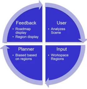
1.1 Overview of Product Lifecycle Management (PLM). Figure adapted

from [102]. . . 2

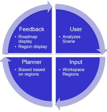
1.2 Overview of our region-based collaborative framework. . . 5

2.1 Region examples. . . 11

2.2 Configuration q and its visibility set V(q) (red). . . 18

2.3 Set X (red) and its β–lookout(green). . . 20

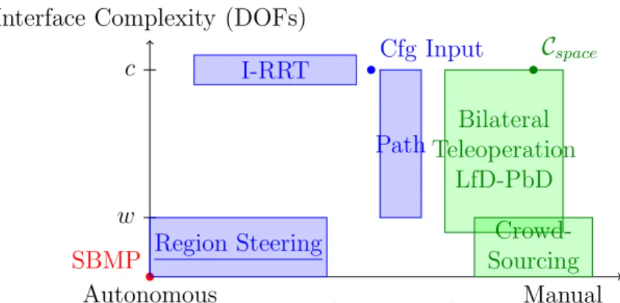
2.4 Interface complexity in terms of degrees of freedom manipulated versus level of autonomy in expected behavior, where c is the degrees of freedom of theCspaceand wis the degrees of freedom of the workspace is shown. The approach described in Chapter 4, called Region Steering here (underlined), is a combination of high autonomy mixed with a simple interface. . . 23

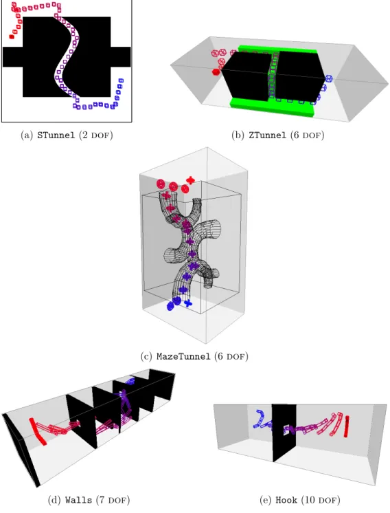
3.1 Test scenarios. The start (solid red) to end (hollow blue) of an example solution path is shown. . . 31

3.2 Experimental results for building a roadmap without user-input (PRM), configuration-based input (Cfg), path-based input (Path), and region-based input (Region). (a) Number of nodes, (b) number of CD Calls, and (c) time in seconds to solve the representative query averaged over ten trials are shown. . . 32

4.1 Alpha puzzle. A pathologically difficult motion planning problem in which the two α shaped peices must be separated. . . 35

4.2 In one direction, the user specifies workspace regions, and in the other direction, the planner displays the current progress in planning. . . . 36

(12)

4.3 Example scenario. (a) A user pre-specifies one avoid and two attract regions. (b) An attract region is shaded red to indicate declining usefulness. (c) The user responds by moving the region to a more productive location. (d) The resulting roadmap. . . 38 4.4 A user has drawn a region to mark the narrow passage and set the

sampler to OBPRM [2] in the region. Region-biased PRM uses this to bias roadmap construction to the narrow passage. . . 43 4.5 A user has drawn a region to act as a waypoint for the RRT, influencing

Region-biased RRT to grow through the narrow passage. . . 45 4.6 A user has created a region to mark a narrow passage and

Region-biased Spark PRM begins growing a RRT within. . . 46 4.7 Example scenarios used in experimental analysis. (a) A planar 2 dof

scenario. (b) An 8dofmobile manipulator. All queries require traver-sal through narrow passages between the start (solid red) and goal (hollow blue) configurations. . . 48 4.8 Speedups of various PRM construction methods compared with a

tuned Gaussian PRM (Gaussian-T). . . 49 4.9 Speedup of various RRT techniques compared with RRT. . . 52 4.10 Speedup comparison between Region-biased Spark PRM and Spark

PRM. . . 53 4.11 Various environments for experimental analysis. All queries require

traversal through narrow passages between the start (solid red) and goal (hollow blue) configurations. . . 57 4.12 (a) Number of nodes, and (b) time required by each method to solve

the construction query, normalized to OBPRM. For the Region-biased PRM methods in (b), the upper portion of the bar represents the user’s pre-specification time, while the lower portion represents the time taken by the automated planner after pre-specification. . . 59 4.13 (a) Building and (b) Helicopter environments used to illustrate

roadmap customizability. Avoidance regions are shown in dark gray and queries are shown as solid red/hollow blue pairs. . . 62

(13)

5.1 E (red line) is the set of configurations with the smallest visibility ra-tio. V(E) is shown in transparent red. E∗ _{is shown as a configuration} in blue. Notice thatE∗ _{has an equivalent visibility to} _E_{. . . .} ₆₅ 5.2 B (green line) is the set of configurations that are part of the smallest

maximalβ–lookouts across all ofCf ree. Configurationsqa,qb, qc are representative configurations that have a small maximalβ–lookout, their visibility sets are shown in transparent red. B∗ _{is shown in blue.} Notice that B∗ _{has an equivalent visibility to} _B_. _{. . . .} ₆₆ 5.3 Configurations placed on E∗ _and _B∗ _{that represent}

configuration-based input that can help a sampling-configuration-based motion planner. The visibility regions of each configuration are shown, notice how they act as “beacons” for the space making the problem “easier.” . . . 68 6.1 Example scenarios used in experimental analysis. (a) A non-holonomic

robot with 3 positional dofs in a planar environment (6-dimensional state space). (b) A non-holonomic robot with 6 positional dofs in a volumetric environment (12-dimensional state space). All queries require traversal through narrow passages between the start (solid red) and goal (hollow blue) configurations. . . 75 6.2 Average running times and standard deviations for non-holonomic

ex-periments. For Planar, Region-biased RRT exhibits reduced mean planning time with a p-value of 0.0064 for a one-tailed t-test. For

Tunnel, the difference is more dramatic with a p-value of 0.0001. . . 76 7.1 Example execution of Dynamic Region-biased RRT: (a) environment;

(b) precomputed embedding graph (magenta) in workspace; (c) flow graph (magenta) computed from the start position; (d) initial region (green) placed at the source vertex of the flow graph; (e) Region-biased RRT growth (blue); and (f) multiple active regions (green) guiding the tree (blue) among multiple embedded arcs of the flow graph (magenta). . . 84 7.2 MazeTunnel environment. Note how there are false passages in the

workspace in which the robot cannot pass through. . . 86 7.3 On-line planning time comparing Dynamic Region-biased RRT with

(14)

LIST OF TABLES

TABLE Page

3.1 Success rates of experimental methods. . . 30

4.1 Success rates of various PRM construction methods. . . 49

4.2 Success rates of various RRT construction methods. . . 51

4.3 Success rates for Region-biased Spark PRM and Spark PRM. . . 53

4.4 Success rates for the various PRMs in the test environments. . . 58

4.5 Percentage of maps with shortest paths correctly steering away from the avoidance regions. . . 62

(15)

1. INTRODUCTION

The human mind is a powerful problem solving tool. Many domains leverage this by combining automation with human guidance. Robotics is no exception as both teleoperation [38] and user-guided motion planners, e.g., [45, 8, 59, 94, 102], have been developed to explore these synergies over the past few decades.

Our study focuses on motion planning, or the problem of finding a valid (e.g., collision-free) path for a robot among various robot and/or obstacle constraints. Motion planning has application in robotics, virtual reality [7, 64, 65, 83, 82], bioin-formatics [90, 5, 4, 92, 91, 95], and computer-aided design [8, 59, 94, 102], among others.

Over the past few decades, many approaches have been proposed to solve the motion planning problem. Early research classified the general problem in the com-plexity class PSPACE-Hard [81], which implies there is little hope to find an efficient, complete algorithm for this problem — acomplete algorithm will find a solution to a problem if one exists or report ‘NO’ if none exists. In fact, the best known complete algorithm is exponential in the complexity of the robot [13]. Most variants of the motion planning problem are equally difficult. Thus, research has explored other avenues for success, one of which is combining automated algorithms with human guidance.

A specific application that illustrates the potential benefit of combining user-guidance and motion planning is Product Lifecycle Management (PLM), shown in Figure 1.1, which is the process of design, implementation, and maintenance of prod-ucts. Motion planning can be used in a few portions of PLM. First, in the design phase, virtual prototyping could be used to validate constraints of possible designs.

(16)

Figure 1.1: Overview of Product Lifecycle Management (PLM). Figure adapted from [102].

Planning is important here to make sure the product can be maintained properly, i.e., parts can be replaced. Second, planning is often found in the manufacturing of products as robots are often used to make products. Third, in the service phase motion planning can be used in determining how to maintain the product. If user in-put/assistance can be incorporated into PLM, then these phases can be made better and/or more efficient and ultimately cheaper. For example, if user-guided planning is incorporated directly in a computer-aided design tool, then an engineer can validate constraints of the design in a cheap and efficient manner as compared with creating expensive and time consuming physical mock-ups of the product. There are specific challenges to designing a collaborative planner for these applications: (1) collabora-tion should occur seamlessly in real-time, (2) a user should provide “good” input to

(17)

aid the planner — “good” input will aid the planner in identifying the most difficult portions of a planning problem, (3) the planner should plan as close to real-time as possible, and (4) the planner should provide quality feedback on the effectiveness of the user input. This dissertation proposes a novel framework designed to address these challenges and constraints.

There are numerous automated approaches to motion planning. State-of-the-art automated techniques solve this problem through sampling-based methods [53, 43, 61]. These techniques approximate the free planning space by building random graphs, often called roadmaps, that contain representative feasible paths for the robot. As an example, Probabilistic RoadMaps (PRMs) [53], randomly sample the entire planning space and connect nearby samples together to form a roadmap. The map can then be queried for paths through the space by first connecting the start and goal configurations to the roadmap, and then by performing a single-source shortest path search in the graph, e.g., A∗ _{[33]. However, it is known that these} sampling-based techniques lack efficiency in the presence of narrow passages and difficult robot constraints [42, 52, 40, 43, 58, 41]. In these scenarios, research has aimed at developing intelligent approaches which bias sampling, e.g., [2, 11, 24, 21, 71], yet there are still problems which are difficult to solve efficiently.

User-guided planners encompass methodologies to limit the search space of the planner through user input. By specifying a presumably important (or unimportant) portion of the space, the user enables the planner to focus on a particular subset of the planning problem. Previous user-guided planners address this difficulty by attempting to harness the power of human intuition [45, 8, 59, 94, 102]. In these systems, the human often performs a global scene analysis of the workspace, while the machine handles high-precision tasks such as collision detection and low level path-finding [48, 32]. Recent work has explored sampling-based planning strategies that

(18)

incorporate interactive and collaborative planning techniques [94]. These approaches are restricted both to specific sampling-based planners and to an interface which can fully control the robot. To date, no one has come up with theoretically grounded methods for incorporating user input in a planner to solve problems cooperatively, which is the focus of this dissertation.

This dissertation addresses the challenges of providing an effective collaboration mechanism that (1) allows simple user input (not dependent on the complexity of the robot), (2) can work with any sampling-based motion planner, and (3) provides for efficient and effective collaboration and planning. Further, we develop and analyze the theoretical foundations of user-guided planning leading to a deeper understanding of how much and when user-input aids a sampling-based motion planner.

1.1 Research Contribution

In this work, we first seek to classify, model, and compare common user-guided approaches. We classify methods based upon the types of input they gather from the user. In this research, we focus on region-based approaches as they have a good trade-off between interface complexity and performance impact.

We introduce a region-based framework (Figure 1.2), in which a user can collab-oratively interact with a sampling-based planner by specifying a workspace region for the planner to prefer or avoid. In turn, this planner can inform the user of its progress and how useful the regions are to the user. Our framework maintains prob-abilistic completeness of the automated planner used. We show how this framework can be extended for common variants of sampling-based planning.

Our framework is demonstrated in an interactive system that requires only in-termittent user action on a standard computer interface, e.g., a mouse. The goal of this work is to understand how these hints and cooperation affect sampling-based

(19)

Figure 1.2: Overview of our region-based collaborative framework.

planning. The analysis and optimization of the user interface is the subject of future study.

We analyze each of the user input modalities. To do this, we expand on the con-cept of expansiveness [41] to theoretically analyze the impact these modalities have on the planning process. Our results indicate two things for each user-input modal-ity. First, we define conditions for each user-input method for when the input will aid a sampling-based motion planner. Second, we show that when these conditions are met, the user-input will make a motion planning problem “easier” and lead to more efficient planning for a sampling-based planner.

We show how this region-based framework can be extended to handle complex robot constraints such as non-holonomic constraints, e.g., car-like robots, and how the user-strategies seen in region steering can inspire a novel automated planning approach using geometric techniques for scene analysis.

(20)

• classification, modeling, and analysis of three types of user-guided input modal-ities: namely configuration-based, path-based, and region-based input,

• a generic region-based framework for collaborating with any sampling-based planner,

• a theoretical analysis of various user-guided input modalities quantifying both when user input aids in planning and proving that input will make the problem “easier” for a sampling-based motion planner,

• variants of our framework geared toward specific sampling-based planning paradigms, non-holonomic constraints, and a novel human-inspired approach to motion planning,

• and experimental validation of the aforementioned theoretic and algorithmic developments.

Portions of this research were previously published. The basic framework was presented as Region Steering in the proceedings of the Eleventh Workshop on the Algorithmic Foundations of Robotics (WAFR) [27]. The variants of our framework applied to graph-based, tree-based, and hybrid sampling-based planning approaches were published in the proceedings of the Seventeenth International Symposium on Robotics Research (ISRR) [26]. The discussions of user-guidance input models and theoretical impact of user-guidance on sampling-based motion planning were pub-lished in the proceedings of the International Conference on Intelligent Robots and Systems (IROS) [25].

1.2 Outline

Chapter 2 discusses important foundational knowledge in representing robots, configuration space, and current approaches to solving the motion planning problem.

(21)

Chapter 3 categorizes, models, and compares existing user-guided motion planning algorithms to motivate the algorithmic decisions taken in our region-based user-guidance. Our region-based framework is presented in Chapter 4, and we discuss extensions of the framework to three common paradigms of sampling-based plan-ning: graph-based, tree-based, and hybrid approaches. We revisit the various user input strategies and introduce the concept of augmented (ǫ′_, _α′_, _β′_{)–expansiveness} as a means to theoretically study the models in Chapter 5. Then we delve into two interesting extensions of our framework. First in Chapter 6, we extend our frame-work for handling non-holonomic constraints. Second in Chapter 7, we discuss an automated approach inspired from the user-guidance seen in our approach. Finally, we conclude and discuss future work in Chapter 8.

(22)

2. PRELIMINARIES AND RELATED WORK

In this chapter, we discuss motion planning preliminaries and relevant related work.

2.1 Preliminaries

In this section, we discuss preliminary definitions of modeling motion planning problems, and we discuss a few of the basic building blocks for sampling-based motion planning algorithms.

2.1.1 Motion Planning

A robot is a movable object whose position and orientation can be described byn

parameters, ordegrees of freedom (dofs), each corresponding to an object component (e.g., object positions, object orientations, link angles, and/or link displacements). The following definitions provide the formal specification of this placement, called a

configuration (Definition 2.1.1), and the set of all placements, called theconfiguration space (Cspace) [67] (Definition 2.1.2).

Definition 2.1.1. A configuration is a unique placement of the movable object in an environment. It is described by a point q = hx1, x2, ..., xni in an n-dimensional

space (where xi is the ith dof).

Definition 2.1.2. Theconfiguration space (Cspace)is the set of all configurations, feasible or not.

The Cspace may be partitioned into two subsets, free space (Cf ree) and obstacle space (Cobst), Definition 2.1.3 and Definition 2.1.4 respectively. The boundary be-tween the two subsets is referred to as the contact space and is denoted by ∂Cobst (Definition 2.1.5).

(23)

Definition 2.1.3. The free space (Cf ree) is the subset of all feasible configurations in Cspace.

Definition 2.1.4. The obstacle space (Cobst) is the union of all infeasible config-urations in Cspace. It can be described as Cspace\ Cf ree.

Definition 2.1.5. The contact space (∂Cobst) is the boundary of Cobst.

In general, it is infeasible to compute Cspace explicitly [81, 13], but we can often determine the validity of a single configuration quite efficiently, e.g., by performing a collision detection test in the workspace, the robot’s natural space. Validity is often defined as collision-free (i.e., avoiding both self-collision and collision with the environment) but can be generalized to other constraints such as closure constraints for closed chain systems [60] or energy requirements for computational biology ap-plications [90, 5, 4, 92, 91, 95].

Using the configuration space abstraction, the motion planning problem becomes that of finding a continuous trajectory in Cf ree from a given start configuration to a goal configuration or region.

2.1.2 Local Transitions

Often in motion planning, we are concerned with proximity between two config-urations, which is measured by a distance metric (Definition 2.1.6). Many metrics are possible, e.g., Euclidean, Manhattan, or Minkowski distances, and ideally should approximate the cost of transitioning between two configurations. In other words, a lower distance should represent an easier transition between the two configurations. Definition 2.1.6. A distance metric δ(q1, q2) measures the distance between two

(24)

When two configurations can be connected by a simple path, these configurations are said to be visible to each other. Visibility is checked by a local planner that returns a sequence of configurations such that all are inCf reeand the distance between consecutive configurations is below some resolution threshold or reports that no path is found. Local planners are often deterministic and must either be recomputable or stored. While in principle any local planner can be used, Definition 2.1.7 describes a common strategy, a straight-line interpolation through Cspace, that is also used in this work.

Definition 2.1.7. Two configurations q1 and q2 are visible if q1q2 ∈ Cf ree, where

q1q2 is a straight-line interpolation in Cspace. Let Visible(q1, q2) be a function which

verifies this constraint up to a particular environmental resolution, referred to as a

local planner.

Other common local planners include rotate-at-s[3] (which translates a configu-ration to a specified percentage, s, of its path towards its goal, rotates it, and then completes the translation to the goal), A∗ _{[33], and Toggle Local Planning [23] (which} performs local planning in a 2-dimensional triangular subspace of Cspace).

We define a sequence of local transitions as a path (Definition 2.1.8).

Definition 2.1.8. Two configurationsqi andqj are adjacent if δ(qi, qj)≤r, where r

is an environmental resolution. ApathΠ ={q1, q2, . . . , qm}is a continuous sequence

of adjacent configurations.

2.1.3 Regions

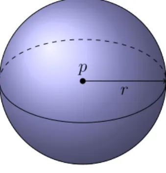
We define a region as any bounded volume in the workspace (Definition 2.1.9). Two common examples are axis-aligned bounding boxes (AABBs) and bounding spheres (BSs), shown in Figure 2.1.

(25)

p1

p2

(a) Axis-Aligned Bounding Box

p r

(b) Bounding Sphere Figure 2.1: Region examples.

Definition 2.1.9. A region R is any bounded volume in the workspace.

The usage of bounding volumes is not unique to motion planning and can be found in many fields. For example, collision detection libraries use bounding volumes to expedite validity checking of configurations [66].

“Region” can also be seen as a very broad term. A region might be seen as a path or constraint in the workspace to bias planning in Cspace. For example, one could imagine selecting a wall as a contact-constraint for an end-effector of an articulated robot. There are many possibilities, and we selected a few representative and simple region types for our study.

2.2 Sampling-based Motion Planning

Because of the cost of explicitly computing Cspace [81, 13], research has turned to sampling-based techniques to efficiently explore Cf ree for valid paths. These meth-ods generally fall under two classes: graph-based approaches, e.g., Probabilistic RoadMaps (PRMs) [53], and tree-based approaches, e.g., Rapidly-exploring Ran-dom Trees (RRTs) [61] or Expansive Space Trees (ESTs) [43].

(26)

Algorithm 1 Probabilistic RoadMap (PRM) Construction Input: A Environment e Output: A RoadmapG 1: G={V, E} ← {∅,∅} 2: while ¬done do 3: V ←Sample(e) 4: Connect(G, V) 5: return G 2.2.1 Graph-based Techniques

Probabilistic RoadMaps (PRMs) [53], shown in Algorithm 1, belong to the class of graph-based approaches. They construct a map of Cf ree by first randomly sam-pling valid configurations. Then, nearby samples are connected to form the edges of the roadmap by validating paths using some simple and fast local planner (e.g., a straight-line inCspace). This process is repeated until an end condition is reached, e.g., a maximum number of configurations have been sampled. After construction, start and goal configurations are connected to the roadmap (using the local planner) and a graph search, e.g., A∗ _{[33], extracts a solution path. PRMs are particularly suited for} solving many start and goal queries in the same environment because the roadmap does not need to be recomputed. Various sampling schemes [2, 11, 39, 22, 24, 21] and local planners [46, 3, 24] have been used, and these algorithms are easily imple-mentable, computationally efficient, and applicable to a wide variety of robots.

An important shortcoming of these methods is their poor performance on prob-lems requiring paths that pass through narrow passages in the free space. This is a direct consequence of how the nodes are sampled from Cf ree. For example, using the traditional uniform sampling overCf ree [53], any corridor of sufficiently small volume is unlikely to contain any sampled nodes whatsoever [42, 52, 40, 43, 58, 41]. A num-ber of strategies have been proposed to modify the sampling strategy to increase the

(27)

number of nodes sampled in narrow corridors.

Obstacle-Based PRM (OBPRM) [2] and Uniform OBPRM (UOBPRM) [21] sam-ple configurations near Cobst surfaces either by pushing configurations to the Cobst boundary or by finding surface intersections of randomly placed line segments. UOBPRM has been theoretically and experimentally shown to generate configura-tions uniformly distributed on Cobst surfaces.

Gaussian PRM [11] and Bridge Test PRM [39] filter samples with inexpensive tests to find samples nearCobstboundaries or directly in narrow passages, respectively. However, both methods use the same basic sampling as uniform random sampling and suffer from needing many samples to find one in a narrow passage. Additionally, both methods suffer from parameter tuning, which can greatly affect the performance and quality of the mappings produced.

Toggle PRM [22, 24] performs a coordinated mapping of both Cf ree and Cobst. It retains witnesses from failed connection attempts in one space to augment the roadmap in the opposite space. It theoretically and experimentally outperforms uniform random sampling. Toggle PRM can efficiently map “separable” narrow passages, which are those passages that have one less dimension than the overall problem [24].

Some planners transition the problem to other types of spaces to provide more efficient sampling for problems with kinematic constraints, e.g., robots with closure constraints. One method, Reachable Volume sampling [96, 71, 70, 72] performs sam-pling in Reachable Volume Space, which is an implicit representation of all constraint satisfying samples, in order to plan effectively in these scenarios.

PRM∗ _{[51] is a PRM variant that finds asymptotically optimal paths according} to some cost function. It differs from PRM in two ways: the number of neighbors considered for connection is a function of the current roadmap size (instead of fixed),

(28)

and it attempts all such connections, even if they are already in the same connected component (most PRM implementations ignore such neighbors for efficiency). The cost function is typically path length. PRM∗ _{can optimize other cost functions, but} these have not been well explored. While PRM∗ _{produces asymptotically optimal} paths, in practice it requires large roadmaps to do so, and thus is computationally expensive.

Asymptotically near-optimal PRM planners reduce the size of roadmaps produced by PRM∗ _{without a significant reduction in path optimality using sparse roadmap} spanners [68]. This work filters out edges of the original PRM∗ _{graph retaining only} those that guarantee that paths between nodes are at most a constant stretch factor greater in cost than the optimal path. While this work reduces the number of edges required, it does not address the issue that all sampled nodes are included in the graph, thus still requiring infinite-sized graphs to meet the near-optimality goals. This infinite node problem is addressed in [28] by only accepting nodes that meet certain coverage, connectivity, and path quality criteria.

2.2.2 Tree-based Techniques

Rapidly-exploring Random Trees (RRTs) [61] and Expansive Space Trees (ESTs) [43] belong to the class of tree-based approaches tailored for solving single-query motion planning problems. RRTs, shown in Algorithm 2, iteratively grow a tree outwards from a root configuration qroot. In each expansion attempt, a random configuration qrand is chosen, and the nearest configuration within the tree qnear is extended towards qrand up to or at a fixed step size ∆q. From this extension, a new configuration qnew is computed and added to the tree if and only if there is a valid path from qnear to qnew. RRTs have been quite useful for a broad range of robotic systems including dynamic environments, kinodynamic robots, and non-holonomic

(29)

Algorithm 2 Rapidly-exploring Random Tree (RRT) Construction Input: An Environmente, a root configuration qroot, and a step-size ∆q

Output: A Tree T

1: T ={V, E} ← {{qroot},∅} 2: while ¬done do

3: qrand ←GetRandomCfg(e)

4: qnear ←NearestNeighbor(T, qrand) 5: qnew ←Extend(qnear, qrand,∆q) 6: T.Update(qnear, qnew)

7: return T

robots. They are probabilistically complete and have an exponential convergence to the sampling distribution overCf ree because of Voronoi bias, i.e., RRTs exploreCf ree efficiently. Despite these important properties, RRTs suffer in the presence of narrow passages or very complex planning systems. In this section, we highlight a few of the RRT variants most relevant to this research.

In an effort to solve single query problems faster, RRT-Connect [55] constructs two trees, one rooted at a start configurationqsand one rooted at a goal configuration

qg. Each tree grows towards the other using a greedy heuristic. Once the two trees meet, a path can be extracted betweenqsandqg using a simple path finding algorithm in the tree. This work also showed the benefit of allowing RRTs to grow with variable step sizes in their greedy heuristic. More specifically, a tree expansion is sometimes allowed to extend until either an obstacle, a maximum expansion distance, or qrand is reached instead of a fixed step size ∆q.

There are a few approaches which attempt to limit needless RRT extensions. RRT with collision tendency [17] tracks which inputs have been tried when extending a node to reduce duplicated computations. Once all inputs have been tried, the node is excluded from nearest neighbor selection. Dynamic-Domain RRT [103] biases the random node selection to be within a radiusrofqnearor expansion will not occur. The

(30)

radius is dynamically determined from failed expansion attempts. RRT-Blossom [50] uses the idea of regression constraints to only add edges to a tree which explore new portions of the space. This algorithm also proposes a flood-fill approach when expanding from a node. Reachability-guided RRT [87] looks at reducing needless extensions by only expanding from a node if qrand is closer to the reachability set of a node than the node itself.

Obstacle-based RRT (OBRRT) [84] exploits obstacle information to bias the growth of the tree. Influenced by OBPRM [2] where samples are generated near Cobstsurfaces, OBRRT incrementally chooses growth methods based on user-provided probabilities. There are nine growth methods presented including biasing growth with random vectors, random obstacle vectors, tangent obstacle vectors, and even a medial axis biased growth, among others.

Retraction-based motion planning has been explored, primarily to enhance navi-gation of narrow passages. Retraction-based RRT [104] uses information gained via obstacle contact analysis and optimization to retract RRT growth along the bound-ary ofCobst to improve RRT performance in narrow passages. It was later extended to handle articulated models [76]. Selective Retraction-based-RRT (SR-RRT) [62] uses tests such as a line bridge-test to focus the expensive retractions to narrow passages and avoid growth in open areas of Cf ree.

Transition-RRT (T-RRT) [49] is a method for growing trees along a cost-map over Cspace. In this approach, a cost-map is defined over the space, and optimization techniques are used to explore this space. However, T-RRT requires a definition of an allowed transition cost threshold that can be difficult to tune. This method does not guarantee any growth along the medial axis of the space and does not optimize the cost of the path. However, T-RRT has been adopted for obstacle clearance in the workspace and performs well in practice.

(31)

RRT∗ [51] is an approach to ensure asymptotic optimality of the tree. RRT∗ ex-pands in the same way as RRT except after expansion the tree will locally “rewire” itself to ensure optimization of the cost function. RRT∗ _{has been shown to be quite} effective in asymptotically finding shortest paths. As with PRM∗_{, it can handle} dif-ferent cost functions, but these have not been explored in the literature. In practice, RRT∗ _{requires many iterations to produce near optimal solutions.}

2.2.3 Hybrid Techniques

There have been successful approaches combining PRMs and RRTs with the goal of achieving scalability on high performance computers [78] or more effectively exploring narrow passages [86]. Commonly, these approaches use some sort of global sampling over the space, i.e., PRM techniques, to cover Cspace, and then use RRTs for local exploration to achieve high roadmap connectivity.

RRTLocTrees [93] grows local trees rooted at random samples that are unable to easily connect to other trees. RRTLocTrees attempts to connect every new sample to local trees with probability pgrow, which tunes the growth of the two global trees (rooted at the start and goal) relative to the local trees. Attempts to merge trees occur when the bounding box of a local tree has grown.

Multi-Modal-PRM [36] can also combine different planning strategies and has shown success in manipulation and legged locomotion applications.

2.2.4 Completeness and Expansiveness

Sampling-based planners are often probabilistically complete [19]. The probabilis-tic completeness property implies that the probability of finding a solution, if one exists, will tend to one as the number of random selections (samples) tends toward infinity. It is a loose guarantee on reliably being able to solve a problem.

(32)

sam-Figure 2.2: Configuration q and its visibility set V(q) (red).

ples required to solve a particular problem instance. One common approach to analysis is through expansiveness [41], which we also use in this work. Loosely, if a problem exhibits expansiveness, then uniform sampling will perform adequately. Before we can define expansiveness, we must explore a few preliminary concepts.

The visibility set (Definitions 2.2.2 and Figure 2.2) of a configuration or a set of configurations is the subset of Cf ree for which Visible(q1, q2) returns true. Visibility

has been a useful concept in sampling-based planners [89] and experimental analyses of sampling-based planners [74].

Definition 2.2.1. The Visibility Set [41] V(q) of a configuration q is the set of all configurations q′ _in _{Cf ree} _{such that a local planner is able to connect}_q _and _q′_{, i.e.,} Visible(q, q′_{) =}_true_.

V(q) ={q′ ∈ Cf ree|Visible(q, q′)}

Definition 2.2.2. TheVisibility Set [41]V(Q) of a set of configurations Q is the union of the visibility sets of the individual configurations in Q.

V(Q) = [ q∈Q

(33)

.

An essential property of Cf ree is ǫ–‘goodness’, Definition 2.2.3, or the ability of all configurations in Cf ree to be connectible to at least an ǫ proportion of other configurations in Cf ree. From here on, without loss of generality, we assume Cf ree is one connected component. Let µ(X) denote the hypervolume, or the measure, of a set X.

Definition 2.2.3. Let ǫ be a constant in (0,1]. A free space Cf ree is ǫ–good [41] if for all configurations q∈ Cf ree then µ(V(q))≥ǫµ(Cf ree).

When a Cf ree is ǫ–good, it is able to be covered by samples in reasonable time. That is, a larger ǫ implies an easier problem because it will be easier to generate samples that cover the planning space.

(ǫ, α, β)–expansiveness is a property of Cf ree describing how easily the problem can be solved through sampling-based techniques. Being able to sample Cf ree, i.e.,

ǫ, is only one requirement for sampling-based planners. The other parameters of (ǫ, α, β)–expansiveness, α and β, describe the difficulty of sampling-based planners to generate edges, or motion transitions, through the Cspace. Put another way, they describe how easy it is to generate configurations that expand the visibility of the roadmap or connect various components of a roadmap representing Cf ree.

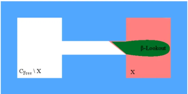
First, the β–lookout, Definition 2.2.4 and Figure 2.3, of a subset X of Cf ree is the portion of X that can see at least aβ fraction of the compliment of X. In this way, β relates to the probability of sampling a new configuration that can expand the visibility of X.

Definition 2.2.4. Let β be a constant in (0,1]. The β–lookout(X) [41] of a set X ⊆ Cf ree is the set of configurations of X which can connect to at least aβ fraction

(34)

Figure 2.3: Set X (red) and its β–lookout (green).

of the compliment of X, that is

β–lookout(X) = {q∈X|µ(V(q)\X)≥βµ(Cf ree\X)}.

With this definition in hand, the full definition of (ǫ,α,β)–expansiveness is given in Definition 2.2.5.

Definition 2.2.5. Let ǫ, α, β be constants in (0,1]. A configuration space Cf ree is

(ǫ, α, β)–expansive [41] if 1. Cf ree is ǫ–good

2. For any set M of points, the β–lookout(V(M)) is at least an α fraction of the hypervolume of V(M), that is

µ(β–lookout(V(M)))≥αµ(V(M)).

A higher α and β describe an easier ability to expand and connect a roadmap of Cf ree through sampling-based planning. (ǫ, α, β)–expansiveness is an inherent property of Cf ree for a given motion planning problem which cannot be altered. Additionally, these parameters are as difficult to compute explicitly as computing

(35)

∂Cobst. Despite this, the parameters can help understand trends in the expected number of samples and how the probability of finding a solution corresponds to the difficulty of the space. Specifically, with probability at least 1−γ, a roadmap of

n =⌈16 ln(8/ǫαγ)/ǫα+6/β+4⌉nodes chosen uniformly at random will be connected, where γ ∈(0,1) [42].

2.2.5 Workspace-biased Planning Methods

Many planners use workspace information, e.g., regions or decompositions, to aid in the planning process. Here we describe a few relevant frameworks.

Feature Sensitive Motion Planning [73, 75] recursively subdivides the space into “homogeneous” regions (regions of the environment containing similar properties, e.g., free or clutter), individually constructs a roadmap in each region, and merges them together to solve the aggregate motion problem. This framework adaptively determines the specific planning mechanism to map to each homogeneous region, e.g., choosing OBPRM in cluttered regions and uniform sampling in open regions. Similar frameworks have been proposed [85, 97]. RESAMPL samples spherical re-gions in the space and uses entropy information to decide on the specific planner to use [85]. The Unsupervised Adaptive Strategy (UAS) uses a K-means clustering algorithm to learn important regions of the space and then applies Hybrid PRM in each region [97]. Hybrid PRM uses a reward-based learning mechanism to adaptively select appropriate sampling schemes for a space [44]. A recent approach, Adaptive Neighborhood Connection (ANC), extends Hybrid PRM to connection [30]. ANC could also be incorporated into UAS, but this direction has yet to be explored.

Other approaches utilize workspace decompositions to find narrow or difficult ar-eas of the workspace to bias Cspace sampling [98, 57, 79]. These methods begin by decomposing the workspace using an adaptive cell decomposition [98] or a

(36)

tetrahe-dralization [57], and then weight the decomposition to bias sampling. However, by automatically identifying regions and disallowing dynamic region specification and modification, the planner might suffer from inefficiencies, such as oversampling in a fully covered region. Additionally, these planners do not typically consider regions that repel sampling.

Some approaches deviate from standard sampling-based methodologies and use heuristic guided search mechanisms built from the A∗ _{methodology. One such} ap-proach uses an A∗_{-like approach to find a workspace path of overlapping circles, and} then uses this to heuristically search for a path composed of predefined kinematic motions [14]. This has been extended to modeling traffic scenarios [15] and dynamic environments [16]. This method however has difficulty extending past 2-dimensional workspaces, car-like robots, and simplistic obstacles.

2.3 User-guided Motion Planning

In many approaches to human-assisted planning, a human operator (user) per-forms global analysis of the workspace to determine an approximate solution while the machine handles high-precision tasks such as collision detection. In [45, 8, 99] the user can select configurations that are critical to finding a collision-free path, while the planner performs collision checking and path-finding between sub-goals (shown as Cfg Input in Figure 2.4). Certain approaches allow a user to input an approximate path in the scene, and an autonomous planner then morphs this motion into a fea-sible plan [8, 59, 102] (shown as Path in Figure 2.4). Often, these types of planners have distinct phases for user input and automated planning.

More recently, a two-way communication approach was developed for RRTs, called Interactive-RRT (I-RRT) [94]. In this system, the planner and the user inter-act in an online fashion to cooperatively solve the problem. I-RRT allows the user

(37)

Interface Complexity (DOFs)

Expected User Involvement

Autonomous Manual c w SBMP I-RRT Region Steering Cfg Input

Path_{Teleoperation}Bilateral

LfD-PbD

Cspace

Crowd-Sourcing

Figure 2.4: Interface complexity in terms of degrees of freedom manipulated versus level of autonomy in expected behavior, where c is the degrees of freedom of the Cspace and w is the degrees of freedom of the workspace is shown. The approach described in Chapter 4, called Region Steering here (underlined), is a combination of high autonomy mixed with a simple interface.

to control a robot avatar that biases RRT growth in a virtual scene. This approach, however, is limited to single-query scenarios, requires continuous user input, and is constrained to robotic systems that are fully controllable by the avatar interface (as seen in Figure 2.4).

2.3.1 Crowd-sourcing

There is a distinct but related approach to user-guided planning by which crowd-sourcing is used to steer a large swarm [10] or perform protein folding [9]. In these solutions, a single problem is given to a large number of people in the hopes of finding a global solution or deriving a future control law. However, these approaches have a separate goal compared with user-guided planning, in that user-guided planning allows a user to interact directly with the planner. Despite the different goals how-ever, these approaches can inform each other on best practices in interfacing with a user.

(38)

2.3.2 Bilateral Teleoperation

Teleoperation approaches provide closed-loop interactions between an operator and a robot such that the operator has a sense of presence-at-a-distance [38]. Tele-operation focuses on capturing and/or augmenting a user’s mechanical skills directly. Often, these approaches try to assist the human operator by predicting where the user is headed, ensuring proper collision avoidance, and maximizing user control over the system [63]. However, these approaches provide minimal automation focusing on presence-at-a-distance allowing human operators to perform tasks in typically dangerous environments, e.g., exploration in space, oceans, or volcanoes. In con-trast, human-in-the-loop planning aims to leverage a user’s high-level intuition by augmenting an automated planner with information about difficult aspects of the problem.

Nonetheless, both seek to provide a form of two-way communication, referred to as bilateral control in teleoperation literature. Often these approaches have a high interface complexity, e.g., using haptic devices with many degrees of freedom and provide as much control to the user as possible (Figure 2.4). A recent study in teleoperation [69] shows that this form of interaction can be burdensome on the user, e.g., in situations with cyclic or repetitive motions, and takes steps to provide the robot with greater autonomy so that the user need only provide global guidance rather than direct control. Other teleoperation systems allow the user to control a subset of the robot’s dofs through a precomputed Cspace, as in [48, 47], but these are limited to low dimensional problems. This approach is referred to as Cspace in Figure 2.4.

(39)

2.3.3 Robot Learning from Demonstration

In Robot Learning from Demonstration (LfD) or Robot Programming by Demon-stration (PbD), a human operator trains a robot to perform a new task that the robot has never done before [6]. Typically, this involves a user physically moving the robot through the task. Afterwards, the robot extracts features of this task, i.e., important aspects of the motion or task, and attempts to extrapolate a new control law to com-plete the task. LfD-PbD research is multi-faceted towards solving various questions such as what tasks should/can be imitated, how to compute/perform an imitation, when can a robot imitate, and whom should the robot imitate [20]? A good example of LfD-PbD is in preparing food using a robot, e.g., pouring ingredients or flipping a pancake [54].

LfD-PbD is in some ways the opposite of teleoperation. In teleoperation, a robot is used to augment a human in various ways, e.g., being physically present on another planet when the human cannot. However, in LfD-PbD a human augments a robots task capabilities by teaching a robot something the human already knows how to do. Naturally, user-guided motion planning is similar to both. In the case of LfD-PbD, a human manually performs the task for the robot upon which a robot then learns and extrapolates information of the task. However, in user-guided planning a higher level of collaboration is sought. There, the human attempts to cooperatively complete a task, e.g., motion planning, splitting the work with the automated abilities of the robot, i.e., the human does high level thinking while the robot does low level computations. Again, we believe that these fields can learn from each other, in the same way user-guided planning might learn from teleoperation and/or crowd-sourcing applications.

(40)

3. USER-GUIDED PLANNING

In this chapter, we classify and model common user-guided approaches discussing the interface requirements and trade-offs in the context of sampling-based planning. We augment our discussion with experimental analysis.

3.1 Models of User-guidance

User-guided planners encompass methodologies to limit the search space of the planner through user input. By specifying a presumably important (or unimportant) portion ofCspace, the user restricts the planner to focus on a particular subset ofCspace. For example, if a region biases PRM construction, e.g., to a narrow passage, then the planner will focus and build a denser roadmap in the narrow passage as compared with the portions of theCspacenot covered by the region. Thus, collaborative planners have the potential to provide more effective planning.

There are a few important design considerations when implementing a collabo-rative motion planner. First, rendering and feedback should be real-time, or close to real-time, to allow a seamless collaboration. Second, an intuitive mechanism for region specification is needed. Finally, proper user feedback should be customized for the planner. For example, a region might be colored based upon an algorithm-specific perception of usefulness.

Additionally, there is an important trade-off to be made based on PRM time versus the time taken for the user. Essentially, user-guidance can only truly help if the time taken between capturing the user input and planning with it is less than an unaided planner. Our recent work, which is also the core subject of this dissertation (Chapter 4), has shown this is viable for region-based input [27, 26].

(41)

and modeling of user-guided methods into three categories based upon their input modalities: configuration-based input, path-based input, and region-based input.

3.1.1 Configuration-based Input

First, we define a basic model of input where a user places specific configurations in Cf ree to act as waypoints for a sampling-based motion planner, e.g., [45]. We call these augmenting configurations “beacons.” To specify a configuration the interface must have an equal number of degrees of freedom as the robot itself. Hence, it might be prohibitive or expensive to design such an interface which is intuitive and easy to use — we note you could have a user simply specify all dofs explicitely, but this might not be intuitive.

Because of the precision required and interface complexity related to gathering this information, this methodology of user-guidance may not be ideal in terms of total planning time. However, this input modality will aid in solving a motion planning problem when a user specifies a difficult configuration. In this way, it would provide a divide-and-conquer approach to planning, where the planner solves the problem from the start to each beacon in order and then to the goal.

3.1.2 Path-based Input

In the path-based input model, the user provides a set of paths Π (Definition 2.1.8) in Cf ree. A few methods do allow for path specification approximately [8, 59, 102], and then modify the path to be in Cf ree. However, the input device would require full control of a robot, and might be prohibitive to design a simple and intuitive interface for all robot types.

Here we specifically study a simplified model for our motion planners in which we assume that the end points of each path are added as nodes to the roadmap, and the path is then added as an edge in the same graph. After, a planner progresses as

(42)

normal.

3.1.3 Region-based Input

Some approaches allow the user to specify approximateCspaceregions, e.g., [94, 27, 26]. The regions are then used to bias the sampling phase of a sampling-based planner to steer planning toward or away from specific portions of Cspace. An interesting aspect of this type of input is that in order to specify a region of Cspace a user does not specifically require an interface with numerous of degrees of freedom. Rather, a low dimensional device can be used (see [27, 26]) — this makes designing interfaces and algorithms with this input modality especially attractive.

Region-based input can be approximate in its specification and still encapsulate knowledge of the difficult portions of the planning space. In problems where the workspace shows strong correlation with the Cspace narrow passages, then region-based input is particularly useful. For example, a user can place a region around the workspace narrow passage to effectively guide the planner through the narrow passage.

3.2 Experimental Analysis of User Input Modalities

In this experiment, we study the impact of user-guided planning on PRMs by comparing a PRM’s performance with and without the various types of user inputs. Specifically, we explore the effect of the three user models: configuration-based input (Cfg), path-based input (Path), and region-based input (Region). We show that the various user inputs can all aid a sampling-based planner in discovering a solution more efficiently than the planner alone, and we highlight differences in each input’s effectiveness. Specifically, we show that, while path-based input might help solve the problem the fastest compared with both configuration-based and region-based input, region-based input allows for a nice trade-off of ease of input and planner efficiency.

(43)

3.2.1 Setup

All methods were implemented in a C++ motion planning library developed in the Parasol Lab at Texas A&M University. It uses a distributed graph data structure from the Standard Template Adaptive Parallel Library (STAPL) [12], a C++ library designed for parallel computing.

All experiments were run on a Dell Optiplex 9010 running Fedora 20 with an Intel(R) Core(TM) i7-3770 CPU with 24 GB of RAM with the GNU gcc compiler version 4.8.3.

All methods use uniform random sampling, Euclidean distance, straight-line local planning, and a k = 10-closest connection strategy. In all cases of input, high school students provided the key configurations, paths, or regions to satisfy the assumptions of the corresponding models. For configuration-based input, configurations were placed approximately as knowing the exact placements of configurations might not be obvious in a given problem instance. The same input is used for each trial of our experiments. Trials are run until either 10,000 nodes are sampled or a representative query is solved for a scenario.

We compare these different methods in a variety of toy scenarios featuring various types of narrow passages:

• STunnel (Figure 3.1(a)) – A simple 2 dof square robot traverses a difficult S-like narrow passage from top to bottom.

• ZTunnel (Figure 3.1(b)) – A 6 dof cube robot must pass through a difficult Z-shaped narrow passage between the ends of the environment.

• MazeTunnel (Figure 3.1(c)) – A 6 dof spinning-top meanders through a com-plex series of tubes from top to bottom.

(44)

Table 3.1: Success rates of experimental methods.

STunnel ZTunnel MazeTunnel Walls Hook

PRM 40% 80% 100% 0% 60%

Cfg 100% 100% 100% 100% 90%

Region 100% 100% 100% 100% 100%

Path 100% 100% 100% 100% 100%

• Walls (Figure 3.1(d)) – A 7 dof articulated linkage must cross a series of narrow passages (walls with holes) from one end of the environment to the other.

• Hook(Figure 3.1(e)) – A 10doffree-flying articulated linkage bridges two ends of the environment through a narrow slit in a central wall.

For each trial, we recorded the number of nodes in the final roadmap, the number of collision detection (CD) calls for construction, the time it takes to build, and whether the planner succeeded or not in solving the query in under 10,000 nodes.

3.2.2 Results

We performed ten trials and reported averages of all runs, successful or not, i.e., we average failed cases (as a best case metric for that specific trial) as well. Success rates are shown in Table 3.1 and metrics are shown in Figure 3.2. We also note that we are not including computations needed for capturing the input, and discuss this trade-off in the discussion below.

Figure 3.2(a) shows the average number of nodes it took to construct a roadmap to solve the example query. As we can see by this plot, all of the user-based methods solved the scenario with fewer nodes than standard PRM. Figure 3.2(b) shows the average number of CD calls, and Figure 3.2(c) exhibits the average time in seconds each method took to solve the problem. These metrics further indicate that using

(45)

(a) STunnel(2 dof) (b) ZTunnel(6dof)

(c) MazeTunnel(6dof)

(d) Walls(7 dof) (e) Hook(10dof)

Figure 3.1: Test scenarios. The start (solid red) to end (hollow blue) of an example solution path is shown.

(46)

1 10 100 1000 10000

Nodes PRM Cfg Path Region (a) Nodes 1 10 100 1000 10000 100000

CD Calls PRM Cfg Path Region (b) CD Calls 0.001 0.01 0.1 1 10 100 1000

Time(s) PRM Cfg Path Region (c) Time

Figure 3.2: Experimental results for building a roadmap without user-input (PRM), configuration-based input (Cfg), path-based input (Path), and region-based input (Region). (a) Number of nodes, (b) number of CD Calls, and (c) time in seconds to solve the representative query averaged over ten trials are shown.

user input solves our example problems faster than PRM alone.

An interesting aspect of the data which we discuss more below is that Path generally outperformed Region which in turn outperformed Cfg. The only case this did not hold is in ZTunnel. In this case, the specific placements of configurations used avoided the rotational challenge of the narrow passage. They were placed at each turn and reduced the difficulty of the passage to just a translational problem. However, this was not possible with the regions. Moreover, this is a specific narrow

(47)

passage and this effect is unlikely to happen in practice. 3.3 Discussion

User-guided planing has been shown to improve over PRM in each of our toy environments. User-guidance helps PRM through the narrow passage by aiding the planner specifically with the most difficult aspects of the problem. That is to say for example with Cfg, the input configurations give PRM waypoints representing the most difficult aspects of the problem. In other words, the area PRM has to search for a solution is reduced by adding critical information from the user. Cfg, Region, and Path all perform well and show that these forms of user input are viable tools to aide future planners.

Figure 3.2 displays an interesting trend that Path required fewer nodes than Region, which requires fewer nodes than Cfg. The main intuition behind this trend is as follows. First, Path input clearly avoids PRM’s need to map any configurations in the most difficult portions of a problem. In other words, Path acts as another planner giving a partial solution path to the overall problem reducing the work the PRM has to do. Second, both Cfg and Region still require sampling and connection phases of PRM to finish solving the problem. With Cfg, the need to sample critical configurations is avoided and requires only connection. With Region, a method will still need to sample and connect in difficult portions, but the probability of doing so is altered based on the placement of regions. Finally, Region generally can beat Cfg because it, again, alters the underlying sampling process biasing it towards difficult portions of the space.

(48)

4. REGION-BASED COLLABORATIVE PLANNING∗

In this Chapter, we describe our general framework for region-based collaborative planning, through which an automated planner and a human operator, referred to as a user, interact to cooperatively discover a solution to a motion planning problem. The general idea is that a user specifies regions of the workspace to bias a planner in Cspace, and the planner informs the user of its progress by displaying the current roadmap and possibly some indications of region usefulness.

4.1 Framework

Our framework provides a methodology to limit the search space of the planner. By specifying a presumably important (or unimportant) workspace region R, the user restricts the planner to focus on a particular subset of Cspace. For example, if a region biases PRM construction, e.g., to a narrow passage, then the planner will focus and build a more dense roadmap in the narrow passage as compared with the portions of theCspace not covered by the region. Thus, our collaborative planner has the potential to provide more effective and efficient planning in terms of coverage and plan construction time.

To provide an intuitive mechanism for region specification, we allow a user to specify either Axis-Aligned Bounding Box (AABB) or Bounding Sphere (BS) regions for their simplicity and the ability to specify them with a common mouse interface. Note, we do not claim that the user interface is optimal or intuitive: it is merely sufficient for the user to communicate with the planner and allows us to study the ∗_{The description of the method and some of the experimental results are reprinted from}

Algo-rithmic Foundations of Robotics XI, “A Region-based Strategy for Collaborative Roadmap Con-struction,” volume 107, 2015, pp. 125–141, J. Denny, R. Sandstr¨om, N. Julian, and N. M. Amato,

c

(49)

Figure 4.1: Alpha puzzle. A pathologically difficult motion planning problem in which the two α shaped peices must be separated.

usefulness of our collaboration framework. We leave further development of the interface to future work.

While our framework is quite general, it is important to note that our workspace regions are primarily effective in problems where the translational degrees of freedom dominate the system. This occurs often in systems such as mobile robots, unmanned aerial vehicles, or certain CAD applications. In contrast, applying this framework in other scenarios such as strongly rotational problems (e.g., the alpha puzzle, shown in Figure 4.1) would require an alternative region type to successfully limit the planner.

4.1.1 Overview

Our two-way communication framework is shown in Figure 4.2.

In one direction, the user specifies workspace regions to bias the planner. Regions have “types,” that can be arbitrarily extended for a particular application. By default, we allow two kinds of regions: attract (bias the planner) and avoid (disallow plans in this region). We allow these regions to be modified at any time, including addition of new regions, resizing/repositioning of current regions, and deletion of regions from the planning scene.

(50)

Figure 4.2: In one direction, the user specifies workspace regions, and in the other direction, the planner displays the current progress in planning.

For sampling-based planners this would be the current roadmap being constructed, whether it is a graph or a tree. The tree is drawn by embedding the d-dimensional tree in the 2- or 3- dimensional workspace. Nodes are drawn by a point located at its positional data. Nodes in the same connected component are displayed with the same color so that the user can easily determine whether two nodes are connected. Edges are displayed as polygonal chains of intermittent configurations along the edge. Additionally, we present the current regions to the user. Our framework is able to present a perceived usefulness of regions and recommend regions to the user.

The algorithmic framework for the automated planner shown in Algorithm 3 fol-lows this scheme. Generally, it performs a loop until the planner is finished, e.g., solves an example query or reaches a specific number of nodes. In each iteration, a specific planner biased by the user-defined regions first does automated planning.

(51)

Algorithm 3 Region-based Collaborative Motion Planning Framework Input: Environment e Output: Roadmap G 1: G= (V, E)←(∅,∅) 2: while ¬done do 3: r←SelectRegion(e.regions) 4: RegionBiasedPlanner(G, e, r) 5: G.UpdateMap() 6: e.UpdateRegions() 7: return G

Next, the planner provides feedback to the user through the roadmap and region displays. This is important visual information to help the user adjust regions appro-priately.

4.1.1.1 Example

Figure 4.3 shows a simple example that illustrates the general progression of our algorithm in a 2D envir