Journal of Information Sciences and Computing Technologies(JISCT) ISSN: 2394-9066
SCITECH
Volume 4, Issue 3
RESEARCH ORGANISATION|
October 10, 2015
Journal of Information Sciences and Computing Technologies
www.scitecresearch.com/journals
Modeling and Optimizing of a Non-constrained
Multi-Objective Problem having Multiple Utility Functions Using
the Bayesian Theory
Pooneh Abbasian
1, Nezam Mahdavi-Amiri
2, Hamed Fazlollahtabar
31Department of Industrial Engineering, Mazandaran University of Science and Technology, Babol, Iran. 2Faculty of Mathematical Sciences, Sharif University of Technology, Tehran, Iran
3Faculty of Management and Technology, Mazandaran University of Science and Technology, Babol, Iran.
Corresponding author's email: [email protected]
Abstract
One of the multi-objective optimization methods makes use of the utility function for the objective functions. A utility function induces the most satisfactory solution for a decision maker (DM) by considering DM’s priorities. In existing studies, there are only one utility function for each objective function. But due to practical situations in different decision making environments in an industry or a trade, each goal may have multiple utility functions. Here, we present a multi- objective model in which each objective function has multiple utility functions applying Bayesian theory. The model allows the DM to calculate the probability of the utilities using conditional probability in conditions of certainty. Examples are worked through to illustrate the usefulness of the proposed model.
Keywords
:
Utility function; Multiple-objective decision making; Goal programming; Multi-choice goal programming; Bayesian theory.1.
Introduction
Multi-objective optimization (also known as multi-objective programming, vector optimization, multi criteria optimization, multi attribute optimization or Pareto optimization) is concerned with multiple criteria decision making, which entails mathematical optimization problems involving more than one objective function to be optimized simultaneously.The goal may be to find a representative set of Pareto optimal solutions, and/or quantify the trade-offs in satisfying different objectives, and/or finding a single solution that satisfies subjective preferences of a human decision maker (DM). As shown by Romero et al. [1], multi-objective programming (MOP) models particularly goal programming (GP) ones, can be considered as special cases of the distance function model (DFM).
A classical DFM can be expressed as follows:
(
DFM
) :
1 * 1 [ | (x) |] , . . , n p p j j j j Min w f f s t x F
Journal of Information Sciences and Computing Technologies(JISCT) ISSN: 2394-9066 where the wi, fi*, and fi(x) are respectively the weight factors, aspiration levels (goals), and achievement functions of theith goal, for i= 1,...,n and | * ( ) |
i i
f f x is the absolute deviation between the achievement function of
theith goal and its aspiration level [29].
A goal program is an important model for helping DMs to solve multi-objective decision making (MODM) problems. GP has been one of the most commonly used methods in solving multiple objective/criteria decision making (MODM/MCDM) problems since Charnes et al. [2] introduced the concept of GP. Mathematical aspects of GP was first introduced by Charnes and Cooper [3], and further developed by Lee [4], Ignizio[5], Tamiz et al. [6] and Romero [7], among others (see [8-10]). The purpose of GP is to minimize the absolute deviations from specified purposes. The approach considers some predetermined goals. Because of resource limitations, DMs aim to minimize the deviations of the achievement functions from the goals [8].
A GP formulation can be shown as follows:
| | 1 a feasible set : n Min f (x) - gi i i = X F (F, , G ) Ps.t.
where the f xi( ) are the achievement functions and the gi are the aspiration levels.
There are various types of methods being used to solve a GP problem. Some examples are: Lexicographic GP (LGP), Weighted GP (WGP), and Min-Max (Chebyshev) GP (see [7, 11]). A WGP formulation is as follows:
( ) 1 , 0 : , 1,..., , , 1
n Min i id i id i + -s.t. f (x) - di i + di = g ,i di d i n W GP i = ,… i , x , F nwhere di+ and di- are over and under achievement of the ith objective function (goal), respectively, αi and βi are the weights attached to these deviations, respectively, fi( )x and
g i
are defined as in GP [8]. Tamiz et al. [12] showed that about 64% of GP applications involve LGP and 21% consider WGP in the literature. There are other types of GP, namely the MIN-MAX program introduced by Flavell [13] in which the maximum deviation is to be minimized. This has a close relation to fuzzy goal programming (FGP) introduced by Zimmerman [14]. In GP methods a normalization process to overcome the incommensurability is used. When we roll up some of the deviation variables that have different units of measurement, incommensurability occurs. Here, we consider normalization process (1) Percentage normalization [15], (2) Euclidean normalization [16, 17], (3) Summation normalization [18], (4) and Zero-one normalization [19]. At timesDM’s note that the actual result of operation is greater than the aspiration level defined. In other words, they could define more aspiration levels under the available resources. This event is called underestimation problem. multi-criteria method was presented by Wierzbicki[20] to search around the aspiration levels to avoid the underestimation problem. In this case, a new method was presented to solve the problem in which DM’s set more aspiration levels in the initial stage of the process by the use of multi-choice aspiration levels (MCAL) [8]. The important point is that all the GP approaches only solve problems each of which has one aspiration level on the right hand side of the equation, whereas in real world, more aspiration levels may be considered [28]. The above mentioned problem cannot be solved by GP approaches, since Chang proposed the multi-choice goal programming (MCGP) [8; 9]. The achievement function of MCGP can be expressed as follows: 1 1 1 1 1 a feasible set n + -Min w (di i + d )i i = m + -s.t. f (X ) - di i + di = gijSij(B), j = i = ,..., n, + -di ,di 0, i = ,..., n, Sij(B) R (x),i j = ,..., m X F (F, ), Journal of Information Sciences and Computing Technologies(JISCT) ISSN: 2394-9066 where Sij(B)is the jth function of binary serial number, Ri(x) represent the function of resource limitations, and the other variables are as defined in WGP. Following the idea of MCGP, Liao [21] presented multi-segment goal programming (MSGP), where the existence of multiple coefficients for the decision variables was possible.
A utility function (UF) is the most widely used tool in presenting a DM’s priorities investigated by Al-Nowaihi et al. [22], Yu et al. [23], and Podinovski [24]. Following the idea of Chang [25], here we use probability of the utility function as an aspiration level of GP or MCGP. There are only four possible shapes for the utility functions: convex, concave, S-shaped and reverse S-shaped. Here, we use linear utility functions [25]. Our aim is to optimize the multiple-objectives without restriction model with, each objective having multiple utility functions. In the literature, no work has been done on how to solve the multiple-objectives problem with multiple utility functions. The issue in MODM problems is to investigate different conditions arising from the utilities of each objective. We solve this problem by calculating the probability of each utility function.
The rest of our work is organized as follows. In Section 2, problem description associated with the optimization model are presented. To show the effectiveness of the proposed model, an example is illustrated in Section 3. Finally, conclusions are given in Section 4.
2. Modeling and optimizing un-constrained multi-objective problem
In real-life situations, in different decision making environments in industry or trade, different utilities need to be considered for each objective .This is due to the impact of environmental factors in the optimal solution. In the literature, available models consider only one utility function for each objective. To consider multiple utilities, here we propose a model to calculate the probability of each utility function. Our goal is to calculate the probabilities using Bayesian theory [26]. Bayesian probability theory caters a mathematical framework for inference and reasoning using possibilities. Bayesian probability theory was laid down by Bernoulli, Bayes, and Laplace (see [26]). Our approach makes use of the Bayes' rule as follows.
Bayes' rule
:
If B1,…,Bk partition a space S, and A is an ideal event, then.
where P(Br | A)denotes the conditional probability for the occurrence of event Br, given that the event A has already occurred [26]. A multi-objective without restrictions model can be expressed as follows:
1 ( Max Min) ( ) { ( ),..., ( )} ( , a feasible set). n or F X f x f x s.t. X F F
Here, we consider utilities 1
i i, pi
u ,...,u
for each objective function fi. Assuming that the utilities1
11 1,p
u ,...,u
corresponding to the first objective are incompatible with each other, we can calculate the probability of the utilities using Bayesian theory as follows:1 1 1 1 1 1 1 1 1 ( ) ( | ) ( ) ( | ) , , 1,..., , 1,..., . (1) ( ) ( | ) ( ) r i i r r r i p i i j j j p u x p x u p u p u x i i n r p p x p x u p u
We can expand Eq. (1) :
1 ( ) ( | ) ( ) ( | ) , , , , 1,..., , 1,..., , 1,..., . (2) ( ) ( | ) ( )
i i r j j i r i r i r j p i j j ik ik k p u x p x u p u p u x i j r i n j m r p p x p x u p u | P(Br A) P(B )* P(A | B )r r 1 P(Br A) = = , i = ,..., k, P(A) iP(B )* P(A | B )i i Journal of Information Sciences and Computing Technologies(JISCT) ISSN: 2394-9066 Regarding the definition of prior and posterior probabilities, DM can set prior probabilities for the utility functions in order to access the conditional probabilities above. This new conditional probability of uir is called posterior probability. This way, we can use the total probability rule for the objective function fi to reach final probabilities, as shown below: 1 ( ) ( | ) ( ) , , , 1,..., , 1,..., . (3) m ir ir j j i j p u p u x p x i r i n r p
Now for each fi, let p u( i1),...,p u( i, pi)
be the aspiration levels achieved.
We use the definition of the sum of the probabilities to combine all the final probabilities (Eq. (3)) for each objective separately. Now, each objective has only one probability value. Taking the probability value as an aspiration level of the objective function, we know that the problem with only one aspiration level can be solved using the GP formulation. The purpose of GP is to minimize the deviations between achievement of goals and their aspiration levels. This problem can be solved by WGP and can be expressed as the following program:
1 Min [ ( )] ( ) , 1,..., , , , 0, , n i i i i i i i i i i w d d s.t. f x d d g i n d d x x F
where
g
i
is sum of probabilities of the utility functions corresponding to the ith goal.If we do not use the definition of the sum of probabilities, then we have multiple probability value for each objective function. Consider the values as aspiration levels of the objective function. To the best of our knowledge, the problem with multiple aspirations cannot be solved by current GP approaches .This problem can be solved by an MCGP approach and can be expressed as follows:
1 1 1 1 1 a feasible set n + -Min wi(di + di ) i = m + -s.t. fi(X ) - di + di = gijSij(B), j = i = ,..., n, -di ,di 0, i = ,..., n, Sij(B) R (x),i j = ,..., n, X F (F, ),
where
g
ij is the jth aspiration level corresponding to the ith goal.3. Illustrative example
Consider a problem with the corresponding goal and utility functions; we assume two cases of independence and dependence of variables:
1 1 2 3
Goal 1: max f ( )x 3x 2x x . Utility functions corresponding to
1 f : 11 1 2 3 12 1 2 13 1 2 3 ( ) 2 3 2 ( ) 2 ( ) . u x x x x u x x x u x x x x
Journal of Information Sciences and Computing Technologies(JISCT) ISSN: 2394-9066 The inputs: p u( 11)0.25, p u( 12)0.5, p u( 13)0.25, 1 11 2 11 3 11 1 12 2 12 1 13 2 13 3 13 ( | ) 0.35 ( | ) 0.3 ( | ) 0.35 ( | ) 0.5 ( | ) 0.5 ( | ) 0.23 ( | ) 0.74 ( | ) 0.03. p x u p x u p x u p x u p x u p x u p x u p x u
If x1, x2 and x3 are assumed to independently affect the utility functions, then we arrive at the following probabilities: 1 1 11 11 1 12 12 1 13 13 2 2 11 11 2 12 12 2 13 13 3 ( ) ( | ) ( ) ( | ) ( ) ( | ) ( ) (0.35)(0.25) (0.5)(0.5) (0.23)(0.25) 0.39 0.4 ( ) ( | ) ( ) ( | ) ( ) ( | ) ( ) (0.3)(0.25) (0.5)(0.5) (0.74)(0.25) 0.51 ( ) p x p x u p u p x u p u p x u p u p x p x u p u p x u p u p x u p u p x p ( 3| 11) ( 11) ( 3| 13) ( 13) (0.35)(0.25) (0.03)(0.25) 0.09 x u p u p x u p u 1 11 11 11 1 1 2 11 11 11 2 2 3 11 11 11 3 3 ( | ) ( ) (0.35)(0.25) ( | ) 0.22 ( ) 0.4 ( | ) ( ) (0.3)(0.25) ( | ) 0.15 ( ) 0.51 ( | ) ( ) (0.35)(0.25) ( | ) 0.97. ( ) 0.09 p x u p u p u x p x p x u p u p u x p x p x u p u p u x p x
By using the total probability rule, we obtain:
11 11 1 1 11 2 2 11 3 3 ( ) ( | ) ( ) ( | ) ( ) ( | ) ( ), p u p u x p x p u x p x p u x p x 11 ( ) (0.22)(0.4) (0.15)(0.51) (0.97)(0.09) 0.25. p u
On the other hand, if x1,x2,x3 dependently affect the utility functions, then with the following data,
we get the following probabilities:
2 1 3 1 3 2 2 11 1 3 1 11 3 2 11 3 11 1 2 3 1 2 ( | ) 0.1 ( | ) 0.75 ( | ) 0.35 ( | ) 0.1 ( | ) 0.5 ( | ) 0.45 ( | ) 0.15 ( | ) 0.64, p x x p x x p x x p x u x p x x u p x x u p x u x x p x x x
Journal of Information Sciences and Computing Technologies(JISCT) ISSN: 2394-9066 1 11 11 2 11 1 11 1 2 1 2 1 1 11 11 3 1 11 11 1 3 1 3 1 2 11 11 3 11 2 3 ( | ) ( ) ( | ) (0.35)(0.25)(0.1) ( | ) 0.22 ( ) ( | ) (0.4)(0.1) ( | ) ( ) ( | ) (0.35)(0.25)(0.5) ( | ) 0.15 ( ) ( | ) (0.4)(0.75) ( | ) ( ) ( ( | ) p x u p u p x u x p u x x p x p x x p x u p u p x x u p u x x p x p x x p x u p u p x p u x x 2 11 2 3 2 3 11 1 2 2 11 1 1 11 11 11 1 2 3 3 1 2 2 1 1 | ) (0.3)(0.25)(0.45) 0.19 ( ) ( | ) (0.51)(0.35) ( | ) ( | ) ( | ) ( ) ( | ) ( | ) ( | ) ( ) (0.15)(0.1)(0.35)(0.25) 0.05. (0.64)(0.1)(0.4) x u p x p x x p x u x x p x u x p x u p u p u x x x p x x x p x x p x 1 2 2 1 1 1 3 3 1 1 2 3 3 2 2 1 2 3 3 1 2 1 2 ( ) ( | ) ( ) (0.1)(0.4) 0.04 ( ) ( | ) ( ) (0.75)(0.4) 0.3 ( ) ( | ) ( ) (0.35)(0.51) 0.18 ( ) ( | ) ( ) (0.64)(0.04) 0.03. p x x p x x p x p x x p x x p x p x x p x x p x p x x x p x x x p x x
By using the total probability rule, we obtain:
11 11 1 2 1 2 11 1 3 1 3 11 2 3 2 3 11 1 2 3 1 2 3 11 ( ) ( | ) ( ) ( | ) ( ) ( | ) ( ) ( | ) ( ) ( ) (0.22)(0.04) (0.15)(0.3) (0.19)(0.18) (0.05)(0.03) 0.09. p u p u x x p x x p u x x p x x p u x x p x x p u x x x p x x x p u
The same calculations can be carried out for the other two utility functions. Using the given inputs below:
2 12 1 2 1 13 3 1 13 3 2 13 3 13 1 2 3 1 2 ( | ) 0.1 ( | ) 0.3 ( | ) 0.35 ( | ) 0.21 ( | ) 0.73 ( | ) 0.64, p x u x p x x u p x x u p x x u p x u x x p x x x we get 12 12 1 1 12 2 2 ( ) ( | ) ( ) ( | ) ( ) (0.62)(0.4) (0.5)(0.51) 0.5 . p u p u x p x p u x p x 1 12 12 2 12 1 12 1 2 1 2 1 ( | ) ( ) ( | ) (0.5)(0.5)(0.1) ( | ) 0.62. ( ) ( | ) (0.4)(0.1) p x u p u p x u x p u x x p x p x x 12 12 1 2 1 2 ( ) ( | ) ( ) (0.62)(0.04) 0.02. p u p u x x p x x 13 13 1 1 13 2 2 13 3 3 ( ) ( | ) ( ) ( | ) ( ) ( | ) ( ) (0.14)(0.4) (0.36)(0.51) (0.08)(0.09) 0.25. p u p u x p x p u x p x p u x p x 13 13 1 2 1 2 13 1 3 1 3 13 2 3 2 3 13 1 2 3 1 2 3 ( ) ( | ) ( ) ( | ) ( ) ( | ) ( ) ( | ) ( ) (0.43)(0.04) (0.07)(0.3) (0.22)(0.18) (0.49)(0.03) 0.09. p u p u x x p x x p u x x p x x p u x x p x x p u x x x p x x x
For the sake of simplicity, but without the loss of generality, we considered two other goals with utility functions as follows: 2 2 3 3 1 2 3 Goal 2 : Max ( ) 3 2 , Goal 3 : Max ( ) 3.5 5 3 . f x x x f x x x x
Utility functions of f2 and f3 are:
21 2 3 22 2 3 31 1 3 32 1 2 3 2 2 2 3 5 3 , u x x u x x u x x u x x x
Journal of Information Sciences and Computing Technologies(JISCT) ISSN: 2394-9066 with the following data:
21 22 31 32 ( ) 0.45 ( ) 0.55 ( ) 0.38 ( ) 0.62. p u p u p u p u
Doing similar computations as before, we arrive at the final probabilities as specified below:
21 21 2 2 21 3 3 ( ) ( | ) ( ) ( | ) ( ) (0.23)(0.33) (0.08)(0.12) 0.09, p u p u x p x p u x p x 2 21 21 3 21 2 21 2 3 2 3 2 ( | ) ( ) ( | ) (0.17)(0.45)(0.29) ( | ) 0.17, ( ) ( | ) (0.33)(0.4) p x u p u p x u x p u x x p x p x x 21 21 2 3 2 3 ( ) ( | ) ( ) (0.17)(0.13) 0.02, p u p u x x p x x 22 22 2 2 22 3 3 ( ) ( | ) ( ) ( | ) ( ) (0.78)(0.33) (0.92)(0.12) 0.37, p u p u x p x p u x p x 2 22 22 3 22 2 22 2 3 2 3 2 ( | ) ( ) ( | ) (0.47)(0.55)(0.49) ( | ) 0.96, ( ) ( | ) (0.33)(0.4) p x u p u p x u x p u x x p x p x x 22 22 2 3 2 3 ( ) ( | ) ( ) (0.96)(0.13) 0.12, p u p u x x p x x 31 31 1 1 31 3 3 ( ) ( | ) ( ) ( | ) ( ) (0.44)(0.18) (0.61)(0.28) 0.25, p u p u x p x p u x p x 1 31 31 3 31 1 31 1 3 1 3 1 ( | ) ( ) ( | ) (0.21)(0.38)(0.33) ( | ) 0.29, ( ) ( | ) (0.18)(0.5) p x u p u p x u x p u x x p x p x x 31 31 1 3 1 3 ( ) ( | ) ( ) (0.29)(0.09) 0.03, p u p u x x p x x 32 32 1 1 32 2 2 32 3 3 ( ) ( | ) ( ) ( | ) ( ) ( | ) ( ) (0.55)(0.18) (1)(0.03) (0.38)(0.28) 0.24, p u p u x p x p u x p x p u x p x 32 32 1 2 1 2 32 1 3 1 3 32 2 3 2 3 32 1 2 3 1 2 3 ( ) ( | ) ( ) ( | ) ( ) ( | ) ( ) ( | ) ( ) (0.22)(0.04) (0.15)(0.09) (0.12)(0.02) (0.1)(0.03) 0.03. p u p u x x p x x p u x x p x x p u x x p x x p u x x x p x x x
Next, we are able to solve the problem in the two considered cases.
3.1 Case I: Independence of variables
Here, we consider two models to be solved. First, we solve the GP model as given below:
1 1 2 2 3 3 1 2 3 1 1 2 3 2 2 1 2 3 3 3 Min ( ) ( ) ( ) 3 2 100 3 2 46 3.5 5 3 49. d d d d d d s.t. x x x d d x x d d x x x d d
We solved the program using LINGO software [27] and obtained the optimal solutions (x1, x2, x3) = (0, 15.33, 0) as shown in Table 1, under the column entitled GP corresponding to case I.
Journal of Information Sciences and Computing Technologies(JISCT) ISSN: 2394-9066 1 1 2 2 3 3 1 2 3 1 1 1 2 1 2 1 2 2 3 2 2 3 3 1 2 3 3 3 4 4 Min 3 2 25 50 (1 ) 25(1 ) , 3 2 9 37(1 ) 3.5 5 3 25 24(1 ) , 0, 1, 2, 3, ( , a feasible set), i i d d d d d d s.t. x x x d d z z z z z z x x d d z z x x x d d z z d d i X F F
where z1, z2, z3 and z4 are binary variables, di and di
are the positive and negative variables, respectively.
We solved this problem using LINGO [27] again to obtain the optimal solution (x1, x2, x3, z1, z2, z3, z4) = ( 2.86, 3, 0,
0, 1, 1, 1) as shown in Table 1, under the column entitled MCGP corresponding to case I.
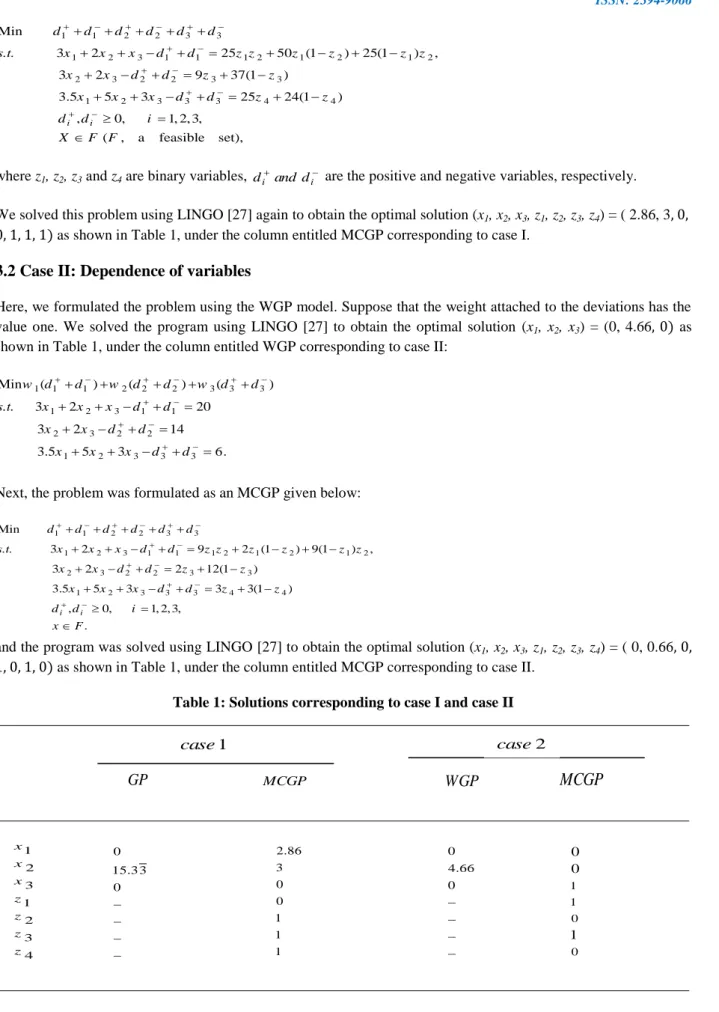
3.2 Case II: Dependence of variables
Here, we formulated the problem using the WGP model. Suppose that the weight attached to the deviations has the value one. We solved the program using LINGO [27] to obtain the optimal solution (x1, x2, x3) = (0, 4.66, 0) as shown in Table 1, under the column entitled WGP corresponding to case II:
1 1 1 2 2 2 3 3 3 1 2 3 1 1 2 3 2 2 1 2 3 3 3 Min ( ) ( ) ( ) 3 2 20 3 2 14 3.5 5 3 6. w d d w d d w d d s.t. x x x d d x x d d x x x d d
Next, the problem was formulated as an MCGP given below:
1 1 2 2 3 3 1 2 3 1 1 1 2 1 2 1 2 2 3 2 2 3 3 1 2 3 3 3 4 4 Min 3 2 9 2 (1 ) 9(1 ) , 3 2 2 12(1 ) 3.5 5 3 3 3(1 ) , 0, 1, 2, 3, . i i d d d d d d s.t. x x x d d z z z z z z x x d d z z x x x d d z z d d i x F
and the program was solved using LINGO [27] to obtain the optimal solution (x1, x2, x3, z1, z2, z3, z4) = ( 0, 0.66, 0,
1, 0, 1, 0) as shown in Table 1, under the column entitled MCGP corresponding to case II.
Table 1: Solutions corresponding to case I and case II 1 case
GP
MCGP 1 2 3 1 2 3 4 x x x z z z z 0 15.3 3 0 2.86 3 0 0 1 1 1 2 caseWGP
MCGP
0 4.66 0 1 1 0 0 0 0 1Journal of Information Sciences and Computing Technologies(JISCT) ISSN: 2394-9066 Table 2 and Table 3 respectively give summaries of the results obtained from the GP and MCGP models.
As seen in Table 2, MCGP has the total deviation value of 9.43 which is obviously better than the total deviation value of 97 obtained by the GP model. From Table 2, we realize that Goal 1 has achieved 31 percent of the aspiration level 100, Goal 2 has reached the aspiration level 46 exactly, andGoal 3 has reached 64 percent of the aspiration level 49, in the GP model of case I. However, we can see from Table 2 that these values are different by applying the MCGP model, and solutions of the MCGP is better than those of GP, because the percentage of goal achievement obtained from the MCGP model is better than the GP model. In other words, the more aspiration levels, the better the solutions.
Table 2: Comparison of GP and MCGP models in case I
From Table 3, MCGP has the total deviation value of 1 which is better than the number 28 obtained by the GP model in case II. As can be seen from Table 3, Goal 1 has reached 47 percent of the aspiration level 20, from GP model of case II. Goal 2 has reached the aspiration level 14 exactly, and Goal 3 has reached 26 percent of the aspiration level 6. As we seen from Table 3, percentage of goal achievement by the MCGP model is better than the ones by the GP model.
Table 3: Comparison of GP and MCGP models in case II
4. Conclusions
A new approach for solving the MODM problem with multiple utility functions was presented. While existing studies have considered MODM problems with the objective function having a single utility function, here we considered probabilities of multiple utility functions as aspiration levels of goal programming (GP) or multi-choice goal programming (MCGP) models. We worked through a simple example in order to show the usefulness of the proposed approach. The results showed that the solution of the MCGP model is better than that of the GP model for the DM. Because the solution of the MCGP model balance on the overall goals, better aspiration levels are obtained by applying the MCGP model.
GP
(%) percentage of goal achievement (%) percentage of goal achievementMCGP
31 46 76.65 97 2 3 1 Goal Goal Goal T otal deviation 31 100 64 15 9 25 9.43 60 100 100GP
percentage of goal achievement (%) percentage of goal achievement (%) MCGP 9.32 14 23.3 28 1 2 3 Goal Goal Goal T otal deviation 47 100 26 1.32 1.98 3.3 1 66 100 91Journal of Information Sciences and Computing Technologies(JISCT) ISSN: 2394-9066
References
[1] Romero, C., Sutclie, C., Board, J. and Cheshire, P. (1985). Naive weighting in non pre-emptive goal programming. viewpoint and reply. Journal of the Operational Research Society 36, 647–9.
[2] Charnes, A., Cooper, W.W. and Ferguson, R.O. (1955). Optimal estimation of executive compensation by linear Programming. Management Science 1, 138–151.
[3] Charnes, A. and Cooper, W.W. (1961). Management Model And Industrial Application of Linear Programming, John Wiley and Sons.
[4] Lee, S. M. (1972). Goal Programming for Decision Analysis. Philadelphia, PA, Auerbach. [5] Ignizio, J.P. (1985). Introduction to Linear Goal Programming. Beverly Hills, CA, Sage.
[6] Tamiz, M., J.D. and Romero, C. (1998). Goal programming for decision making : an overview of the current state-of-the-art. European Journal of Operational Research 111, 567–81.
[7] Romero, C. (2001). Extended lexicographic goal programming: a unifying approach. Omega 29, 63–71. [8] Chang, C.-T. (2007). Multi-choice goal programming. Omega 35, 389–396.
[9] Chang, C.-T. (2008). Revised multi-choice goal programming. Applied Mathematical Modeling 32, 2587–2595. [10] Chang, C-T. (2004). On the mixed binary goal programming problems. Applied Mathematics and Computation
159, 759–68.
[11] Vitoriano B. and Romero, C. (1999). Extended interval goal programming. Journal of Operational Research Society 50, 1280–3.
[12] Tamiz, M., Jones, D.F. and El-Darzi, E. (1993). A review of goal programming and its applications. Annals of Operations Research 58, 395–3.
[13] Flavell, R.B. (1976). A new goal programming formulation. Omega 4, 731–732.
[14] Zimmerman, H.J. (1983). Using fuzzy sets in operational research. European Journal of Operational Research 13, 201–206.
[15] Romero, C. (1991). Handbook of Critical Issues in Goal Programming. Pergamon Press, Oxford.
[16] Kluyver, C.A. (1979). De An exploration of various goal programming formulations with application to advertising media scheduling. Journal of the Operational Research Society 30, 167–171.
[17] Wildhelm, W.B. (1981). Extensions of goal programming models. Omega 9, 212–214.
[18] Jones, D.F. (1995). The Design and Development of an Intelligent Goal Programming System. Ph.D. Thesis, University of Portsmouth, UK.
[19] Masud, A.S. and Hwang, C.L. (1981). Interactive sequential goal programming, Journal of the Operational Research Society 32, 391–400.
[20] Wierzbicki, A. P. (1982). A mathematical basis for satisficing decision making. Mathematical Modelling 3, 391–405.
[21] Liao, C.-N. (2009). Formulating the multi-segment goal programming. Computer & Industrial Engineering 56, 138–141.
[22] Al-Nowaihi, A., Bradley, I. and Dhami, S. (2008). A note on the utility function under prospect theory. Economics Letters 99, 337–339.
[23] Yu, B.W.-T., Pang, W.K., Troutt, M.D. and Hou, S.H. (2009). Objective comparisons of the optimal portfolios corresponding to different utility functions. European Journal of Operational Research 199, 604–610.
[24] Podinovski, V.V. (2010). Set choice problems with incomplete information about the preferences of the decision maker. European Journal of Operational Research 207, 371–379.
[25] Chang, C.T. (2011). Multi-choice goal programming with utility functions. European Journal of Operational Research 215, 439–445.
[26] Olshausen, B. (2004). Bayesian Probability Theory. University of California, Berkeley. [27] Scharge, L. (2008). LINGO Release 11.0. LINDO System, Inc.
Journal of Information Sciences and Computing Technologies(JISCT) ISSN: 2394-9066 [28] Chang, C.-T., Chen, H.-M. and Zhuang, Z.-Y. (2012). Multi-coefficients goal programming. Computers &
Industrial Engineering 62, 616–623.
[29] Kettani, O., Aouni, B. and Martel, J.M. (2004). The double role of the wight factor in the goal programming model. Computer & Operational Research 31, 1833-1845.