Optimal Water System Operation Using Graph Theory Algorithms

(1)

Procedia Engineering 89 ( 2014 ) 502 – 508

Peer-review under responsibility of the Organizing Committee of WDSA 2014 doi: 10.1016/j.proeng.2014.11.245

ScienceDirect

16th Conference on Water Distribution System Analysis, WDSA 2014

Optimal Water System Operation Using Graph Theory Algorithms

E. Price

a,

*, A. Ostfeld

a

a_{Civil and Environmental Engineering, Technion—Israel Institute of Technology, Israel}

Abstract

The water system minimum-cost flow problem is solved using the successive shortest path (SSP), graph theory algorithm, by representing the network as a directed graph. The graph nodes represent water sources, junctions, tanks and consumers. The edges represent pipes, pumping stations water tanks. The successive shortest path algorithm is applied to the graph ending when max flow limitation is fulfilled between the sources and sink nodes, returning minimal operating costs. A simple 24h water system is examined using the proposed graph representation. The results are compared to the results of numeration and standard linear programing solver.

Peer-review under responsibility of the Organizing Committee of WDSA 2014. Keywords: Graph theory ; Water system ; optimal operation ; Pump scheduling ; Headloss

1. Introduction

Water system optimal operation is commonly solved using algebraic optimization models, such as linear, non-linear or mixed integer programing. In addition, evolutionary algorithms may be used such as genetics, ant colony and many others. This research proposes to solve the optimization problem using graph theory. The water balance optimization problem is represented as a directed graph on which graph theory algorithms may be applied. A simple SSP algorithm is demonstrated and compared to a classic linear programing (LP) solver. Many minimum-cost flow algorithms excise such as the Out-of-Kilter algorithm [2], the Cycle Cancelling algorithm [4], dual Successive Shortest Path [6] and many modifications and others [1].

This research solves water system optimization operation problem using graph theory. Commonly the problem is solved using algebraic optimization problems, such as linear, non-linear or mixed integer programing. In addition,

* Corresponding author. Tel.: +972-3-6924603; fax: +972-3-6924550. E-mail address: [email protected]

(2)

evolutionary algorithms may be used such as genetics, ant colony and many others. The optimization problem is represented as a directed graph problem: The nodes represent water sources, junctions and consumers and the edges represent consumer demand constraints and water tanks passing water from one time step to the next. The water balance problem is solved using the successive shortest path algorithm. The SSP results are compared to a classic linear programing solver. Other minimum-cost flow algorithms excise and may be used such as Out-of-Kilter algorithm [2], Cycle Cancelling algorithm [4], dual Successive Shortest Path [6] and many modifications and others [1].

Nomenclature

d demand node index

D subset of all demand type nodes within set N

E set of all arc (edge) indexes in examined water system

i, j, k index of origin and destination nodes

N set of all nodes in examined water system

p pump station node index

P subset of all pump type nodes within set N

Qp

max maximum nominal pump station flow rate, constant (m3/h)

Qt

i,j flow rate in pipe, variable (m3/h)

r water tank index

R subset of all water tank type nodes within set N

t time index (hr)

T set of all time indexes (0…23)

Tarpt hourly electrical tariff charge (NIS/kWh)

THp pumps total head, constant (m), 70m

Vrmax water tank water maximum volume, constants (m3)

Vrmin water tank water minimum volume, constants (m3)

Vrt water volume in water tank, variable (m3)

γ unit conversion, constant (γ = 0.736 / 270)

ηp pump’s overall efficiency (pump, motor and mechanical losses), constant, 75%

2. Methodology

2.1 Examined water system

The examined water system is presented in Fig. 1, used by [5]. A pumping station [P], with a nominal flow rate of

1,000 m3_{/h and a total head of 70 m, pumps water from a water source [S] to a water tank [T]. The water tank has an}

operational volume of 5,000 m3_{and at the end of the day must return to the daily starting volume. Consumer [D] has}

an hourly water demand of 900 m3_{/h, during 10 hours (between hours 7 to 16, total of 9,000 m}3_{/day) and may be}

supplied from the water tank or from the pumping station. The electrical tariff rate (c) is 0.2768 NIS/kWh between hours 0 to 6 and 21 to 23, 0.4316 NIS/kWh between hours 7 to 9 and 17 to 20, 1.0089 NIS/kWh between hours 10 to 16. The pump has a fixed total head (TH) of 70 m, a total efficiency of 75% and a constant energy consumption (E) of 0.254 kWh/ m3_.

(3)

Fig 1. Example water distribution system, algebraic form

2.2 Linear programming

The 24-hour period water system, was solved using GAMS/CLP (open-source linear programming solver). The minimum cost objective function is presented in Eq. (1), and the water balance constraints are presented in Eq. (2) to (6). The linear problem was defined using the minimum cost objective function in Eq. (1). and the constraints in equations (2) to (6).

Minimize annual operation cost (objective function):

» ¼ º « ¬ ª u u u u

¦¦

T t P p p p t j p TH Q 1 1 1 t p , Tar min K J (1)

Water balance at nodes:

i

j

k

E

t

T

Q

N k t k j N i t j i

¦

, ,

,

;

,

(2)

Demand node water balance:

,

N t t i d d i

Q

De

d D

t T

¦

(3)

Pump node input:

max ,

,

N t i p p i

Q

d

Q

i p

E

t T

¦

(4)

Water tank hourly and daily water balance:

1 , ,

, ; ,

,

N N t t t t r r i r r j i j

V

¦

Q

¦

Q

i r r j

E

r R

t T

_(5a)

0 23 0 0 , ,

, ; ,

,

N N t t t t r r i r r j i j

V

¦

Q

¦

Q

i r r j

E

r R

(5b) [s] Legend Q = Flow (m3_/hr) TH = Total head (m)

V = water tank max volume (m3₎

[s] = Source node [p] = Pump edge [j] = Junction node [t] = Water tank node [d] = Consumer demand node Node [r] [d] [j] [p] Q=1000 TH=70 Q=900 V=5000

(4)

Water min/max water tank volume constraint:

min t max

r r r

V

d

V

d

V

(6)

2.3 Directed graph

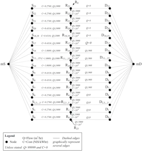
The examined water system was modelled as a directed graph and was solved using the successive shortest path algorithm (SSP), see Fig. 2.

Fig 2. Example water distribution system, directed graph form

The nodes and edges of the hourly time step water system representation in Fig. 1, are multiplied 24 times and stacked one on the other. A master daily water source is represented as node [mD], from this node water is logically supplied to each of the hourly water sources [St]. Each of the hourly water sources [St] is connected to a water tank node [Rt] and on to the hourly consumer node [Dt]. The accumulated daily water demand flows from the demand nodes [Dt] to a master demand node [mD]. Each water tank node [Rt] is connected to the following water tanks allowing from water to flow from one time step [Rt] to the next [Rt+1]. The flow in edges [St-Rt] is limited to 1000 m3_{/h and has a flow cost matching the hourly electrical tariff [Ct]. The flow in edges [Rt-Dt] is limited to zero if no} if there is no hourly water consumption or to 900 m3_{/h during consumption hours. The flow in the edges [Rt-Rt+1] is}

mS mD S0 R0 D0 S1 R1 D1 R2,3..,5 R23 Q≤900 S6 R6 D6 S7 R7 D7 S8 R8 D8 R10 D10 S10 S9 R9 D9 R11,..,15 Q≤900 R16 D16 S17 D17 S16 S11,..,15 D11,..,15 R17 Q≤900 S18,19 R18,19 D18,19 S20 R20 D20 R22 D22 S23 D23 R0 S22 S21 R21 D21 R23 Q≤900 Q=0 Q=0 Q=0 Q=0 Q=0 Q≤0 Q≤0 Q≤0 C=0.2768;Q≤1000 C=0.2768;Q≤1000 C=0.2768;Q≤1000 C=0.4316;Q≤1000 C=0.4316;Q≤1000 C=1.0089;Q≤1000 C=1.0089;Q≤1000 C=0.4316;Q≤1000 C=0.4316;Q≤1000 C=0.2768;Q≤1000 C=0.2768;Q≤1000 C=0.2768;Q≤1000 S2,3,..,5 D2,3,..,5 Q≤900 C=0.4316;Q≤1000 Q≤900 C=1.0089;Q≤1000 C=0.4316;Q≤1000 Q=0 C=0.2768;Q≤1000 Q≤0 Legend Legend Node Node Q=Flow (m 3_/hr) C=Cost (NIS/kWhr) Q=Flow (m3_/hr) C=Cost (NIS/kWhr) Q≤5000 C=10-6 Un U

U less stated: Q<99999 and C=0

Unless stated: Q<99999 and C=0

Q≤5000 C=10-6 Q≤5000 C=10-6 Q≤5000 C=10-6 Q≤5000 C=10-6 Q≤5000 C=10-6 Q≤5000 C=10-6 Q≤5000 C=10-6 Q≤5000 C=10-6 Q≤5000 C=10-6 Q≤5000 C=10-6 Q≤5000 C=10-6 Q≤5000 C=10-6 Q≤5000 C=10-6 Q≤5000 C=10-6 Q≤5000 C=10-6 Dashed edgd es gr

gg apa hicallyll repe resent

several edgd es

Dashed edges graphically represent several edges

(5)

limited to 5000 m3_{/h, meaning that no more than 5,000 m}3_{may be passed from one hour to the next, equivalent to} the water tank’s maximum volume. A constant flow cost (C) exists along the water tank nodes, encouraging the model to minimize the amount of water passed between the water tank nodes, minimizing the time the water is held in the water tanks, reducing water age. Note that node [R23] is connected to node [R0] allowing for water to pass from the end of the day the beginning of the following day, assuming the system is daily steady state and enforcing the constraint that the water in the water tank must return to the daily starting volume at the end of the day.

2.4 Successive shortest path algorithm

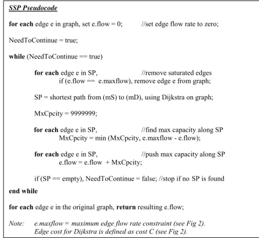
The successive shortest path algorithm (SSP) passes maximum flow from [mS] to [mD], with minimum cost. The pseudo code used to solve the directed graph form is presented in Fig. 3.

Fig. 3. Successive shortest path algorithm, Pseudocode

In the first iteration, the edges with a maximum flow rate of zero (consumer edges with no hourly consumption) are removed as no flow will pass through them. Using Dijkstra [3], a shortest path is found from [mS] to [mD], shortest path is defined as min(∑Qij*Cij), edge cost is defined by C in Fig. 2. Next, a maximum residual capacity flow rate is pushed along the shortest found path. Next, edges, which have reached their maximum flow rate capacity, are removed from the graph. The algorithm repeats until no more paths are found between [mD] and [mS], meaning maximum flow constraints are reached.

SSP Pseudocode

for each edge e in graph,set e.flow = 0; //set edge flow rate to zero; NeedToContinue = true;

while (NeedToContinue == true)

for each edge e in SP, //remove saturated edges if (e.flow == e.maxflow), remove edge e from graph; SP = shortest path from (mS) to (mD), using Dijkstra on graph; MxCpcity = 9999999;

for each edge e in SP, //find max capacity along SP MxCpcity = min (MxCpcity, e.maxflow - e.flow); for each edge e in SP, //push max capacity along SP

e.flow = e.flow + MxCpcity;

if (SP == empty), NeedToContinue = false; //stop if noSP is found

end while

for each edge e in the original graph, return resulting e.flow; Note: e.maxflow = maximum edge flow rate constraint (see Fig 2).

(6)

3. Results 3.1 Examined cases

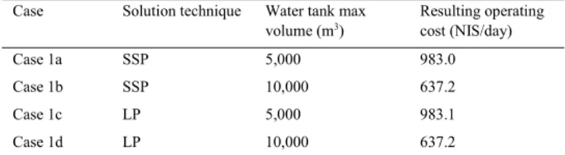
Several cases were solved using LP and SSP, as presented in table 1. The optimal operation cost were found for a water tank with a volume of 5,000 m3_{, and 10,000 m}3_.

Table 1. Examined cases and results of successive shortest path and linear programing Case Solution technique Water tank max

volume (m3₎ Resulting operating cost (NIS/day) Case 1a SSP 5,000 983.0 Case 1b SSP 10,000 637.2 Case 1c LP 5,000 983.1 Case 1d LP 10,000 637.2 3.2 Comparing results

The resulting daily operating cost is presented in Table 1. The resulting minimal operating costs of the system found by the SSP and the LP models are the same, 983.1 NIS and 637.2 NIS, respectively (assuming that the minor difference in the operating cost of case 1a and 1c is due to numerical error). Enlarging the water storage in the water tanks lowers the operational costs of the system as more water may be pumped to the water tanks during low tariff rate hours, and supplied gravitationally from the water tank to consumption during peak electrical tariff hours.

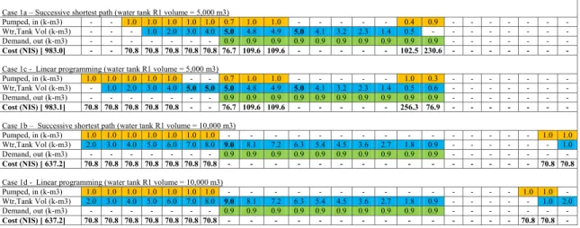
Fig. 4 presents a detailed data for the optimal pump scheduling found. In comparison to the LP results, the SSP results minimizes the number of hours the water tanks hold water, minimizing the water age supplied to the consumers and grouping pump operation to consecutive hours. This is due to the flow cost penalty along the reservoir edges minimizing the number of reservoir edges used. For example in case 1c (LP) the water tank is filled

from hour 1 and is held full at 5,000 m3_{for 3 hours during hour 5 to hour 7, with no consumption, while in case 1a}

(SSP) the tank starts to fill from hour 3 and reaches maximum volume in hour 7 as consumption starts. The same may be seen in case 1d (LP) as the tank is filled during hour 22 and in case 1b (SSP) is filled in hour 23. Both LP

and SSP use only 9,000 m3 of the available 10,000 m3_{water volume in the water tank, in cases 1b and 1d.}

4. Conclusions

A pump scheduling optimal operation problem was solved using successive shortest path graph theory algorithm. The results were compared to the solution of the problem using linear programing and algebraic constraints. Both solution methods returned the same optimal operation cost and similar pump scheduling. Using SSP, a flow cost fine in the reservoir edges caused the water to be held for fewer hours in the water tanks before consumption, relative to the LP water tank operation, improving water age and by such water quality to consumers. SSP grouped pump operating hours, allowing for longer and consecutive pump operation with less pump activations, relative to the sporadic like pump operation of the LP solver. Further research it is proposed to include non-linear hydraulic and pump curve constraints to be solved using graph theory algorithms.

5. Acknowledgements

This study was supported by the joint Israeli Office of the Chief Scientist (OCS) Ministry of Industry, Trade and Labor (MOITAL), and by the Germany Federal Ministry of Education and Research (BMBF), under project number GR_2443.

(7)

Fig. 4. Hourly results of successive shortest path and linear programing

References

[1] T. Brunsch, K. Cornelissen, B. Manthey, H. Röglin, Smoothed analysis of the successive shortest path algorithm, in: Proceedings of the 12th Cologne-Twente Workshop on Graphs and Combinatorial Optimization, Centre for Telematics and Information Technology, University of Twente. (2013) 27-30.

[2] R.F. Delbert , An out-of-kilter algorithm for minimal cost flow problems, Journal of the SIAM, 9 (1961) 18-27. [3] E.W. Dijkstra, A note on two problems in connection with graphs, in: Numerische Mathematik 1 (1959) 269–271.

[4] K. Morton, A primal method for minimal cost flows with applications to the assignment and transportation problems, Management Science, 14 (1967) 205-220.

[5] E. Price, A. Ostfeld, Discrete Pump Scheduling and Leakage Control Using Linear Programming for Optimal Operation of Water Distribution Systems, Journal of Hydraulic Engineering, (2014) DOI: 10.1061/(ASCE)HY.1943-7900.0000864.

[6] S.J. William, Optimal flow through networks, Operations Research, 10 (1962) 476-499.

* For all cases: total pump efficiency = 75%, pump total head = 70m, pump energy consumption = 0.254 kW/m3. Presented water tank volume is at the beginning of the hour.

Hour of day (hr) 0 1 2 3 4 5 6 7 8 9 10 11 12 13 14 15 16 17 18 19 20 21 22 23

Tariff (NIS/kWhr) 0.28 0.28 0.28 0.28 0.28 0.28 0.28 0.43 0.43 0.43 1.01 1.01 1.01 1.01 1.01 1.01 1.01 0.43 0.43 0.43 0.43 0.28 0.28 0.28 Case 1a – Successive shortest path (water tank R1 volume = 5,000 m3)

Pumped, in (k-m3) - - 1.0 1.0 1.0 1.0 1.0 0.7 1.0 1.0 - - - 0.4 0.9 - - - - Wtr,Tank Vol (k-m3) - - - 1.0 2.0 3.0 4.0 5.0 4.8 4.9 5.0 4.1 3.2 2.3 1.4 0.5 - - - - Demand, out (k-m3) - - - 0.9 0.9 0.9 0.9 0.9 0.9 0.9 0.9 0.9 0.9 - - - -

Cost (NIS) [983.0] - - 70.8 70.8 70.8 70.8 70.8 76.7 109.6 109.6 - - - - - 102.5 230.6 - - - - - - -

Case 1c - Linear programming (water tank R1 volume = 5,000 m3)

Pumped, in (k-m3) 1.0 1.0 1.0 1.0 1.0 - - 0.7 1.0 1.0 - - - 1.0 0.3 - - - - Wtr,Tank Vol (k-m3) - 1.0 2.0 3.0 4.0 5.0 5.0 5.0 4.8 4.9 5.0 4.1 3.2 2.3 1.4 0.5 0.6 - - - - Demand, out (k-m3) - - - 0.9 0.9 0.9 0.9 0.9 0.9 0.9 0.9 0.9 0.9 - - - -

Cost (NIS) [ 983.1] 70.8 70.8 70.8 70.8 70.8 - - 76.7 109.6 109.6 - - - - - 256.3 76.9 - - - - - - -

Case 1b – Successive shortest path (water tank R1 volume = 10,000 m3)

Pumped, in (k-m3) 1.0 1.0 1.0 1.0 1.0 1.0 1.0 - - - 1.0 1.0 Wtr,Tank Vol (k-m3) 2.0 3.0 4.0 5.0 6.0 7.0 8.0 9.0 8.1 7.2 6.3 5.4 4.5 3.6 2.7 1.8 0.9 - - - 1.0 Demand, out (k-m3) - - - 0.9 0.9 0.9 0.9 0.9 0.9 0.9 0.9 0.9 0.9 - - - -

Cost (NIS) [ 637.2] 70.8 70.8 70.8 70.8 70.8 70.8 70.8 - - - - - - - - - - - - - - - 70.8 70.8

Case 1d - Linear programming (water tank R1 volume = 10,000 m3)

Pumped, in (k-m3) 1.0 1.0 1.0 1.0 1.0 1.0 1.0 - - - 1.0 1.0 - Wtr,Tank Vol (k-m3) 2.0 3.0 4.0 5.0 6.0 7.0 8.0 9.0 8.1 7.2 6.3 5.4 4.5 3.6 2.7 1.8 0.9 - - - 1.0 2.0 Demand, out (k-m3) - - - 0.9 0.9 0.9 0.9 0.9 0.9 0.9 0.9 0.9 0.9 - - - -