Prediction of Protein Secondary
Structure using Binary Classification
Trees, Naive Bayes Classifiers and the
Logistic Regression Classifier
A thesis submitted in partial fulfillment of the requirements for the degree of
MASTER OF SCIENCE
in the
DEPARTMENT OF STATISTICS
of
RHODES UNIVERSITY
by
Ahmed Abdelkarim Eldud Omer
Abstract
The secondary structure of proteins is predicted using various binary classifiers. The data are adopted from the RS126 database. The original data consists of protein primary and secondary structure sequences. The original data is encoded using alphabetic letters. These data are encoded into unary vectors comprising ones and zeros only. Different binary classifiers, namely the naive Bayes, logistic regression and classification trees using hold-out and 5-fold cross validation are trained using the encoded data. For each of the classifiers three classification tasks are considered, namely helix against not helix (H/∼H), sheet against not sheet (S/∼S) and coil against not coil (C/∼C). The performance of these binary classifiers are compared using the overall accuracy in predicting the protein secondary structure for various window sizes.
Our result indicate that hold-out cross validation achieved higher accuracy than 5-fold cross validation. The Naive Bayes classifier, using 5-fold cross validation achieved, the lowest accu-racy for predicting helix against not helix. The classification tree classifiers, using 5-fold cross validation, achieved the lowest accuracies for both coil against not coil and sheet against not sheet classifications. The logistic regression classier accuracy is dependent on the window size; there is a positive relationship between the accuracy and window size. The logistic regression classier approach achieved the highest accuracy when compared to the classification tree and Naive Bayes classifiers for each classification task; predicting helix against not helix with accu-racy77.74%, for sheet against not sheet with accuracy81.22%and for coil against not coil with accuracy 73.39%. It is noted that it is easier to compare classifiers if the classification process could be completely facilitated in R. Alternatively, it would be easier to assess these logistic regression classifiers if SPSS had a function to determine the accuracy of the logistic regression classifier.
Keywords: Classification tree, Naive Bayes, logistic regression, hold-out,5-fold cross validation, protein secondary structure prediction
Contents
Abstract i
List of Tables vi
List of Figures viii
1 Outline 1
1.1 Framework . . . 1
1.2 Research Background . . . 1
1.3 Goal of the Research . . . 2
1.4 Introduction . . . 2
2 Classification 3 2.1 Introduction . . . 3
2.2 Classification . . . 3
2.3 Measurement of Classifier Accuracy . . . 4
2.4 Measurement of Binary Classifier Accuracy . . . 6
2.5 Cross Validation . . . 9
2.5.1 k-fold Cross Validation . . . 10
2.5.2 Hold-Out Cross Validation . . . 11
2.5.3 Leave-One-Out Cross Validation . . . 12
3 Classification Using the Naive Bayes and Logistic Regression Classifiers 15 3.1 Introduction . . . 15
3.2 Classifiers Based on Bayes Rule . . . 15 iii
3.2.2 Estimating the Likelihood . . . 17
3.3 Naive Bayes Classifier . . . 18
3.3.1 Estimating the Maximum Likelihood for Naive Bayes Classifier . . . 19
3.4 Logistic Regression . . . 20
3.4.1 The Logistic Regression Model . . . 20
3.4.2 Estimation of the Logistic Regression Model Parameters . . . 23
3.4.2.1 The Newton Raphson Method . . . 25
3.4.3 Using Logistic Regression as a Classifier . . . 28
4 Classification Trees 31 4.1 Introduction . . . 31
4.2 Binary Classification Trees . . . 31
4.3 Impurity Functions . . . 32 4.3.1 Node Impurity . . . 32 4.3.2 Tree Impurity . . . 33 4.4 Splitting Rules . . . 34 4.4.1 Gini Index . . . 34 4.4.2 Entropy Index . . . 38 4.5 Splitting Procedure . . . 39 4.5.1 Maximum Tree . . . 40 4.6 Pruning a Tree . . . 41
4.6.1 Cost Complexity Pruning . . . 41
4.7 Cross Validation . . . 45
5 Prediction of the Protein Secondary Structure 47 5.1 Introduction . . . 47
5.2 Proteins and Amino Acids . . . 47
5.3 Protein Structure and Function . . . 49
5.4 Secondary Structure Prediction . . . 50
5.6 Prediction of Protein Secondary Structure using Classification Trees . . . 55
5.6.1 Hold-Out Classification . . . 55
5.6.1.1 Data Set Partition and Application . . . 55
5.6.1.2 Classification Tree Accuracy Using Hold-Out Cross Validation 55 5.6.2 5-fold Cross Validation . . . 56
5.6.2.1 Data Set Partition and Application . . . 56
5.6.2.2 Classification Tree Accuracy Using 5-fold Cross Validation . . . 57
5.7 Prediction of Protein Secondary Structure using Naive Bayes Classifiers . . . 58
5.7.1 Hold out classification . . . 58
5.7.1.1 Data Set Partition and Application . . . 58
5.7.1.2 Naive Bayes Classifier Accuracy Using Hold-Out Cross Validation 58 5.7.2 5-fold Cross Validation . . . 60
5.7.2.1 Data Set Partition and Application . . . 60
5.7.2.2 Naive Bayes Classifier Accuracy using 5-fold Cross Validation . 60 5.8 Prediction of Protein Secondary Structure using Logistic Regression Classifiers . 61 5.8.1 Hold-Out Cross Validation . . . 61
5.8.1.1 Data Set Partition and Application . . . 61
5.8.1.2 Logistic Regression Classifier Accuracy . . . 62
5.8.2 5-fold Cross Validation . . . 63
5.8.2.1 Data Set Partition and Application . . . 63
5.8.2.2 Logistic Regression Classifier Accuracy Using 5-fold Cross Val-idation . . . 63
5.9 Comparison of the Naive Bayes, Classification Tree and Logistic Regression Clas-sifiers . . . 65
5.9.1 Helix against not Helix . . . 65
5.9.2 Coil against not Coil . . . 67
5.9.3 Sheet against not Sheet . . . 70
6 Conclusion 75 6.1 Introduction . . . 75
6.2 Conclusions and Discussion . . . 75
Appendix A Classification Trees: Hold-Out Cross Validation 83
Appendix B Classification Trees: 5-fold Cross Validation 87
Appendix C Naive Bayes: Hold-Out Cross Validation 93
Appendix D Naive Bayes: 5-fold Cross Validation 97
Appendix E Logistic Regression: Hold-Out Cross Validation 101
Appendix F Logistic Regression: 5-fold Cross Validation 103
List of Tables
2.1 Possible outcomes of the classification of a binary variable. . . 6
2.2 A confusion matrix for the classification of n binary observations. . . 7
2.3 10-fold cross validation (iteration process). . . 11
2.4 Hold-out cross validation. . . 12
2.5 Leave one out cross validation. . . 13
4.1 Classification table: The binary split of Y for variable xj. . . 31
4.2 The Gini split and goodness of the split in the non-terminal nodes in the tree depicted in figure 4.4.2. . . 38
4.3 The Entropy split and goodness of the split in the non-terminal nodes in the tree depicted in figure 4.4.2. . . 39
5.1 Amino acid abbreviations. . . 48
5.2 The actinoxanthin (1acx.concise) entry in the RS126 data set. . . 51
5.3 The amino acid encoding matrix. . . 52
5.4 The secondary structure encoding. . . 52
5.5 The first four observations of the actinoxanthin (1acx.concise) sequence as con-sidered in this study. . . 53
5.6 Encoding of the actinoxanthin (1acx.concise) entry for a window of size 3. . . 53
5.7 Test accuracy (%) of the classification trees. . . 56
5.8 Test accuracy (%) of the classification trees using 5-fold cross validation. . . 57
5.9 Test accuracy (%) of the Naive Bayes classifier. . . 59
5.10 Test accuracy (%) of the Naive Bayes classifiers using 5-fold cross validation. . 60
5.11 Test accuracy (%) of the logistic regression classifier. . . 63 5.12 Test accuracy (%) of the logistic regression classifier using 5-fold cross validation. 64
for the Naive Bayes, classification tree and logistic regression classifiers using hold-out or5-fold cross validation. . . 65 5.14 Summary of the test accuracy (%), amoungst all window sizes, when
predict-ing helix against not helix for the Naive Bayes, classification tree and logistic regression classifiers using hold-out or 5-fold cross validation. . . 66 5.15 Test accuracy (%), for all window sizes, when predicting coil against not coil
for the Naive Bayes, classification tree and logistic regression classifiers using hold-out or5-fold cross validation. . . 68 5.16 Summary of the test accuracy (%), amoungst all window sizes, when predicting
coil against not coil for the Naive Bayes, classification tree and logistic regression classifiers using hold-out or 5-fold cross validation. . . 68 5.17 Test accuracy (%), for all window sizes, when predicting sheet against not sheet
for the Naive Bayes, classification tree and logistic regression classifiers using hold-out or5-fold cross validation. . . 71 5.18 Summary of the test accuracy (%), amoungst all window sizes, when
predict-ing sheet against not sheet for the Naive Bayes, classification tree and logistic regression classifiers using hold-out or 5-fold cross validation. . . 71 6.1 Comparison of the effect of change in window size on logistic regression and
support vector machine Hua and Sun (2001). . . 76 6.2 Comparison of the logistic regression result with support vector machine using
List of Figures
3.4.1 Odds, logit and probability . . . 22
4.2.1 A figure depicting the root node, non-terminal and terminal nodes of a classifi-cation tree. . . 32
4.4.1 Binary split the node t1. . . 36
4.4.2 An example of a binary tree. . . 37
4.6.1 The maximum tree, T0. . . 42
4.6.2 Sub-tree T1. . . 43
4.6.3 Sub-tree T3. . . 43
4.6.4 Sub-tree T1. . . 44
4.6.5 Sub-tree T2. . . 45
4.6.6 Sub-tree T4. . . 45
5.2.1 An example of a protein amino acid structure. . . 48
5.2.2 The four levels of protein structure (From Boundless, 2014). . . 49
5.5.1 Creating the data set for a window of size 3 (From Baxter and Jäger, 2011). . . 54
5.6.1 Test accuracy (%) of the classification trees. . . 55
5.6.2 Test accuracy (%) of the classification trees using 5-fold cross validation. . . 57
5.7.1 Test accuracy (%) of the Naive Bayes classifier. . . 59
5.7.2 Test accuracy (%) of the Naive Bayes classifier using 5-fold cross validation. . . 61
5.8.1 Test accuracy (%) of the logistic regression classifier. . . 62
5.8.2 Test accuracy (%) of the logistic regression classifier using 5-fold cross validation. 64 5.9.1 Comparison of the test accuracies (%) for predicting helix against not helix for each of the Naive Bayes, classification tree and logistic regression classifiers using hold-out or5-fold cross validation. . . 66
dicting helix against not helix for each of the Naive Bayes, classification tree and logistic regression classifiers using 5-fold cross validation. . . 67 5.9.3 Comparison of the test accuracies (%) for predicting coil against not coil for
each of the Naive Bayes, classification tree and logistic regression classifiers using hold-out or5-fold cross validation. . . 69 5.9.4 Heuristic confidence intervals: Comparison of the test accuracies (%) for
pre-dicting coil against not coil for each of the Naive Bayes, classification tree and logistic regression classifiers using hold-out or5-fold cross validation. . . 70 5.9.5 Comparison of the test accuracies (%) for predicting sheet against not sheet for
each of the Naive Bayes, classification tree and logistic regression classifiers using hold-out or5-fold cross validation. . . 72 5.9.6 Heuristic confidence intervals: Comparison of the test accuracies (%) for
predict-ing sheet against not sheet for each of the Naive Bayes, classification tree and logistic regression classifiers using hold-out or5-fold cross validation. . . 73
Acknowledgments
I would like to thank my supervisor, Mr Jeremy Baxter, for the patient guidance, encouragement and advice he has provided throughout my time as his student. I have been extremely lucky to have a supervisor who cared so much about my work, and who responded to my questions and queries so promptly. I would like to thank Professor Sarah Radloff, for giving me a chance to be a student at Rhodes University, and also for her patient guidance and unwavering support through out my study.
I would also like to thank all the members of the Statistics Department at Rhodes University and also those at the University of the Western Cape for all the support they gave me through out my study.
I would also like to acknowledge the support I got from my friends.
Finally, I must express my very profound gratitude to my family especially my mother, brothers (Nasreldein, Mohamed and Ibrahim) and sisters for providing me with unfailing support and continuous encouragement throughout my years of study and through the process of researching and writing this thesis. This accomplishment would not have been possible without them. Thank you.
Chapter 1
Outline
1.1
Framework
This study considers how a researcher might predict the secondary structure of proteins based on the proteins primary structure. Statistical classification, measures of classifier accuracy and cross validation are introduced and discussed in chapter 2. Chapter 3 discusses how Bayes rule can be used to construct the Naive Bayes classifier and how logistic regression can be utilised to construct a classifier. Classification trees are defined and discussed in chapter 4. Chapter 5 describes the structure of proteins and how the data set used in this study was processed for supervised classification. The results of the various classifiers, using hold-out and 5-fold cross validation, are reported and discussed. These classifiers are compared in the context of this particular data set. Chapter 6 compares these results to those of other researchers. Appendices A to G contain the relevant R code used in this study.
1.2
Research Background
Protein secondary structure prediction is the prediction of the secondary structure of a protein based on the primary structure that is from the linear sequence of amino acids. The prediction of the secondary structure depends on the amino acids sequence. An aim of theoretical chemistry and bioinformatics is to predict the sequence of the protein structure from the primary structure (Zhang and Rajapakse, 2009). Some of the computationally based methods that can be used to predict the secondary predictions include Naive Bayes, logistic regression classifier, classification trees, neural networks, support vector machines and nearest neighbor methods (Singh et al., 2008).
1.3
Goal of the Research
The aim of this study is to predict the secondary structure of the proteins using three classifi-cation approaches, namely the classificlassifi-cation tree, Naive Bayes and logistic regression classifiers. This study assesses the performance of these classifiers using hold-out and 5-fold cross valida-tion. To achieve these objectives, R and SPSS are used to perform the calculations relevant to this study.
1.4
Introduction
The objective of this study is to train classification tree, Naive Bayes and logistic regression classifiers based on a sequence of protein primary structure in order to predict the proteins secondary structure. The data used in this study consist of 126 proteins available in the Rost and Sander database (Rost and Sander, 1993) available from http://www.anteprot-pbil. ibcp.fr/. As discussed in section 5.5, this data set contains the proteins name and the primary and secondary structure sequence of each protein.
The data processing is done in steps: The first step performed is pre-processing. The data is presented as letters and the purpose of pre-processing is to convert the letters into numbers. To achieve this, the orthogonal coding scheme (Holley and Karplus, 1989) is used. The second step is to assign the secondary structure. Secondary structures are classified into 8 categories, namely α-helix (H), 310-helix (G), π-helix (I), β-strand (E), isolated β-bridge (B), turn (T),
bend (S) and rest (-) where the last category is for unclassified structures. Section 5.5 indicates how these structures are reduced to 3categories, namely helix (H), sheet (E) and coil (C). SPSS and R, statistical software, are used to fit and assess the performance or accuracy of the various classifiers used in this study. Hold-out and 5-fold cross validation are used to estimate the performance of each of the classifiers, namely the classification tree (section 5.6), Naive Bayes (section 5.7) and logistic regression (section 5.8) classifiers. The classification tree, Naive Bayes and logistic regression classifiers are compared in section 5.9 using the overall accuracy measure as defined and discussed in section 2.4. These results are compared to those of other researchers in chapter 6.
Chapter 2
Classification
2.1
Introduction
Section 2.2 introduces classification in a mathematical context. Section 2.3 defines and dis-cusses various measures of classifier accuracy. Section 2.4 disdis-cusses these measures for binary classifiers. The cross validation approach to assessing classifier accuracy is discussed in section 2.5.
2.2
Classification
Classification is an important technique that is used in statistics. Classification is sometimes known as statistical pattern recognition or discrimination (Breiman et al., 1984). When mod-eling the relationship between the response variable denoted by y, and the predictor variable denoted by x= (x0, x1, x2, ..., xp)′, where xǫRp+1, the predictors may either be continuous or discrete random variables. If the response variable is continuous the modeling process is termed regression modeling. If the response variable is categorical the modeling process termed clas-sification modeling (Izenman, 2009; Han and Micheline, 2006). In clasclas-sification the response variable is labeled as belonging to one ofL classes. There is often no natural ordering to these classes, but they are labeled as 1,2, ..., L, where L is the number of classes. When there are more than two classes, that is when L >2,the modeling is called multi-class classification. This report focuses on binary variable classification, that is where there are two classes. The class labels are commonly taken to be yǫ{0,1}. It is assumed that the response variable is in-fluenced by the associated predictor variables,x. The classification is a conditional distribution where the response variable is binary, where p(y= 1|x) = 1−p(y= 0|x), and hence follows a Bernoulli distribution with parameter β, which denotes the probability of 1:
p(y|β) =βy(1−β)1−y where y= 0,1
The response or dependent variable is affected by the predictor or independent or feature or attribute variables, x= (x0, x1, x2, ..., xp)′ where p is the number of predictor or independent variables in the data set. Classification models can be used to predict the class of unknown observations. The goal is to build a model and use this model to predict which category a new subject or object belongs to. Thus the purpose of classification is to build a model which can be used for predicting the class label for an observation based on the values of the attributes or independent variables.
2.3
Measurement of Classifier Accuracy
There are several accuracy measures of classifier accuracy for instance specificity, sensitivity, misclassification and accuracy rate (Zaki and Meira Jr, 2014). Accuracy measures are de-signed to focus on specific aspects of a classifiers accuracy, for example the overall classification accuracy (Labatut and Cherifi, 2012; Foody, 2002).
Denote the true or observed class of an observation asyi and the associated observations of the independent or predictor variables asxi ∈Rp+1. Consider a classifier, denoted by M, which is simply a function or rule that assigns toxi a class label denoted by yˆi, that is
M :xi 7−→yˆi =f(xi)
LetI denote an indicator function that has value 1when the argument is true and0otherwise. For each observation (xi, yi) and associated predicted class label, yˆi, where i = 1, . . . , n, an indicator function can be used to denote a misclassification as follows
I(yi 6= ˆyi) = ( 1 if yˆi 6=yi 0 if yˆi =yi or a correct classification as I(yi = ˆyi) = ( 1 if yˆi =yi 0 if yˆi 6=yi
The error rate (Zaki and Meira Jr, 2014, page 603) or misclassification error rate is the fraction of incorrect predictions for the classifier over a data set. The error rate is defined in terms of the indicator function as
Error rate= 1 n n X i=1 I(yi 6= ˆyi)
5 2.3. Measurement of Classifier Accuracy The error rate is an estimate of the probability of misclassification and hence the lower the error rate the better the classifier. The accuracy of a classifier (Zaki and Meira Jr, 2014, page 603) is the fraction of correct predictions over a data set and is defined in terms of the indicator function as Accuracy = 1 n n X i=1 I(yi = ˆyi) = 1−Error rate
The lower the misclassification error rate the higher the accuracy. Accuracy estimates the probability of a correct prediction and hence the higher the accuracy the better the classi-fier. Classifiers with smaller misclassification error rates, or equivalently higher accuracy, are preferred (Zaki and Meira Jr, 2014, page 602).
The error rate and the accuracy rate are global or overall measures that do not explicitly consider the classes that contribute to the error. This more detailed information can be as-sessed or measured by tabulating the class specific agreement and disagreement between the true or observed labels and the predicted labels. Accuracy can thus be assessed or mea-sured using a contingency table which is often termed the confusion or error matrix (Sam-mut and Webb, 2011; Zaki and Meira Jr, 2014, page 604). Consider a set of n observations of the predictor variables, xi, with true or observed class labels, yi, a classifier M with as-sociated predicted class labels yˆi where there are L classes, l ∈ {0, . . . , L}. Denote the observed data as X = {(x1, y1),(x2, y2), . . .(xn, yn)} and the associated predicted data as X⋆ ={(x1,yˆ1),(x2,yˆ2), . . .(xn,yˆn)}.
Partition or group the observed data according to the class labels, that is partition the n
observations into L classes denoted as D = {D1, D2, . . . , DL} where Dl = {xi, yi =l}. Let
R={R1, R2, . . . , RL}denote the set of grouped or partitioned data according to the predicted
class labels, where Rl = {xi,yˆi =l}. Let dl = |Dl| denote the size of the true class l and
rl = |Rl| denote the size of the observed class l. Cross tabulate R and D into a L by L cross-tabulation table, where the entries in the table, denoted by njk, are given by
njk=|Rj ∩Dk|=|{yˆi =j∩yi =k,xi ∈D}|
wherej and k denote the class labels (Zaki and Meira Jr, 2014, page 604). Thus if there are L
classes then the confusion matrix is an L by L matrix where the columns denote the observed or true class label and the rows represent the predicted or hypothesized class label (Fawcett, 2006). A confusion matrix therefore represents the cross count between the predicted class labels and the actual observed class labels.
2.4
Measurement of Binary Classifier Accuracy
Consider a binary classifier which maps each instance or observation, yi, to one and only one of two classes, labeled either positive or negative, denoted by yˆi ∈ {0,1}. As shown in table 2.1, for each observation there are four possible outcomes (Fawcett, 2006):
• If the observation is positive and it is classified or predicted as positive it is termed a true positive;
• If the observation is positive and it is classified or predicted as negative, it is termed a false negative;
• If the observation is negative and it is classified or predicted as negative, it is termed a true negative;
• If the observation is negative and it is classified or predicted as positive, it is termed a false positive.
In this context the confusion matrix is 2 by 2 matrix,
"
n00 n01
n10 n11
#
, for a set of observations as represented in table 2.2. Each entry in the matrix, denoted by njk, where j = 0,1 and
k = 0,1, indicates the total number of observations of classk which were assigned to or labeled by the classifier to class j. n++, or just n, denotes the total number of the observations. n00
denotes the number of true positives (TP),n11 denotes the number of true negatives (TN), n01
denotes the number of false positives (FP) andn10 denotes the number of false negatives (FN).
nj+ represents the total number of observations predicted in class j, n+k represents the total number of the observations observed to be in class k. These frequencies can be expressed in terms of the indicator notation as follows
n00 = 1 n n X i=1 I(yi = ˆyi = 0) n11= 1 n n X i=1 I(yi = ˆyi = 1) n10= 1 n n X i=1 I(ˆyi = 1, y1 = 0) n01= 1 n n X i=1 I(ˆyi = 0, y1 = 1)
where the indicator function I has value1 when its argument is true and 0otherwise. Table 2.1: Possible outcomes of the classification of a binary variable.
Observed Class
yi
Predicted Positive: yi= 0 Negative: yi = 1 Class Positive: yˆi = 0 True Positive (TP) False Positive (FP)
ˆ
yi Negative: yˆi = 1 False Negative (FN) True Negative (TN)
7 2.4. Measurement of Binary Classifier Accuracy Table 2.2: A confusion matrix for the classification of n binary observations.
Observed Class
yi
Predicted Positive: yi = 0 Negative: yi = 1 Total Class Positive: yˆi = 0 n00 n01 n0+ =n00+n01
ˆ
yi Negative: yˆi = 1 n10 n11 n1+ =n10+n11
Total n+0 =n00+n10 n+1 =n01+n11 n =n++
Various accuracy metrics for binary classification utilize the confusion matrix. The error rate or misclassification error rate or inaccuracy is defined as the probability of an incorrect classi-fication and is estimated (Han and Micheline, 2006; Zaki and Meira Jr, 2014) as
Error rate = False positives (FP)+False negatives (FN)
Total observations = n01+n10 n++ = n01+n10 n = 1 n n X i=1 I(ˆyi 6=yi) = 1 n n X i=1 I(ˆyi =l, yi 6=l, l={0,1}) ∴Misclassification error rate = 1−Accuracy.
For a binary classifier the accuracy is defined as the probability of correct classification and is estimated (Fawcett, 2006) as Accuracy = n00+n11 n++ = n00+n11 n = 1 n n X i=1 I(ˆyi =yi) = 1 n n X i=1 I(ˆyi =l, yi =l, l∈ {0,1}).
The true positive rate, sensitivity or hit rate or recall, denoted as tp rate, of a binary classifier is estimated (Fawcett, 2006) as
Sensitivity or tp rate = Positives correctly classified (TP)
Total positives (P) = n00 n00+n10 = n00 n+0 .
The false positive rate or false alarm rate, denoted as fp rate, of a binary classifier is estimated (Fawcett, 2006) as
fp rate = Negatives incorrectly classified (FP)
Total negatives (N) = n01 n01+n11 = n01 n+1 .
For a binary classifier the true negative rate or specificity is estimated (Fawcett, 2006) as Specificity = True negatives (TN)
False positives (FP)+True negatives(TN)
= n11
n01+n11
= n11 n+1
For a binary classifier the positive predicted value or precision is an estimate of the probability of correctly classifying the positive outcomes and is defined (Fawcett, 2006) as
Precision = True positives (TP)
True positives (TP)+ False positives (FP)
= n00
n00+n01
= n00 n0+
There is an interchange between sensitivity and specificity: predicting all positive will give the outcome of 100% sensitivity but 0% specificity and vice-versa. Specificity is inversely related to the false positive rate since
1−Specificity = 1− n11 n+1 = n+1−n11 n+1 = (n01+n11)−n11 n+1 = n01 n+1 = fp rate
Accuracy can be determent from the specificity and sensitivity as follows Accuracy = Sensitivity n0+ n++ +Specificity n1+ n++ = n00 n+0 × n+0 n++ + n11 n+1 × n+1 n++ = n00 n++ + n11 n++ = n00+n11 n
In addition to the measures defined above a number of other measures that characterize the performance of a classifier can be found in the literature (Altman and Bland, 1994; Kuhn, 2008;
9 2.5. Cross Validation Zaki and Meira Jr, 2014), for example
F-measure = 2 1 precision + 1 sensitivity Prevalence = TP+FN n
Positive Predicited Values = sensitivity∗prevalence
sensitivity∗prevalence+ (1−sensitivity) (1−prevalence)
Negative Predicted Values = sensitivity∗(1−prevalence)
sensitivity(1−prevalence) + (specificity) (1−prevalence)
Detection rate = TP n
Detection prevalence = (TP+FP) n
Balanced accuracy = sensitivity+specificity 2
All of these measures are available in the caret (Kuhn, 2014) package in R (R Core Team, 2014).
2.5
Cross Validation
Cross validation is a method of evaluating and comparing learning algorithms or classifiers by dividing data set D into two sets, a training data set denoted by Dt and a validation data set denoted by Dv (Gareth et al., 2013, page 176). The training data set, Dt, is used to train or build the classifier, that is the training data is used to estimate the various model parameters. The validation data set, Dv, is used to evaluate the model or classifier (Refaeilzadeh et al., 2009). Each observation in the data set D has the same chance of being selected in either of the training or validation data sets. It is assumed that the data are independent, that is the training and validation data came from the same data set which has the same distribution (Burmanet al., 1994; Gelman and Wang, 2013). When the response variable, y, is quantitative the regression model is evaluated using a score function, namely the mean square error (MSE) or the adjustedRsquared statistic (assuming there are multiple independent variables) (Gareth
et al., 2013). If the response variable, y, is qualitative or categorical the classification model is evaluated using a score function which typically is an estimate of the misclassification error (Gareth et al., 2013).
Consider a binary qualitative response variable, yi, where the two categories are denoted by
l = 0,1and a classifier,M, trained using the training dataDt. The model accuracy is estimated using the validation data Dt, thus the accuracy rate or the misclassification rate are estimated
as Accuracyv = Average{IDv(yi =l,yˆi =l, l∈ {0,1})} = 1 nv nv X i=1 I(yi = ˆyi,xi ∈Dv, nv =|Dv|) = Av Misclassificationv = Average{IDv(yi =l,yˆi 6=l, l∈ {0,1})} = 1 nv nv X i=1 I(yi 6= ˆyi,xi ∈Dv, nv =|Dv|) = MCv
where nv denotes the number of observations in the validation set, Dv.
The accuracy evaluated using the validation set has been denoted as Av and misclassification error evaluated using the validation set asMCv. There are several different approaches to cross validation, for example k-fold cross validation, hold out cross validation and leave one out cross validation (LOOCV) as discussed in the following sections.
2.5.1
k
-fold Cross Validation
Randomly partition the data set D into k approximately equal sized sets or folds. k−1folds, that contain (k−k1)n observations of the data set D, are used as the training data to build the model. The remaining fold, that contains n
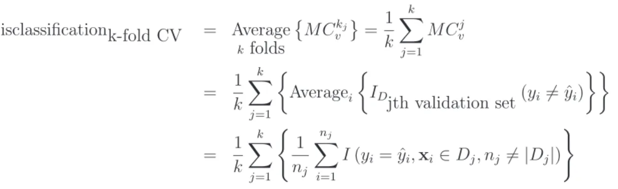
k observations, is used as the validation data set to evaluate the model. This process is repeated k times, where for each iteration a different fold is used as the validation set. The score function using k-fold cross validation is defined as
Accuracyk-fold CV = Average k folds Akj v = 1 k k X j=1 Ajv (2.5.1) = 1 k k X j=1 Averagei ID jth validation set(yi = ˆyi) = 1 k k X j=1 ( 1 nj nj X i=1 I(yi = ˆyi,xi ∈Dj, nj =|Dj|) ) where Aj
v is the accuracy calculated using thejth validation set for the classifier trained using training dataD=D/Dj, that is
Ajv = 1 nj nj X i=1 I(yi = ˆyi,xi ∈Dj, nj =|Dj|)
11 2.5. Cross Validation Misclassificationk-fold CV = Average k folds MCkj v = 1 k k X j=1 MCj v = 1 k k X j=1 Averagei ID jth validation set(yi 6= ˆyi) = 1 k k X j=1 ( 1 nj nj X i=1 I(yi = ˆyi,xi ∈Dj, nj 6=|Dj|) ) whereMCj
v is the misclassification error of the jth validation set, for the classifier trained using training dataD=D/Dj.
As an example consider performing 10-fold cross-validation. Start by randomly dividing the data setDinto 10 folds or sets of approximately equal size, denoted asD1, D2, ..., D10. Consider
this as a process with 10 iterations or steps. In iteration 1 train the classifier using training data comprised asDt={D2, D3, D4, D5, D6, D7, D8, D9, D10}. Calculate the accuracy rate,A1v, and misclassification error rate,MC1
v, using the data in foldD1 as the validation data. In iteration 2
train the classifier using training data comprised asDt={D1, D3, D4, D5, D6, D7, D8, D9, D10}.
Calculate the accuracy rate, A2
v, and misclassification error rate, MCv2, using the data in fold
D2 as the validation data. Continue the process, as shown in table 2.3 until iteration 10 is
completed. The accuracy and misclassification rates are then calculated as
Accuracy10-fold CV = 1 10 10 X j=1 Ajv Misclassificationk-fold CV = 1 10 10 X j=1 MCvj.
Table 2.3: 10-fold cross validation (iteration process).
Iteration Training data: Dt Validation Data: Dv Accuracy Misclassification 1 Dt={D2, D3, D4, D5, D6, D7, D8, D9, D10} D1 A1v M Cv1 2 Dt={D1, D3, D4, D5, D6, D7, D8, D9, D10} D2 A2v M Cv2 3 Dt={D1, D2, D4, D5, D6, D7, D8, D9, D10} D3 A3v M Cv3 .. . ... 9 Dt={D1, D2, D3, D4, D5, D6, D7, D8, D10} D9 A9v M Cv9 10 Dt={D1, D2, D3, D4, D5, D6, D7, D8, D9} D10 A10v M Cv10
2.5.2
Hold-Out Cross Validation
Hold out cross validation is a variation of the k-fold cross validation method where k = 2
the validation data Dv. A shown in table 2.4 the data set D is thus partitioned into two approximately equal sized sets, denoted as D1 and D2. In iteration 1 the first fold, D1, is used
as the training data to build the classifier while the second fold, D2, is used to validate. The
process is repeated except the data sets are swapped, that is in iteration 2 the second fold,D2,
is used to train while the first fold, D1, is used to evaluate the model. The score function for
the data set D using hold-out cross validation is defined as Accuracyhold out = 12P2j=1Aj v and Misclassificationhold out = 12P2j=1MCj
v.
Table 2.4: Hold-out cross validation.
Training data setDt =⇒ Model =⇒ Validation data setDv =⇒ Accuracy & Misclassification
D1 =⇒ First =⇒ D2 =⇒ Result: A1v,Mc1
D2 =⇒ Second =⇒ D1 =⇒ Result: A2v,Mc2
2.5.3
Leave-One-Out Cross Validation
Leave one out cross validation (LOOCV) is a special case of k-fold cross where k = n, the number of observations in the data set D. Partition the data set D into n equal folds D
n =
D1, D2, D3, ..., Dnwith one observation per fold. EachDi represents a row observation of(yi,xi) where i= 1,2,3, ..., n . The training data set contains k−1 folds or n−1observations which are used to fit the model while the validation data set, which contains only one fold namely the single observation Di, is used to evaluate the model.
As demonstrated in table 2.5, in iteration i the training data areDt = {Dj wherej 6=i} and validation data are Dv ={Dj} ={xj}. The classifier is evaluated using this single observation and hence
Ajv =I(yj = ˆyj,xi ∈Dj) MCvj =I(yj 6= ˆyj,xi ∈Dj)
The misclassification and accuracy estimate for leave one out cross validation is the average of the n estimates, that is
AccuracyLOOCV = 1 n n X j=1 Aj v = 1 n n X j=1 I(yj = ˆyj,xj ∈Dj) therefore
13 2.5. Cross Validation MisclassificationLOOCV = 1 n n X j=1 MCvj = 1 n n X j=1 I(yj 6= ˆyj,xj ∈Dj)
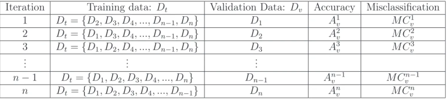
Table 2.5: Leave one out cross validation.
Iteration Training data: Dt Validation Data: Dv Accuracy Misclassification
1 Dt={D2, D3, D4, ..., Dn−1, Dn} D1 A1v MCv1 2 Dt={D1, D3, D4, ..., Dn−1, Dn} D2 A2v MCv2 3 Dt={D1, D2, D4, ..., Dn−1, Dn} D3 A3v MCv3 ... ... ... n−1 Dt ={D1, D2, D3, D4, ..., Dn} Dn−1 An−v 1 MCvn−1 n Dt ={D1, D2, D3, D4, ..., Dn−1} Dn Anv MCvn
Chapter 3
Classification Using the Naive Bayes and
Logistic Regression Classifiers
3.1
Introduction
This chapter provides an introduction to the Naive Bayes and logistic regression classifiers for binary classification. Section 3.2 discusses the basic theory of Bayes rule and section 3.3 dis-cusses the Naive Bayes classifier in detail. Section 3.4 disdis-cusses the logistic regression classifier, including discussion on how to estimate the logistic regression model parameters.
3.2
Classifiers Based on Bayes Rule
The Bayes rule classifier uses Bayes theorem to predict the new classl,l = 0,1for the observed x . It estimates the posterior probability P(Y =l |X =x) for each class l. Observations are classified to the class that has the highest probability (Zaki and Meira Jr, 2014, page 467; Gareth et al., 2013, page 38), thus the predicted class for observationx is given as
ˆ
y=argmaxl {p(Y =l|X=x)} (3.2.1) Bayes theorem can be derived from the basic probability concept by using the conditional probability rule
p(X=x, Y =l) = p(Y =l |X=x)p(X=x)
= p(X =x|Y =l)p(Y =l) (3.2.2)
equating both sides yields
p(Y =l| X=x)p(X=x) = p(X=x|Y =l)p(Y =l)
and thus
p(Y =l |X=x) = p(X=x|Y =l)p(Y =l)
p(X=x) (3.2.3)
p(X=x) is the probability of observing X=xfrom any class l, l= 0,1given as
p(X=x) = p((X=x, Y = 0)∪(X =x, Y = 1)) = p(X=x, Y = 0) +p(X=x, Y = 1)
From equation 3.2.2
p(X=x) =p(X=x|Y = 0)p(Y = 0) +p(X=x|Y = 1)p(Y = 1) (3.2.4) Substituting equation 3.2.4 into the denominator of equation 3.2.3 yields Bayes theorem which gives the posterior probability in term of the likelihood and the prior probability. p(Y = l | X = x) is posterior probability of the observation in class l given the distribution of X =x,
p(X= x|Y =l) is the likelihood function of observing X assuming Y belongs to class l and
p(Y=l)is the prior probability of class l.
p(Y =l |X=x) = p(X=x|Y =l)p(Y =l) p(X=x|Y = 0)p(Y = 0) +p(X=x|Y = 1)p(Y = 1) = 1p(X=x|Y =l)p(Y =l) X l=0 p(X=x|Y =l)p(Y =l) (3.2.5)
where p(x) is the marginal probability. Bayes rule in equation 3.2.1 can be rewritten as a posterior probability ˆ y = argmaxl {p(Y =l|X=x)} = argmaxl p(X=x|Y =l)p(Y =l) 1 X l=0 p(X=x|Y =l)p(Y =l) = argmaxl {p(X=x|Y =l)p(Y =l)}
17 3.2. Classifiers Based on Bayes Rule since the p(X =x) =
1
X
l=0
p(X = x | Y = l)p(Y = l) is fixed for a particular x. Thus the predicted class depends on the likelihood of the relevant class and prior probability of that class as follows (Zaki and Meira Jr, 2014, page 468)
ˆ
y =
argmax
l∈ {0,1} {p(X=x|Y =l)p(Y =l)}
3.2.1
Estimating the Prior Probability
The likelihood, p(X=x|Y =l), and the prior class probabilities, p(Y =l), can be estimated from the training data set D (Zaki and Meira Jr, 2014, page 468). Divide the training data set D by the number of the classes l. Let Dl represent the subset of the training data set D labeled as the class l, l = 0,1, that is
D = {XǫRp which have class label Y =l ,l = 0,1}
D0 = {XǫRp which have class label Y = 0 }
D1 = {XǫRp which have class label Y = 1 }
The training data set has n observations and each subset Dl has nl observations. The prior probability for class l can be estimated as
p(Y=l) = nl
n for l = 0,1
3.2.2
Estimating the Likelihood
The likelihood function, p(X=x|Y =l) is estimated from the joint probability of allX=x over pdimensions, that is seek
max{L(β)} = max{p(XǫRp |Y =l)}
If all the features or attributes are numeric either a parametric, for example using the multi-variate normal distribution, or a non-parametric approach can be followed (Zaki and Meira Jr, 2014, page 468). If the features or attributes are categorical then a categorical approach, using for example the multivariate Bernoulli distribution, can be utilised (Zaki and Meira Jr, 2014, page 471). Often however there is not sufficient data to reliably estimate the joint probability density or mass function, especially for high-dimensional data (Zaki and Meira Jr, 2014, page 473). An approach to over come this is to reduced the set of parameters, as described next section.
3.3
Naive Bayes Classifier
The Naive Bayes classifier is based on Bayes Rule. It assumes that the attributes, XǫRp, are conditionally independent of the response,Y (Bishop, 2006; McCallum and Nigam, 1998; Lewis, 1998). The training dataset D consists of n observations of p variables, the binary response variable denotes the class label, Y = l where l = 0,1 . The Naive Bayes classifier uses Bayes theorem directly to predict the class for a new test instance, given X = x. Applying the independent assumption of the Naive Bayes classifier, the general property of probabilities and the chain rule to equation 3.2.2 as follows:
p(X=x|Y =y) = p(XǫRp |Y =l) = p(X1 =x1, X2 =x2, ..., Xp =xp |Y =l) (3.3.1) = p(X1 =x1 |Y =l)×p(Xp−1 =xp−1, ..., Xp =xp |Y =l, X1 =x1) = p(X1 =x1 |Y =l)×...×p(Xp =xp |Y =l, X1 =x1, ..., Xp =xp) = p(X1 =x1 |Y =l)×p(X2 =x2 |Y =l)×...×p(Xp =xp |Y =l) = p Y j=1 p(Xj =xj |Y =l) (3.3.2)
We derive Naive Bayes classifier from Bayes rules by applying the equation 3.3.2 into equation 3.2.5 as follows p(Y =l |X=x) = p(Y =l) p Y j=1 p(Xj =xj |Y =l) 1 X l=0 p(Y =l) p Y j=1 p(Xj =xj |Y =l) (3.3.3)
Equation 3.3.3 is the fundamental equation for the Naive Bayes classifier. Shown above is how to calculate the probability that the response is of class l when the observed attributes have valuesx. p(Y =l)andp(Xj =xj | Y =l)are estimated from the training data set. The Naive Bayes classification rule is thus:
ˆ y = argmax l ∈ {0,1} p(Y =l) p Y j=1 p(Xj =xj |Y =l) 1 X l=0 p(Y =l) p Y j=1 p(Xj =xj |Y =l) (3.3.4)
In practice we are only interested in the numerator of equation 3.3.4, since the denominator does not depend on Y as the values of the features X are given and hence the denominator is effectively constant (Han et al., 2012, page 352). The Naive Bayes classifier is thus defined as
19 3.3. Naive Bayes Classifier follows ˆ y =largmax∈ {0,1} ( p(Y =l) p Y j=1 p(Xj =xj |Y =l) )
3.3.1
Estimating the Maximum Likelihood for Naive Bayes Classifier
We seek the maximum likelihood estimates for the Naive Bayes classifier, that is we seek estimates to maximize L(β) = p(Y =l) p Y j=1 p(Xj =xj |Y =l) (3.3.5)
From equation 3.2.2 we can rewrite equation 3.3.5 as follows
log{L(β)} = log ( p(Y =l) p Y j=1 p(XǫRp|Y =l) ) l(β) = log{p(Y =l)}+ log ( p Y j=1 p(XǫRp |Y =l) ) = log{p(Y =l)}+ p X j=1 log{p(XǫRp |Y =l)}
For the maximum likelihood estimation we seek the parameter values that maximizel(β). This leads to the following points:
• p(Y =l)≥0for all l = 0,1;
• For all Y and X, p(X =x|Y =l)≥0; • For all j = 1,2, .., p and l = 0,1 and X j,l
p(X=x|Y =l) = 1.
We utilize Lagrange multipliers to estimate the parametersp(Y =l)and p(XǫRp |Y =l)from the training data set D:
p(Y =l) = n X i=1 (Yi =l) n = count(Yi) n where i = 1,2, ..., n and l = 0,1. n X i
(Yi =l) = count(Yi) is simply the number of times that the label Yi =l is seen in the training data set.
Similarly, the maximum likelihood estimates for the p(X=x|Y =l) parameters for all l = 0,1, for alli= 1,2, ..., nand for allj = 1,2, ..., p take the following form
p(X=x|Y =l) = n X i=1 (Yi =l, Xij =xij) n X i=1 (Yi =l) = count i (XǫR p, Y =l) count(Yi =l) where count i (Y =l, X =x) = n X i=1
(Yi =l, Xij =xij)we simply count the number of times label
Y =l is seen in conjunction with xj taking valuex; count the number of times the labelY =l is seen in total; then take the ratio of these two terms.
It must be noted that the parameter estimation or learning described above is fairly general. The only special requirement is the Naive Bayes assumption which assumes conditional inde-pendence of features. This makes it a Naive Bayes classifier (Zhu, 2010).
3.4
Logistic Regression
Binary logistic regression is an approach to learning the function of the posterior probability
p(Y =l |X=x) . The aim is to determine the target variabley which is binary, yǫ(0,1). The target variable is influenced by the associated predictor variables x, x= [x1, ..., xp]′ǫRp. The predictor variables can be quantitative or qualitative (nominal or ordinal). Logistic regression models can be used to predict the probability thatybelongs to a particular class (Hastieet al., 2009, page 95).
3.4.1
The Logistic Regression Model
Logistic regression is the logit or the natural logarithm of the odds ratio (Peng and So, 2002). It models the relationship between the target variableydenote byp(Y =l|X =x), as a linear function of predictor random variables denoted by g(x)
g(x) = β′x
= β0 +β1x1+β2x2+...+βpxp
where β(p+1)×1 is a vector of the unknown parameters β = [β0, β1, β2, . . . , βp]′ and x(p+1)×1
21 3.4. Logistic Regression relationship between the probability of an observation being in class l and the linear function of g(x). The probability that y is in the class 1given the data, denoted by π1, is modeled as
π1 = p(Y = 1|g(x)) = exp(g(x)) 1 + exp(g(x)) (3.4.1) = 1 exp(−g(x))(1 + exp(g(x))) = 1
exp(−g(x)) exp(g(x)) + exp(−g(x))
= 1
1 + exp(−g(x))
The sum of the total probability is equal to one, since there are two class
p(Y = 1|g(x)) +p(Y = 0|g(x)) = 1 Therefore π0 = p(Y = 0|g(x)) = 1−p(Y = 1 |g(x) = 1− exp(g(x)) 1 + exp(g(x)) = 1 + exp(g(x))−exp(g(x)) 1 + exp(g(x)) = 1 1 + exp(g(x))
From equation 3.4.1 denote π = p(Y = 1|X=x) as the probability of observing y in class 1
given the data x. The logistic regression function of π can be expressed as
π = exp(g(x))
1 + exp(g(x)) (3.4.2)
The odds ratio is defined as the ratio of the probability of success and the probability of failure. Given π as the probability of success, the odds ratio is defined as odds= π
1−π. The odds ratio is a non-negative function, that is the odds≥0, as shown in figure 3.4.1a.
(a) Relationship between odds and probability. (b) Relationship between logit and probability. Figure 3.4.1: Odds, logit and probability
By rearranging the logistic regression function of equation 3.4.2 it can be seen that the odds ratio is an exponential function of g(x)since
π = exp(g(x)) 1 + exp(g(x)) π(1 + exp(g(x))) = exp(g(x)) π+πexp(g(x)) = exp(g(x)) π = exp(g(x))−πexp(g(x) π = exp(g(x))(1−π) π 1−π = exp(g(x)) = exp(β ′x) (3.4.3)
The logit of π is observed by taking the logarithm of both sides of the odds ratio of equation 3.4.3. The logistic regression model predicts the logit of π. π is the predicted probability that
Y = 1, from x. The logit of the probability of success, π, is a linear function of the predictor variablesxand unknown parameters β. As shown in figure 3.4.1b, if the probability of success
π = 1
2 then the logit of π is equal to zero. If the probability of success is greater than 1 2 then
the logit ofπ is positive. A probability of success less than 1
2 corresponds to the negative result
of logit of π.
In summary the logistic regression model can be formulated as:
logit(π) = ln π 1−π = g(x) = β′x = β0+β1x1+β2x2+...+βpxp
23 3.4. Logistic Regression
3.4.2
Estimation of the Logistic Regression Model Parameters
The response variable y is binary such that each Y belongs to one of the two classes 0 or 1
with fixed probability of being in each class π1 or π0 = (1−π1). The probability distribution
function of p(Y = l|X=x) is the probability of observing Y belongs to class l ∈ {0,1} given X, has a Bernoulli distribution with probability of success is π
p(Y =l|X=x) =
(
πyi
i (1−πi)1−yi for yi = 0,1
0 otherwise
where E(Yi |x) =µi =πi and V ar(Yi |x) =σi2 =π(1−πi).
Logistic regression models the number of observation in each class based on the sample obser-vations. Consider taking a random sample of size ni. Letmi denote the number of successes, thus mi is the sum of yi, mi > 0. There are ni independent Bernoulli random variables with fixed probability of successπand failure(1−π). mi has a Binomial distribution with parameter
π, sample sizeni,mi ∼binomial(ni, π):
p(Mi =mi|X =xj) = nmii
πmi(1−π)ni−mi
Note that E(Mi | x) = µi = niπ and V ar(Mi |x) = σ2i =niπ(1−π). The likelihood is given by L(π,β) = n Y i=1 ni mi πmi(1−π)ni−mi
Since log is an increasing function, the maximum log likelihood is the same as the maximum likelihood. The log converts the product into a sum, that is
ln{L(π,β)} = n X i milnπi+ (ni−mi) ln(1−π) + ln nmii (3.4.4) whereln ni mi
is a constant, independent of the unknown parameters and hence it can be ignored when the derivatives are taken with respect to the unknown parameters.
Substituting equation 3.4.2 into equation 3.4.4 yields ln{L(π,β)} = ln ( n Y i ni mi πmi(1−π)ni−mi ) l(π,β) = n X i=1 ln (πmi) + ln (1−π)ni−mi + ln ni mi = X i milnπ+ (ni−mi) ln(1−π) + ln nmii = X i milnπ−miln(1−π) +nln(1−π) + ln nmii = X i mi(lnπ−ln(1−πi)) +nln(1−π) + ln nmii = n X i=1 miln π 1−π +nln(1−π) + ln ni mi
where we assume that
ln π 1−π =g(xi) =β′xi =β0+β1x1i+β2x2i+...+βpxpi and hence l(π,β) = n X i=1 miβ′xi+n(1 + exp(β′xi)) −1 + ln ni mi ∴l(β) = n X i=1 miβ′xi−n(1 + exp(β′xi)) + ln nmii
To find the maximum likelihood, L(β) , differentiate the log likelihood with respect to the unknown parameters β and set the derivatives equal to zero. The resulting equations are known as the score equations, that is forj = 0, . . . , p
l′(β j) = ∂ln{L(β)} ∂βj = n X i=1 mixij − nixijexp(β′xi) 1 + exp(β′xi) = X i xij(mi− niexp(β′xi) 1 + exp(β′xi)) = X i xij(mi−nip(y= 1 |X=xi)) = 0
25 3.4. Logistic Regression Thus the j equations can be expressed as
l′(βj) =
n
X
i
xi(mi−niπ) for j = 0,1, ..., p
It is convenient to express these in matrix form, that is as
l′(β) = ∂l(β) ∂β =X(m−µ) (3.4.5) where X(m−µ) = x10 · · · x1p x20 · · · x2p .. . . .. · · · xn0 · · · xnp ′ m1 m2 .. . mn − µ1 µ2 .. . µn = n X i=1 xi0(mi−µi) n X i=1 xi1(mi−µi) .. . n X i=1 xip(mi−µi)
When setting these p+ 1 nonlinear equations of the p+ 1 parameters equal to zero there is no closed form solution. The nonlinear equation can be solved using the Newton Raphson algorithm, which requires the second derivatives, called the Hessian matrix
3.4.2.1 The Newton Raphson Method
The Newton Raphson method can be used to find solution for the nonlinear score equations [Hastie et al., 2009, page 99; Izenman, 2009, page 243] as follows
l′(βj) = n
X
i
There are p+ 1 equations since j = 0,1, ..., p, that is l′(β0) = n X i xi0(mi−niπi) = 0 l′(β1) = n X i xi1(mi−niπi) = 0 ... = ... l′(βp) = n X i xip(mi−niπi) = 0 These score equations are typically denoted as a vector
l′(β) = ∂ln{L(β)} ∂β0 ∂ln{L(β)} ∂β1 ... ∂ln{L(β)} ∂βp = n X i xi0(mi−niπi) n X i xi1(mi−niπi) ... n X i xip(mi−niπi) = X(m−µ)
where X, mand µare defined above.
The partial derivatives of the components of l′(β) are
l′′(βj) = ∂ ′′ln{L(β)} ∂βiβj = − n X i ni
xij(xijexp(β′x)(1 +exp(β′x))−xijexp(β′x)exp(β′′x))
(1 + exp(β′X))2 = − n X i nix′ij(
(exp(β′x) + exp(2β′x))−exp(2β′x)
(1 + exp(β′x))2 )xij = − n X i nix′ij( exp(β′x) (1 + exp(β′x)))xij = − n X i nix′ij( exp(β′x) (1 + exp(β′x))(1 + exp(β′x)))xij = − n X i nix′ijπi(1−πi)xij l′′(βj) = − n X i x′ijΣixij
The components of the covariance matrix are Σi = δ2 = n
27 3.4. Logistic Regression matrix is given by l′′(β) = ∂′′ln{L(β)} ∂βiβj ij for i, , j = 0,1,2, ..., p = ∂′′ln{L(β)} ∂β′′ 0 ∂′′ln{L(β)} ∂β′ 0β′1 · · · ∂′′ln{L(β)} ∂β′ 0βp′ ∂′′ln{L(β)} ∂β′ 1β′0 ∂′′ln{L(β)} ∂β′′ 1 · · · ∂′′ln{L(β)} ∂β′ 1βp′ ... ... . .. ... ∂′′ln{L(β)} ∂β′ pβ′0 ∂′′ln{L(β)} ∂β′ pβ′1 · · · ∂′′ln{L(β)} ∂β′′ p = − n X i x′ i0Σxi0 − n X i x′ i0Σxi1 · · · − n X i x′ i0Σxip − n X i x′ i0Σxi1 − n X i x′ i1Σxi1 · · · − n X i x′ i1Σxip .. . ... ... − n X i x′ i0Σxip − n X i x′ i1Σxip · · · − n X i x′ ipΣxip = − n X i x′ i0Σxi0 n X i x′ i0Σxi1 · · · n X i x′ i0Σxip n X i x′ i0Σxi1 n X i x′ i1Σxi1 · · · n X i x′ i1Σxip ... ... ... n X i x′ i0Σxip n X i x′ i1Σxip · · · n X i x′ ipΣxip = −X′ΣX (3.4.6)
The Newton’s Raphson iterative approach to finding maximum likelihood ML estimates is a building block for the iteratively re-weighted least squares (IRLS) algorithm.
By beginning withβ(0) = 0the(j)ststep gets substituted by the(j+ 1)thstep until the learning rate, LL′′′((ββ) is equal or close to zero.
= ˆβ(j)+ L
′(β)
[L′′(β)]
= ˆβ(j)+ [L′′(β)]−1L′(β) (3.4.7)
Keep updating equation 3.4.7 until there is a small change between the components from one iteration to the next.
matrix notation can written as ˆ β(j+1) = ˆβ(j)+ [x′Σx]−1X(m−µ) = [x′Σx]−1xΣxβˆ(j)+ [x′Σx]−1xΣΣ−1(m−µ) = [x′Σx]−1xΣ n xβˆ(j)+Σ−1(m−µ)o = [x′Σx]−1xΣz (3.4.8) where z=nxβˆ(j)+Σ−1(m−µ)o the ith is component ofz is zi =x′iβˆ (j) + yi−µi πi(1−πi)
The update equation, equation 3.4.8, is written in the generalized least squares estimator form with
• Σas the diagonal matrix consisting of weights; • z a target vector;
• X matrix data;
• βˆ is the update parameter; • µi =niπi mean of the predictor; • π is a probability of success.
ˆ
β,z and Σare updated at every step since they are dependent onβ(j). Equation 3.4.8 depends
on the assumption that x′Σx is invertible. This is acceptable when n > p+ 1. The IRLS algorithm converges in almost all pragmatic situations (Hastie et al., 2009)
3.4.3
Using Logistic Regression as a Classifier
There are two different ways to assign observation xto a class. Both methods depend on the maximum likelihood estimates. The maximum likelihood estimates the parameters β to give estimates of the logistic function as
ˆ
g(x) = βˆ′x (3.4.9)
29 3.4. Logistic Regression If g(ˆ x) ≥0 assign xi to class 1, l = 1, otherwise xi belongs to class 0, l = 0. This is typically refereed to as logistic analysis An equivalent classification procedure is to use the likelihood estimated ofg(x)ˆ in the equation 3.4.9 to estimate the posterior probability P (Y =l |X =x)
as follows ˆ p(y= 1|X=x) = exp(ˆg(x)) 1 + exp(ˆg(x)) = 1 1 + exp(−ˆg(x)) = 1 1 + exp(−βˆ′x)
x is assigned to class one, l = 1 if the posterior probability Pˆ(Y = 1 |X=x)≥c. Where c is some cutoff value. alternatively x is assigned to the class zero, l= 0 (Izenman, 2009).
Chapter 4
Classification Trees
4.1
Introduction
This chapter gives an introduction to classification trees. Section 4.2 gives a basic theory of the binary classification tree. Section 4.3 discusses the impurity function. It also states an important theorem of node impurity and tree impurity. Section 4.4 discusses the splitting rule for decision trees using the Gini index and Entropy index. It also discusses how to prune the maximum tree using cost complexity pruning and cross validation methods.
4.2
Binary Classification Trees
A classification tree is also known as a decision tree (Ross. J, 1986). A classification tree is built through a process of either splitting or not splitting each parent node in the classification tree into two internal nodes. At each node the tree algorithm searches through all the variables one by one to obtain the best split. The starting point for splitting is denoted by a root node t
at the top of the tree, see figure 4.2.1 below . The split is decided by a conditionc for a single variable x, x≤c (Breiman et al., 1984) as shown in table 4.1.
Split Class of Y Row Total
0 1
xj ≥c n11 n12 n1+
xj ≤c n21 n22 n2+
Column Total n+1 n+2 n++
Table 4.1: Classification table: The binary split ofY for variable xj.
Figure 4.2.1: A figure depicting the root node, non-terminal and terminal nodes of a classifica-tion tree.
As shown in figure 4.2.1 nodes are either root, terminal or non-terminal nodes. A non-terminal node is also called a parent or internal node and these nodes have at least one child node. A binary split is decided by a condition value c, a single variable x as follows: if x≤c then split to tL assigned to the right son node, otherwise tR assigned to the left son node. The process continues until all the variables in data set X are split. A node that does not split, that is a node that has no child, is called terminal node or a leaf node or external node. All observations in a terminal node are assigned to one class and hence a terminal node is assigned a class labels. Each tree has more than one terminal node (Breiman et al., 1984).
4.3
Impurity Functions
An impurity function is a function Φdefined on the set of all L- tuples of numbers (p1, ..., pL), where pl is a non-negative function satisfying pl > 0, where
L
X
l=0
pl = 1 with the following properties (Breiman et al., 1984, page 24):
1. Φis maximum when all the classes have equal probability, Φ 1
L, 1 L, . . . , 1 L ;
2. Φis minimum when the probability of one class is one and the remaining classes are zero,
Φ (1,0,0, ...,0),Φ (0,1,0, ...,0), ...,Φ (0,0,0, ...,1) the nodes contain only one class; 3. Φ is symmetric function of p0, p1, ..., pl gives small tree and under fitted and loose gives
over fit decision tree; if the permutation of Φremain the same then Φ (p0, p1, p2, ..., pl) =
Φ ( ¯p0,p¯1,p¯2, ...,p¯l).
4.3.1
Node Impurity
33 4.3. Impurity Functions
i(t) = Φ (p(0 |t), p(1|t), p(2 |t), ..., p(l |t))
The node impurity function is a maximum when the probability of split s is equal to pl = L1, a minimum when the probability of split s is equal to pl = 0or 1. pl = 0 the node contains only one class [Raileanu and Stoffel, 2004; Breiman et al., 1984, page 25]. The node impurity function is calculated at each step of splitting the observations in the node into two subset nodes L, R with associated probability
pL= n1+ n++ (4.3.1) and pR= n2+ n++ (4.3.2) The goodness of split s at a nodet, denoted by Φ(s, t), is defined as
△i(s, t) = Φ(s, t) =i(t)−pLi(L)−pRi(R)
The best split sof the node t is the split with largest△i(s, t) or equivalently with the smallest value ofpLi(L) +pRi(R) (Ripley, 1996; Breiman et al., 1984, page 32)
△i(s, t) =⋆ max
sǫQt
△i(s, t)
The best split at each node maximizes the decrease in impurity between the nodes △i(s, t)⋆ , which partitions the data into the left and right child or son nodes.
4.3.2
Tree Impurity
The impurity of the tree T, denoted by I(T), is calculated across the terminal nodes in the tree. The tree impurity is calculated as
I(T) = X tǫT′ I(t) = X tǫT′ p(t)i(t)
where T′ denotes the set of terminal nodes of treeT
0.
The tree impurity is a maximum only if the goodness of the split△i(s, t)is maximum (Breiman
et al., 1984). At any node t of the sub-tree Te using the split s, splits the node into tR and tL. The new sub-tree T′ has impurity function
IT˜=X
tǫT˜
I(t) +I(tR) +I(tL)
where T˜′ denotes the set of terminal nodes of sub-tree T˜.
The decrease in tree impurity is calculated by subtracting the impurity of sub-tree T˜ from the impurity of tree T
I(T)−I(T′) =I(t) +I(t
R) +I(tL)
The goodness of split based on the tree impurity is △I(s, t) = I(t) +I(tR) +I(tL) where △I(s, t) = I(t) +I(tR) +I(tL)
= i(t)p(t)−i(tR)p(t)−i(tL)p(t)
= (i(t)−i(tR)−i(tL))p(t)
= (i(t)−pRi(tR)−pLp(tL))p(t)
= △i(s, t)p(t)
The goodness of split tree impurity △I(s, t) is equal to the node impurity△i(s, t)multiplied by the estimate of the probability of node t, p(t). The same maximum split point, s⋆ , will be chosen in either impurity function (Breiman et al., 1984, page 33). A tree is grown by contractually minimizing the split impurity, and hence the tree impurity, until the stopping criterion is satisfied.
4.4
Splitting Rules
There are many criteria which can be defined for selecting the best split at each node. In the context of classification the goal is to minimize the impurity. As result we select the split that will reduce the node impurity (Breimanet al., 1984, 37). Two common node impurity functions are the Gini index and the Entropy index functions.
4.4.1
Gini Index
The Gini coefficient is a measure of statistical dispersion (Sheen and Anitha, 2012). The Gini index at node t is defined as
G(t) =i(t) = Φ (p(0 |t), p(1|t), ..., p(L|t)) = L X l6=j p(l |t)p(j |t)
35 4.4. Splitting Rules Note that for binary splits where L= 0,1
G(t) = X l6=j p(l |t)p(j |t) = 1 X l=0 p(l |t) (1−p(l |t)) = 1 X l=0 p(l |t)− L X l (p(l |t))2 = 1− 1 X l=0 (p(l|t))2
According to [Breiman et al., 1984; Therneau et al., 1997, page 103 ] there are two interpre-tations of the Gini index. In binary classification there are two classes: L = 0,1. The Gini index is measure or sum of the variance across the classes. The Gini index uses the probability
0≤ pl ≤1. If the probability is close to zero or one the Gini index gives smaller value. Small values mean that the observations in the node are from one class. The Gini index for binary variables is G(t) =i(t) = 1−p(0|t)2−p(1|t)2 = 1−(1−p(0 |t))2 +p(0 |t)2 = 1−1−2p(0|t) +p(0|t)2+p(0|t)2 = 1−1−2p(0|t) + 2p(0|t)2 = 1−1 + 2p(0 |t)−2p(0 |t)2 = 2p(0|t)−2p(0|t)2 = 2p(0|t) [1−p(0 |t)] = 2p(0|t)p(1|t)
Using the values in table 4.1, the Gini index of node t is calculated as
G(t) = 2 n+1 n++ 1− n+1 n++
The Gini index for splitting the nodet into two child nodes is given by
GSplit(t) = pLG(tL) +pRG(tR)
where pL is the proportion of cases in the node t sent to the left child node and pR is the proportion sent to the right child node. The best split is the split that has the smallest value of
goodness of split for node t and split s is defined as
△i(s, t) = Φ(s, t) = G(t)−pLG(tL)−pRG(tR)
= G(t)−GSplit(t)
The split with maximum △i(s, t)is equivalent to the split with minimum GSplit(t) (Breiman
et al., 1984, page 103). The idea of the CART method (Breiman et al., 1984) is to determine the goodness of split △i(s, t) at each split s, sǫQt, where Qt is the set of all possible splits at nodet and then to select the best split s⋆ given as
△i(s, t) =⋆ max ⋆ sǫQt (G(t)−pLG(tL)−pRG(tR)) = max ⋆ sǫQt △i(s, t)
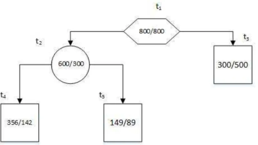
Example 3.1: Consider the binary split of the nodet1 as shown in figure 4.4.1.
Figure 4.4.1: Binary split the nodet1.
The Gini index indexG(t1)used for splitting the root nodet1and the goodness of split △i(s, t)
are calculated below.
The probability of p(0|t1) = 1 600800 and the probability of p(1|t1) = 1 600800 and hence
G(t1) = 2 800 1 600 800 1 600 = 1 2
the Gini index for the nodes t2 and t3 are calculated as
G(t2) = 2 600 900 300 900 = 0.44444 G(t3) = 2 200 700 500 700 = 0.40816
37 4.4. Splitting Rules The probability of splitting node t1 intot2 and t3 is thus
pt2 = 900 1 600 = 0.5625 pt3 = 700 1 600 = 0.4375
The Gini split of node t1 is
GSplit(t1) = pt2G(t2) +pt3G(t3)
= 0.5625×0.44444 + 0.4375×0.40816 = 0.42857
The goodness of split for Gini index at the node t1 is this
△Ginii(s, t) = G(t1)−GSplit(t1)
= 0.5−0.42857 = 0.07143
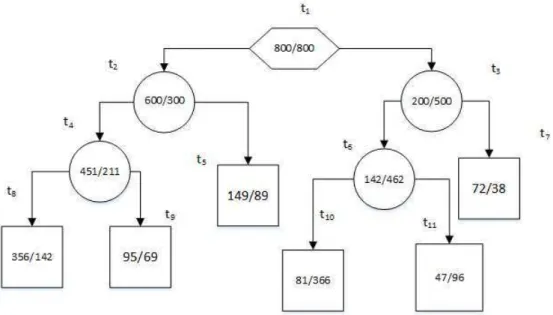
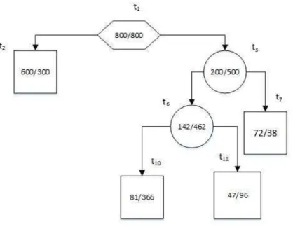
Example 3.2: Consider the example of binary tree shown in figure 4.4.2.
Figure 4.4.2: An example of a binary tree.
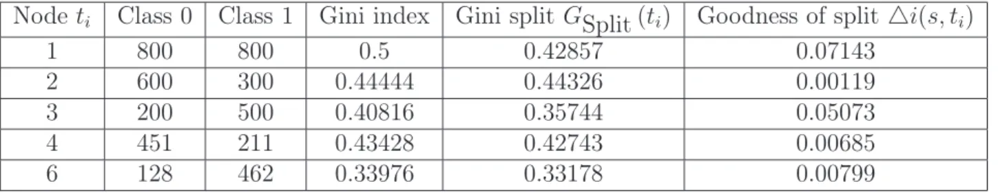
For each non-terminal node in the tree the Gini index and split△i(s, t)calculates are obtained shown in table 4.2
Table 4.2: The Gini split and goodness of the split in the non-terminal nodes in the tree depicted in figure 4.4.2.
Node ti Class 0 Class 1 Gini index Gini split GSplit(ti) Goodness of split △i(s, ti)
1 800 800 0.5 0.42857 0.07143 2 600 300 0.44444 0.44326 0.00119 3 200 500 0.40816 0.35744 0.05073 4 451 211 0.43428 0.42743 0.00685 6 128 462 0.33976 0.33178 0.00799
4.4.2
Entropy Index
The Entropy function is defined as (Breimanet al., 1984)
i(t) = Φ(p(0|t), p(1|t), ..., p(L|t)) = − L X l=0 p(l|τ) logp(l|τ)
Note that for binary splits where L= 0,1
i(t) =−p(0|t) logp(0|t)−p(1|t) logp(1|t)
Using the values in table 4.1. The entropy index of a node is calculated as
Entropy(t) =i(t) =−(n1+ n++ )llog(n1+ n++ )−(n2+ n++ ) log(n2+ n++ )
The goodness of a split based on the entropy measure is given by
△i(s, t) = Φ(s, t) =Entropy(t)−pLEntropy(tL)−pREntropy(tR)
Both the entropy and Gini indices have been used widely in the CART methodology, see for example Breiman et al. (1984); Strobl et al. (2007).
Example 3.3: Refer to figure 4.4.1. The Entropy index, Entropy(t) used for splitting the root node t1 is calculated with the goodness of split △Entropyi(s, t) . The probability of p(0|t1) =
800
1 600 and the probability of p(1|t1) = 800 1 600 Entropy(t1) = − 800 1 600 log 800 1 600 − 800 1 600 log 800 1 600 = 0.30103
39 4.5. Splitting Procedure The Entropy index for the nodes t2 and t3 are thus
Entropy(t2) = − 600 900 log 600 900 − 300 900 log 300 900 = 0.27643 Entropy(t3) = − 500 700 log 500 700 − 200 700 log 200 700 = 0.25983
The probability of splitting a node t1 intot2 and t3 is thus
pt2 = 900 1 600 = 0.5625 pt3 = 700 1 600 = 0.4375
The Entropy split of the node t1 is thus
EntropySplit(t1) = 0.5625×0.27643 + 0.4375×0.25983
= 0.26917
The goodness of this split, based on the entropy measure, at node t, is △Entropyi(s, t) = 0.301029996−0.269167974
= 0.03186
Table 4.3: The Entropy split and goodness of the split in the non-terminal nodes in the tree depicted in figure 4.4.2.
Nodeti Class 0 Class 1 Entropy index Entropy split GSplit(ti) Goodness of split △i(s, ti)
1 800 800 0.5 0.26917 0.03186 2 600 300 0.44444 0.27286 0.00057 3 200 500 0.40816 0.23544 0.02438 4 451 211 0.43428 0.26850 0.00333 6 128 462 0.33976 0.22236 0.00478
4.5
Splitting Procedure
The following procedure is used to select the splitting variable and the splitting value at the nodet (Breimanet al., 1984):
1. Determine the Gini split at node t among the child branches over all possible decision points for each variable Xj at each node;
2. Select the variable and the critical value, c, of that variable with the smallest Gini split at node t, denoted byxjc and use it for splitting;
3. Repeat this process at each node until each node has at least one observation or meets the minimum requirement of the observations at each node.
The procedure is the same for other choices of impurity function, for example the entropy impurity function.
4.5.1
Maximum Tree
The maximum tree is denoted by Tmax =T0. This tree is the result of splitting the root node
into several sub-nodes depending on the data set D and the impurity function. Splitting of nodes (internal nodes) carries on until all terminal nodes that are generated have at least one observation or all the observation belong to the same class or we declare the node to be a terminal node if satisfies the following condition
max△R(s, t)≤cR(t)
where c is a constant between 0≤ c≤1 and R(t) is the misclassification rate of node t. The result of Tmax is decreasing sequence of sub-trees where T0 is the full tree and T∞ is the tree without any splitting or terminal nodes:
T0 ≥T1 ≥T2 ≥, ...,≥T∞
To s