Online Learning with Bayesian Classification Trees

Online Learning with Bayesian Classification Trees

Samuel Rota Bul`o

FBK-irst

Trento, Italy

Peter Kontschieder

Microsoft Research

Cambridge, UK

Mapillary

Graz, Austria

Abstract

Randomized classification trees are among the most pop-ular machine learning tools and found successful applica-tions in many areas. Although this classifier was origi-nally designed as offline learning algorithm, there has been an increased interest in the last years to provide an online variant. In this paper, we propose an online learning algo-rithm for classification trees that adheres to Bayesian prin-ciples. In contrast to state-of-the-art approaches that pro-duce large forests with complex trees, we aim at construct-ing small ensembles consistconstruct-ing of shallow trees with high generalization capabilities. Experiments on benchmark ma-chine learning and body part recognition datasets show su-perior performance over state-of-the-art approaches.

1. Introduction

Random classification forests are often the preferred ma-chine learning tool due to their efficiency, scalability, and robustness. They found successful application in many areas such as computer vision [21], bio-informatics [26], medical data analysis [9], data-mining [24],etc.

Random forests are usually trained in batch (or offline) modality,i.e. all training data is expected to be given in ad-vance and once a forest is trained it cannot be updated with new, labelled samples. However, there are application do-mains where the training data is not available in advance, but is collected over time, and inference might be required at any moment. Online learning approaches can serve such purposes and have a number of advantages over batch meth-ods: they are more flexible as they can work in the presence of online data generation processes, can adapt to distribu-tions varying over time, do not need to store the training set during the learning phase, to name just a few.

Joining the online learning paradigm with classification trees is particularly difficult due to the recursive nature of this classifier. Moreover, the presence of (typically) deter-ministic split decisions within the tree complicates using new data samples to correct decisions that were taken at an

earlier level. Consequently, the number of works address-ing online learnaddress-ing within decision trees in the literature is rather small and we review the most related ones next. The Hoeffding tree algorithm [11] maintains a set of candidate splits in the leaves and tracks their quality as new data ar-rives. The Hoeffding bound is used to control the amount of data that should be collected before a probably-optimal split selection can be ensured. In [20] a similar idea is pur-sued, but the leaf splitting condition changes and an online bagging [19] strategy is adopted. A modification over [20] was presented in [23], which uses reservoir sampling to keep track of a fixed-length, unbiased set of training sam-ples for updating the trees. The work in [2] also extends the Hoeffding tree algorithm by introducing an adaptive-size version, allowing to mix differently-adaptive-sized trees. Their approach imposes restrictions on the number of split nodes such that shallower trees can adapt more quickly to changes in the distribution of the incoming data stream while deeper trees adapt more slowly and therefore maintain a longer-term memory. The work in [10] also maintains sets of can-didate splits in the leaf nodes. There, the authors provide a decision forest construction algorithm, which dynamically partitions the data into structure and estimation samples, the former being used to influence the tree structure and the lat-ter being used to estimate the leaf predictions. The work of [13] presents an alternative approach by governing the tree growing phase by a Mondrian process. There, label distributions are kept at each node and controlled by a hier-archy of normalized, stable processes.

A remaining limitation of state-of-the-art online algo-rithms for random forests is a tendency to producing over-sized trees, as the split selection process is unaware of the tree complexity and split functions are very simple. More-over, trees tend to overfit, thus requiring large forests to achieve good performance, which however implies slow-down of the inference process and increased memory re-quirements. In particular, the algorithms that keep candi-date splits in the leaves during training suffer from a pro-hibitive memory cost as trees get deep [10] or require mul-tiple passes over the training data [10, 20].

Contributions. In this paper, we introduce a novel on-line learning algorithm for Bayesian classification trees that tries to overcome the aforementioned limitations, by tak-ing a different perspective. Our goal is to learn tree clas-sifiers with a shallow structure and high generalization ca-pability. We trade shallow tree structures for more com-plex split decision functions that jointly take into account multiple feature dimensions and their correlations. Our on-line learning procedure is a Bayesian approach that itera-tively replaces a posterior distribution over trees, obtained after observing a new training sample, with a simpler, para-metric distribution. This surrogate posterior is determined within the parametric family in a way to fit the updated pos-terior distribution with the minimum loss of information. Our algorithm is characterized by update rules for the tree hyper-parameters that are free from cumbersome learning rate selection and allow us to naturally absorb the informa-tion carried by each new sample. Due to the Bayesian learn-ing principle, which takes the uncertainty about the tree’s parameters into account, we can obtain tree classifiers that do not overfit. In summary, the proposed method matches our initial intention of obtaining ensembles containing few, shallow and well-generalizing trees. The provided experi-mental evaluation confirms our model choice and its ben-efits are shown with quantitative experiments on standard benchmark machine learning and more complex body part recognition datasets.

Relationship to Bayesian tree models. Bayesian models for decision trees have appeared in the literature for offline learning – namely the Bayesian hierarchical mixture of ex-perts (BHMEs) [3], Bayesian CART models [5, 6, 8, 25], Bayesian BART models [7] – and for the online learning modality with dynamic tree models [22, 1]. Our model differentiates from these approaches since we are propos-ing a parametric, Bayesian model for decision trees that is trained in an online fashion, i.e. we update over time a posterior distribution over the space of decision trees, whereas other similar approaches like BHMEs (despite sharing structural similarities) work in an offline fashion and consider sigmoid-gated hierarchical mixture of experts in the underlying model hypothesis space.

2. Classification Trees

In this section we recap classification trees to provide all the necessary notation and definitions that are subsequently used for introducing our Bayesian online learning approach. Consider a classification problem with input spaceXand a finite set of categorical labelsY. Aclassification treeis a classifier consisting of decision nodes and prediction nodes, arranged into a tree-structure. Decision nodes correspond to the tree’s internal nodesN and are responsible for routing data samples to an appropriate prediction node (i.e. leaf) in

L. Each decision noden∈ N takes a routing decision for a data samplex∈ Xvia arouting functionbn:X → {0,1}. Ifbn(x) = 1, thenxis routed to the left sub-tree, otherwise it goes to the right one. Akin to conventional decision trees, we consider binary decision functions of the following type:

bn(x) =1θ⊤

nξn(x)≥0, (1)

where1P is an indicator function for the truth value ofP. The decision functionbndepends on a node-specific feature mapξn : X →R

d_n

, and ad_{n-dimensional parameter}

vec-torθn ∈ R

d_n

(see also [15]). Starting from the root node and after visiting a number of decision nodes,xends up in a prediction node, where the actual class assignment takes place. Indeed, each prediction nodeℓ ∈ Lholds a proba-bility distributionπℓ= (πℓy)y∈Y over labels inYthat will be used to deliver the final prediction for the data sample reaching it.

A classification tree, denoted by t, is identified by its structure S and its parameters, i.e. t = (θ,π, S), where

θ = {θn}n∈N holds the parameters of all decision nodes and π = {πℓ}ℓ∈L contains the class distributions of all prediction nodes. The structure of the tree comprises the set of nodesN, leavesLand their relations. Moreover, it includes the node-specific feature mapsξn.

Given a tree t = (θ,π, S), the predictive distribution

p(y|t;x)for data samplexis defined as

p(y|t;x) =X

ℓ∈L

r(ℓ|t;x)πℓy, (2)

whereπℓydenotes the probability of a sample ending in leaf

ℓto take on class y, andr(ℓ|x)is regarded as therouting function, which is1for the leafℓwhere samplexis actually routed to, and0elsewhere.

To give an explicit form to the routing function, we intro-duce the following binary relations that depend on the tree structure: ℓ ւ nis true ifℓbelongs to the left subtree of noden, andnցℓis true ifℓbelongs to the right subtree of

n. By exploiting these relations we can factorize the routing function as

r(ℓ|t;x) = Y

n∈N

bn(x)1ℓւn(1−bn(x))1nցℓ. (3)

Although the product in (3) runs over all nodes, only the decision nodes along the path from the root node to the leaf

ℓare affected.1

3. Bayesian Online Classification Trees

In this section we present our novel online learning al-gorithm for classification trees, adhering to Bayesian prin-ciples. Our approach falls within the theoretical framework

1

1ℓւn and1nցℓare both zero for allnnot being ancestors ofℓ.

ofBayesian Online Learning(BOL) [18], also known as as-sumed density filteringin the control literature [14], and is related toexpectation propagation[17].

3.1. Overview

LetDi = {(x1, y1), . . . ,(xi, yi)} ⊂ X × Y denote a collection ofilabelled examples, and assume to have a prior distributionp(t)defined over the set of decision trees. In standard Bayesian inference it is possible to compute the posterior distribution oftgiven the collection of data points

Diby recursively employing the Bayes rule in the following way:

p(t;Di)∝p(yi|t;xi)p(t;Di−1), (4) wherep(t;D0) = p(t). This formula captures the change in the posterior distribution due to an added training sample

(xi, yi), when the posterior distribution afteri−1samples is treated as the new prior for the incoming data point.

Although the rule in (4) seems to be structurally suitable for an online scenario, it cannot instantly be used for online learning, because in general it requires knowledge about the

entiretraining set. However, if we could store the posterior from the previous(i−1)samples, and compute the normal-izing constant, we would obtain an online learning approach by repeatedly applying (4), without the need of revisiting past samples. The BOL framework implements this idea by recursively building asurrogatedistribution for thetrue

posteriorp(t;Di). The surrogate distribution is confined to a pre-defined, parametric family of distributionsQ, which can be compactly stored. In the rest of the paper we will denote byq(t;hi), or more compactlyqi(t), the surrogate distribution of the true posterior of t giveni samples, hi being the parametrization of the distribution.

The recursive construction of this surrogate distribution alternates a Bayes update step, integrating information con-veyed by new training data akin to (4), with a projection step, which re-maps the obtained distribution in the para-metric familyQ.

Update step. Let qi_{(t)be the surrogate posterior} distri-bution oftfromisamples, which is taken as prior for the update step of a new data sample (xi+1, yi+1). By appli-cation of the Bayes rule we obtain the following updated posterior distribution:

ˆ

qi+1_(t)∝p(y

i+1|t;xi+1)qi(t). (5) The familyQ, whereqi _{belongs to, is typically selected in} a way to make the computation of (5) tractable. This prop-erty however is not necessarily preserved by the distribution

ˆ

qi+1_{in case we use it for a subsequent update. For this}

rea-son, a projection step is required.

Projection step. The projection step finds the best ap-proximation ofqˆi+1 _{within the parametric familyQ, in a}

way to minimize the loss of information. In this regard, the sought distributionqi+1 _{∈ Qis the one that minimizes the}

following Kullback-Leibler (KL) divergence:

qi+1∈arg min

q∈Q DKL qˆ i+1_kq

. (6)

After performing the projection, qi+1 _{can be regarded as}

a surrogate of the true posterior distributionp(t;Di+1)of

t giveni+ 1samples, which can be used as a new prior distribution for subsequent updates (see, Fig. 1).

Inference. At any time, we can use the current surrogate posterior distribution, say qi_(t)

, to compute the posterior predictive distributionfor a new data samplex. The poste-rior predictive distribution, denoted byp(y;x, hi), provides the expected class distribution that we obtain forxwith a decision treetsampled from the surrogate posterior distri-butionqi_:

p(y;hi,x) =Eqi[p(y|t;x)] (7)

whereEqi[·]denotes expectation with respect toqi. In the

rest of the paper we will refer to (7) as the posterior predic-tive distribution for convenience, but the reader should keep in mind that it is actually an approximation of thetrue pos-terior predictive distributionp(y;x,Di)that one obtains in standard (offline) Bayesian inference from the observed set of labelled samplesDi. Indeed, we replace the true poste-riorp(t;Di)with the surrogate posteriorqi(t), which has been sequentially estimated fromDias previously detailed.

3.2. Surrogate Posterior for Classification Trees

The key component of the online learning algorithm de-scribed above is the surrogate posterior. On one hand, we

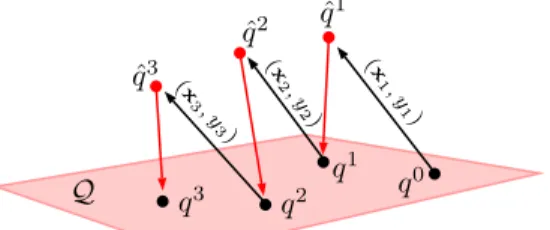
b b b b Q q0 b b b q1 q2 q3 ˆ q1 ˆ q2 ˆ q3 (x 1 , y 1₎ (_x 2 , y 2₎ (_x 3 , y 3₎

Figure 1. Example of the Bayesian online learning process: we start with a prior distributionq0(t)over the set of decision trees, and apply the update rule in (5) to incorporate the information from the first sample (x1, y1). The obtained posteriorqˆ

1

(t) is then reprojected in the parametric family of distributionsQ us-ing (6). The resultus-ing distributionq1

(t)is a surrogate distribution of the true posteriorp(t;D1), which can be used as a new prior for the next update step. We keep iterating this process as new training samples arrive. At any moment, the most recent surrogate posteriorqi

would like to keep it simple such that the projection step in (6) and the computation of the posterior predictive distribu-tion in (7) remain tractable. On the other hand, we would like to have it complex and multi-modal to best possibly capture the true posterior distribution. The solution we pro-pose is a compromise between these two contradicting re-quirements.

Unimodal with fixed structure. Assume in first place to have a pre-defined tree structureSˆ. The surrogate posterior over treest= (θ,π, S)can be defined as a factorization of independent distributions over the tree’s parameters, which takes the following parametric form:

q(t;h) =δˆS(S) Y n∈N qn(θn;Σn,µn) Y ℓ∈L qℓ(πℓ;αℓ). (8)

The first term in (8) is a Dirac measure that supports only trees with structureSˆ. Each decision function’s parame-terθn follows a multivariate Gaussian with meanµn and covarianceΣ_{n, i.e.qn} ∼ Gauss_(µn,Σ_{n), while each} pre-diction node’s class distributionπℓfollows a Dirichlet dis-tribution with parameterαℓ,i.e.qℓ∼Dir(αℓ)(see Fig. 2). The argumenth= ( ˆS,Σ_{,µ,α)ofqholds all the parameters} of the distribution (a.k.a.hyperparameters of the tree).

The distribution in (8) is unimodal for most parametriza-tions and, under this modelling choice, the projection step in (6) turns into the following, independent minimizations over the different parameters ofqi _{(see, Subsection A.1 of} the supplementary material):

(Σi_n+1_,µi_n+1₎∈_{arg min} Σ,µ Eqˆ i+1[−logq_n(θ_n;Σ,µ)], (9) αi_ℓ+1∈arg min α Eqˆ i+1[−logq_ℓ(π_ℓ;α)], (10)

where the expectations are with respect to the updated pos-teriorqˆi+1_{. Moreover, the structure of the tree is preserved}

by the update in (6),i.e.Sˆi+1 _{= ˆS}i_{. In Sec. 4, we describe}

how to solve (9) and (10).

Multi-modal. A simple way to better capture the true pos-terior distribution consists in modeling the surrogate

poste-θn∼Gauss(µn,Σn)

πℓ∼Dir(αℓ)

Figure 2. The parameters of the tree are given byθnfor each de-cision nodenandπℓfor each prediction nodeℓ. Each decision node’s parameterθnis a multivariate Gaussian with meanµnand covarianceΣn. Each prediction node’s parameterπℓis a Dirichlet-variate with concentration vectorαℓ.

rior as a uniform mixture of distributions

q(t;h1, . . . , hm) = 1 m m X j=1 q(t;hj), (11)

where q(t;hj_{) is defined as in (8). In such a way, each}

of the mixture components might consider a different tree structure (including possibly different feature mapsξn per

node). Accordingly, the tree structures are still assumed to be given, but multiple structures can now be integrated into a single, multi-modal distribution. The projection step in (6) for the multi-modal posterior can be approximated by independent projections of each single surrogate poste-rior forming the mixture in (11) (see, Subsection A.2 in the supplementary material). Finally, the posterior predictive distribution under the multi-modal posterior has the simple closed-form p(y;h1i, . . . , h m i ,x) = 1 m m X j=1 p(y;hj_i,x), (12)

where hj_i is the parameter of the surrogate posterior dis-tribution oft obtained fromisamples for thejth mixture component in (11). Please note that in (12), we average the posterior predictive distribution overm _{online-trained}

Bayesian trees, as known from conventional forests [4, 9]. Next, we will focus on algorithmic details (e.g. parameter updates, implementation notes,etc.) of individual trees.

4. Algorithmic Details

In this section we provide further details about the form of the posterior predictive distribution in (7) as well as the update formulae for the surrogate posterior’s parameters, providing the solutions for (9) and (10). Due to a lack of space we omit the full derivations and a detailed discussion about the computational complexity of our model, which are however available in the supplementary material. Posterior predictive distribution. The posterior predic-tive distributionp(y;hi,x)as given in (7) can be computed

in closed-form as follows: p(y;hi,x) = X ℓ∈L αi ℓy |αi_ℓ|1 ρ(ℓ;hi,x). (13)

This distribution is the counterpart of (2), which we obtain by marginalizing out the tree using the surrogate posterior distributionq(t;hi). The first term in the summation is the

expectation ofπℓyunder the Dirichlet distribution with

pa-rameterαiℓ, where| · |1is theℓ1norm. The second term is

a stochastic routing function, which takes the form:

ρ(ℓ;hi,x) = Y

n∈N

whereβi

n(x)represents the following probability of sample xto be routed to the left child at nodenin a random treet

distributed asq(t;hi):

βni(x) = Φ(µin⊤ξ˜ni(x)).

Function Φ is the cumulative distribution function of the standard normal distribution, and ξ˜i

n is a Σin-normalized

version of the node-specific feature mapξn, given by ˜ ξin(x) =ξn(x) h ξn(x)⊤Σinξn(x) i−1/2 . (15) Inuitively,βi

nrepresent a softening of the hard decision rule bn in (1), induced by the uncertainty about the decision

node’s parametrization.

Remark 1 Function(14)is still valid if we replaceℓwith any other nodemin the tree, and in that caseρ(m;hi,x) provides the probability of reaching node m. We will use this later in this section. Moreover, we will also use a variant of the posterior predictive distribution, denoted by p(y|m;hi,x), which conditions on a nodem of the tree. This provides the posterior predictive distribution if we took mas the starting node for the prediction.

Update rule for µ and Σ_{. The update rules forµ and} Σ_{can be obtained by solving the cross-entropy} minimiza-tion problem in (9). Since the Gaussian distribution is in the exponential family, we can determine a solution to the aforementioned minimization problem by moment-matching. The resulting update rules are given by

µi_n+1=µi_n+κnΣinξ˜ni , (16) Σi+1 n =Σin− κ2n+κnµin⊤ξ˜ni (Σi nξ˜ni) Σi nξ˜ni ⊤ , (17) where we wroteξ˜i

nas a shortcut forξ˜ni(xi+1)and κn =φ

µi_n⊤ξ˜ni

(unL −unR)an, (18)

whereφ(·)is the probability density function of the stan-dard normal distribution, nL and nR denote the left and

right child of node n, respectively, an = _p(ρ_y(_in₊₁;h_;i_h,x_i,xi+1_i+1)₎,

andun=p(yi+1|n;hi,xi+1).

Remark 2 (Scale invariance) The posterior predictive distribution will not change if we scale each mean µin by cn and each covarianceΣin by cn2 for any cn > 0 (e.g. cn = 1/kµink2). Moreover, the update rules in(16)and

(17)are consistent under the same transformation,i.e. we obtaincnµin+1 andc2nΣni+1 if we transformµin and Σin in the same way. Hence, we can safely scaleµi_n+1 andΣi+1

n in this sense after each update round, without affecting the outcome of the algorithm. This helps to avoid numerical instabilities.

Update rule forα. The update rule forαcan be deter-mined by solving (10). Sinceπℓfollows a Dirichlet

distri-bution with parameterαℓ, we obtain the following

moment-matching equations:

Eqi+1

ℓ [log(πℓ)] =Eqˆ

i+1[log(π_ℓ)]. (19)

With some manipulations of the two expectation terms, we end up with the following system of equalities forz∈ Y:

ψ(αi_ℓz+1)−ψ(|αi_ℓ+1|) =ψ(αiℓz)−ψ(|αiℓ|) + aℓ(1z=yi+1−uℓ) |αi ℓ|1 (20)

where aℓ and uℓ are defined as in (18), and ψ(·) is the

digamma function. We solve the system using Newton-Raphson iterations, where few iterations (typically 5–10) are necessary to achieve a good accuracy. This provides us with a solution to (10) as required. We refer to [16] for the derivation of the fixed-point iterations.

Prior distribution. We select a prior distribution from the same familyQas the surrogate posterior given in (8) and it is identified by the timestamp i = 0, i.e.p(t) = q0(t). We instantiate a prior distribution by providing a tree struc-tureSˆ0_{with some pre-defined depth and with randomized}

feature map functions ξn in each node having the form, ξn(x) = [Pnx; 1], where Pn is a projection matrix and 1 accounts for a bias term. The prior terms for the deci-sion nodes’ parameters are improper, flat priors with mean

µ0=0_andΣ0_{→ ∞}I_{, which induces the following update} once the first sample is observed:µ1n=ξn(x1)/kξn(x1)k2

andΣ1

n = I/κ2n−µn1µ1n⊤, where κn is computed as per

(18) with ξ˜0

n = 0. The prior parameters for the

predic-tion nodes are uniformly sampled in the range (0, ǫ], i.e.

0 < α0

ℓy ≤ ǫ, where0 < ǫ ≪ 1is a small, non-negative

constant, with the exception of having one peaked prefer-ence per class uniformly distributed across the leaves. Implementation notes The update of the surrogate tree posterior distribution after having seen a new training sam-ple (xi+1, yi+1)can be carried out by traversing the tree

twice. The first traversal is top-down and computesρn = ρ(n|hi,xi+1) for each node n, which is required in the

definition ofκn, in (18) and in (20). This is done by

ini-tializing ρ⊤ = 1, where ⊤ ∈ N is the root node, and by computing for each decision node n ∈ N visited in breadth-first orderρnL =β

i

n(xi+1)ρnandρnR=ρn−ρnL,

wherenL andnR are the left and right child of noden. It

is then possible to run over the leavesℓ ∈ Lto compute

uℓ =αiℓyi+1

|αi_ℓ|1and finally obtain the posterior

predic-tive probabilityp(yi+1;hi,xi+1) = Pℓ∈Lρℓuℓ. We have

Algorithm 1Online learning of Bayesian classification tree Require: (xi+1, yi+1): next training sample

Require: hi: latest surrogate posterior parameter (ifi >0)

Require: Sˆ0_{: a tree structure (ifi= 0)} 1: ifi= 0then

2: initializeα0,µ0andΣ0_{(see,Prior distribution)}

⊲Forward pass over tree computesρn=ρ(n|hi,xi+1) 3: ρ⊤ ←1

4: for alln∈ N in top-down, breadth-first orderdo

5: ρnL ←β i n(xi+1)ρn ⊲ nL: left child ofn 6: ρnR ←ρn−ρnL ⊲ nR: right child ofn 7: uℓ← αi ℓyi+1 |αi ℓ|1 ,∀ℓ∈ L 8: p(yi+1;hi,xi+1)←P_ℓ∈Lρℓuℓ 9: computeαi_ℓ+1by solving (20),∀ℓ∈ L

⊲Backward pass over tree:un=p(yi+1|n;hi,xi+1) 10: for allnin bottom-up, breadth-first orderdo

11: un←unR+ (unL−unR)β i n(xi+1) 12: computeκnas per (18)

13: ifi= 0then ⊲Prior initialization

14: µ1n← ξn(xi+1) kξn(xi+1)k2 15: Σ1 n ←I/κ2n−µ1nµ1n⊤ 16: else 17: computeµin+1as per (16) 18: computeΣi+1 n as per (17)

19: rescaleµin+1andΣin+1as per Remark 2

returnhi+1: new surrogate posterior parameters

prediction nodeℓby solving the system (20). The second traversal is bottom-up and computes the updates for the de-cision nodes’ hyperparameters. We run again over the nodes

n∈ N, but in bottom-up, breadth-first order. Once a node

nis visited, we computeun =unR+ (unL−unR)β i n(xi+1)

andκnas per (18). Finally, we calculateΣin+1andµin+1

us-ing (16) and (17), since all the required quantities are avail-able. A summary is provided in Alg. 1.

Fast, single path inference During inference, exact com-putation of the posterior predictive distribution requires traversing the tree entirely. The complexity is thus

O(|N |d2_{), where} d _{is the maximum decision node}

fea-ture dimensionality. However, since the routing function of each tree gets peaked on a single path after a reason-able number of samples (i ≫ 0) have been observed, we can obtain a good approximation of the posterior predic-tive distribution by taking at each decision node nthe di-rection where the samplexhas the highest probability to be routed to,i.e. left ifβni(x)>0.5, and right otherwise. This

decision can be taken efficiently by evaluating the sign of

µin⊤ξn(x), because βni(x) > 0.5 ⇐⇒ µin⊤ξn(x) > 0.

With this trick, we reduce the per-tree complexity during inference toO(d_{log2|N |), which is the same as for offline,}

oblique decision trees [12, 15]. Please note, thatlog2|N |is

much smaller for our compact trees than for typically deeper oblique decision trees.

5. Experiments

We assess several variants of our algorithm on differ-ent datasets, including standard machine learning (ML) classification benchmarks (Sec. 5.1) and pixel-wise se-mantic labelling of Kinect [21] data (Sec. 5.2). For all experiments, we provide baseline results of state-of-the-art online random forest approaches, using their pub-licly available reference implementations. We validate our learner against Mondrian Forests (MF) [13], Online Ran-dom Forests (ORF) [20], and Consistent Online Forests (COF) [10] (the latter code includes a re-implementation of ORF). As additional baselines, we provide results for offline random forests (RF) [4] and offline oblique random forests (obRF) [15]. Please note however, that offline forest results are not directly comparable to online results, as their train-ing expects theentiredataset to be given in advance. We fix

ǫ = 0.01(see last section), which may serve as guideline for other datasets (we did not experience large sensitivity when varying it). For each dataset we train at most 8 trees for our method (no reasonable improvement was found with more) and we allow only asingle epoch over the datafor our trees to properly simulate an online scenario unless ex-plicitly stated otherwise. Instead, all forest competitors (of-fline and online) comprised 100 trees with up to 15 epochs over the data (specifically recommended for [20, 10]).

5.1. Classification performance on ML datasets

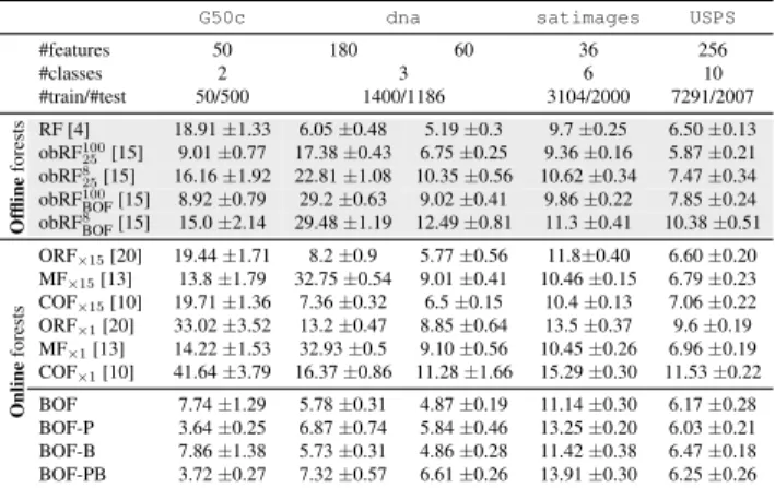
We tested onG50c,dna,satimagesandUSPSsince they were also (partially) selected in [10, 13], and cover dif-ferent granularity of difficulty with respect to dataset char-acteristics (#feature dimensions, #classes, #train/#test sam-ples). A summary is provided on top of Tab. 1, followed by blocks for offline ([4, 15], grayed block) and online for-est results, respectively. All reported scores are average classification errors with standard deviations in [%] (from 10 repetitions or cross-validation folds for standard parti-tioning of datasets),i.e., lower is better. Offline forest re-sults should mainly demonstrate the effects due to different complexities of decision node functions: For instance, [4] uses randomly selected, single feature channels (i.e. axis-aligned splits) while [15] applies more complex, oriented hyperplanes, thus incorporating a larger feature space. On-line forest results for ORF, MF and COF could be approx-imately reproduced with default parameter settings in their code (or suggested in their papers), which we also used for training/testing on datasets not evaluated in their papers.

We dub our method as Bayesian Online Forest2_{(BOF) in}

2_{While knowing that we introduced an ensemble of Bayesian trees}

rather than a Bayesian forest, we use the term forest as we average akin to conventional forests

G50c dna satimages USPS #features 50 180 60 36 256 #classes 2 3 6 10 #train/#test 50/500 1400/1186 3104/2000 7291/2007 Offline forests RF [4] 18.91±1.33 6.05±0.48 5.19±0.3 9.7±0.25 6.50±0.13 obRF100 25 [15] 9.01±0.77 17.38±0.43 6.75±0.25 9.36±0.16 5.87±0.21 obRF8 25[15] 16.16±1.92 22.81±1.08 10.35±0.56 10.62±0.34 7.47±0.34 obRF100 BOF[15] 8.92±0.79 29.2±0.63 9.02±0.41 9.86±0.22 7.85±0.24 obRF8 BOF[15] 15.0±2.14 29.48±1.19 12.49±0.81 11.3±0.41 10.38±0.51 Online forests ORF×15[20] 19.44±1.71 8.2±0.9 5.77±0.56 11.8±0.40 6.60±0.20 MF×15[13] 13.8±1.79 32.75±0.54 9.01±0.41 10.46±0.15 6.79±0.23 COF×15[10] 19.71±1.36 7.36±0.32 6.5±0.15 10.4±0.13 7.06±0.22 ORF×1[20] 33.02±3.52 13.2±0.47 8.85±0.64 13.5±0.37 9.6±0.19 MF×1[13] 14.22±1.53 32.93±0.5 9.10±0.56 10.45±0.26 6.96±0.19 COF×1[10] 41.64±3.79 16.37±0.86 11.28±1.66 15.29±0.30 11.53±0.22 BOF 7.74±1.29 5.78±0.31 4.87±0.19 11.14±0.30 6.17±0.28 BOF-P 3.64±0.25 6.87±0.74 5.84±0.46 13.25±0.20 6.03±0.21 BOF-B 7.86±1.38 5.73±0.31 4.86±0.28 11.42±0.38 6.47±0.18 BOF-PB 3.72±0.27 7.32±0.57 6.61±0.26 13.91±0.30 6.25±0.26

Table 1. Mean classification errors with standard deviations in[%] over 10 runs. Grayed block: Offline forest variants. Middle block: Online forest competitors. Bottom block: Proposed Bayesian On-line forest variants. See Sec. 5.1 for description.

case no projection is performed,i.e. P_{n =}I_{, BOF-P when} we perform a randomly selected projection, BOF-B when using bagging (i.e. a tree discards a sample with probability

τ), and BOF-BP when bagging and random projection are applied. All methods were trained on the same splits into training/testing. As a rule of thumb, we define a dataset-specific set of possible tree depths from where the actual tree depth is randomly selected. Specifically, we sample the tree depth from{⌈log2(|Y|)⌉, . . . ,⌈log2(|Y|)⌉+2}such

that there are at least as many leaves as number of classes.

E.g., thesatimagesdataset has 6 classes which means that we randomly select a tree depth between 3 and 5. This max tree depth is also applied for some oblique forest con-figurations, indicated by the super- and subscripts. For in-stance, obRF8_BOF means that 8 trees with the same max depth as our Bayesian trees were grown, while obRF10025

means that 100 trees with max depth 25 were trained. We obtain scores that are similar or better than all online methods we compare to, considering their 15-epoch results ORF×15, MF×15, COF×15. For thednadataset we

eval-uate with two different feature space sizes like [13]. MF seems to struggle with highdimensional inputs (see er-ror values of≈33% vs.≈9%), whereas pre-selection of in-formative dimensions yields≈1% in accuracy gain for our approach. On thesatimagesdataset we perform similar (or slightly worse) than our competitors. Finally, we also list single-epoch results for ORF×1, MF×1 and COF×1,

which, except for MF, show drastic performance reductions, inhibiting online learning without additional samples.

To illustrate the ensemble effect, we obtain the follow-ing classification errors (in [%]) when usfollow-ing (1,4,8) BOF trees. G50c: (8.1, 7.9, 7.7). dna(180): (6.1, 5.9, 5.8).

dna(60): (5.5, 5.0, 4.9).satimages: (13.0, 11.3, 11.1).

USPS: (8.3, 6.5, 6.2). Since our trees are Bayesian, they exhibit less variance than standard trees. We thus require

Training data size

102 103 104 Accuracy [%] 75 80 85 90

95 USPS Forest Accuracy

Offline RF COF [Denil et al.] ORF [Saffari et al.] MF [Lakshm. et al.] Ours

Figure 3. Sequential data arrival experiments for USPS dataset (see last paragraph in Sec. 5.1), showing test data classification accura-cies as function of seen training samples.

smaller ensembles to achieve similar/better accuracy. For different variants of our method we experience only mi-nor performance drop when applying bagging (τ = 0.3), which however linearly reduces training times. We obtain both, improvement of classification error and reduction in training time forG50candUSPSwhen applying randomly chosen projections to lower-dimensional feature spaces (by applying projection matricesP_{n). As target feature} projec-tion dimensionality we choose values approximately around

d_/2,i.e.P_n∈Rd/2×d_{. We provide a table with detailed} in-formation on Matlab timings in the supplementary material (Sec. C.1), corresponding to the experiments in Tab. 1.

Sequential data arrival performance onUSPS _{In Fig. 3}

we show the results when training and testing our tree en-semble from sequentially arriving data of theUSPSdataset, akin to the experiment in [10]. The curves show the per-formance on the test dataset as a function of the number of training samples presented to the algorithms. As can be seen, our algorithm initially performs comparably with the other methods but begins to even surpass re-trained offline forests [4] after seeing more than 500 training samples. The numbers for our method are averaged over 10 runs and again each sample was presented only once while [10, 20] allowed 15 epochs in their training protocol.

5.2. Kinect dataset

In this experiment we perform the task of pixel-wise semantic labelling (body part recognition, see Fig. 5), us-ing synthetically generated depth input images. We used the publicly available3_{dataset of [10], which provides}

pre-defined splits into training and test images, as well as the specific order and training sample center locations pre-sented to the learners. The training set contains 2000 im-ages (i.e. poses with 19 body part classes + 1 background

Training data size 104 106 Accuracy [%] 15 25 35 45 55 65 75

85 Kinect Forest Accuracy

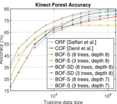
ORF [Saffari et al.] COF [Denil et al.] BOF-S (8 trees, depth 8) BOF-S (3 trees, depth 8) BOF-SD (8 trees, depth 8) BOF-SD (3 trees, depth 8) BOF-S (8 trees, depth 7) BOF-S (3 trees, depth 7)

Figure 4. Sequential data arrival experiments for Kinect dataset (see Sec. 5.2), showing test data classification accuracies as func-tion of seen training samples.

class label) from where≈50 samples per body part and im-age were collected, resulting in roughly 2 million training samples. Testing was conducted on all foreground pixels of the 500 images in the test set. Since the exact order and locations of training samples are given, we can provide a direct comparison to the baseline scores reported for [20] and [10]. Both trained forests of 25 trees, [20] was limited to depth 8 for memory reasons (to keep memory consump-tion<10GB) while [10] reports no restriction on their max-imum depth. Moreover, [10] reports that their trees were allowed to evaluate 2000 candidate offsets with 10 candi-date split node tests at a memory consumption of 1.6GB, when limiting their approach to 1000 active leaf nodes.

We trained again ensembles comprising 8 balanced Bayesian trees, using maximum depths of 7 or 8 (yield-ing 127/255 split nodes and 128/256 leaf nodes per tree, respectively). Instead of granting access to 2000 candi-date offsets, we used d _{= 100 randomly chosen}

off-sets (+1 bias dimension) per split node (dubbed BOF-S), which we sampled from a log-polar space with maximum distance of ≈35 pixels, akin to [10]. In such a way, the total number of parameters per tree for our approach is |N | ·((d_{+ 1)}2_{+ (d+ 1) +d) + 2|N | · |Y|}

(requiring

1012perΣ_n,101perµ

n,100for subspace selection viaPn

and 20 perαℓ), resulting in≈5/10MB per tree (depth 7/8).

When using only axis-aligned, diagonal covariance matri-cesΣ_{n (denoted as BOF-SD), the model memory} require-ment reduces to≈160/320kB per tree. Once only inference

Figure 5. Color-coded, qualitative examples of Kinect semantic la-belling experiment (ground truth vs. obtained result), see Sec. 5.2.

has to be performed, memory consumption can be reduced to≈110/220kB (for both, BOF-S and BOF-SD) when using the fast, single-path routing described in Sec. 4..

The plot in Fig. 4 shows the pixel labelling accuracy (percentage of correctly labelled foreground pixels of test set as in [10]) as a function of presented training data. We outperform both baselines by a significant margin over the entire sweep of training samples when using 8 BOF-S trees. For instance, after 500k training samples we improve by ≈6/8% over [10] and ≈11/13% over [20] (depth 7/8). Conversely, we approximately match the final performance of [10] at 2M samples with our depth 8 ensemble after see-ing only 20k (i.e.1/100th) training samples. Also, we only need 3 of our trees in order to reach comparable final per-formance to [10], which we illustrate with dashed lines in the plot. With our faster 8 tree training variant BOF-SD (ie.diagonalΣ_{n, shown in cyan), we approximately match} the performance of the full covariance version at the maxi-mum number of training samples. Finally, note that all re-sults for our approaches were obtained by performing the fast, single-path inference described at the end of Sec. 4. More experimental insights in the supplementary material include i) details on timings in Sec. C.1, ii) plots and dis-cussions of an increasing ensemble size for both, depth 7 and depth 8 BOF-S ensembles in Sec. C.2, iii) a guide on how to perform model selection based on the online devel-opment of the ensemble training loss in Sec. C.3.

6. Summary and Future Work

In this paper we have proposed a novel approach for on-line learning of classification trees, driven by ideas from Bayesian online learning theory. Our solution departs from state-of-the-art approaches by trying to build tree ensembles that consist of only few and compact trees with good gen-eralization capability. We achieved this goal by adopting a Bayesian learning procedure that iteratively refines a pos-terior distribution within a pre-defined parametric family in a way to best incorporate information carried by new data samples. The experimental evaluation has shown that our approach is able to perform on par or better than state-of-the-art online forest algorithms on a variety of classification tasks, while using smaller models.

We plan to extend our approach to regression, by replac-ing the prediction model in the leaves and derive proper up-date formulæ for the related parameters. We also plan to investigate a semi-parametric, Bayesian setting in order to let the tree structure be driven by the data.

Acknowledgments. This research has received funding from the European Unions Horizon 2020 research and in-novation programme under grant agreement No 687757.

References

[1] C. Anagnostopoulos and R. B. Gramacy. Dynamic trees for streaming and massive data contexts. ArXiv preprint arXiv:1201.5568, 2012.

[2] A. Bifet, G. Holmes, B. Pfahringer, R. Kirkby, and R. Gavald`a. New ensemble methods for evolving data streams. InProceedings of the 15th ACM SIGKDD Interna-tional Conference on Knowledge Discovery and Data Min-ing, KDD ’09, pages 139–148, New York, NY, USA, 2009. ACM.

[3] C. M. Bishop and M. Svens´en. Bayesian hierarchical mix-tures of experts. InProc. of Conference on Uncertainty in Artificial Intelligence, page 5764, 2003.

[4] L. Breiman. Random forests. Machine Learning, 45(1):5– 32, 2001.

[5] W. Buntine. Learning classification trees. Stat. Comput., 2:63–73, 1992.

[6] H. Chipman, E. I. George, and R. E. McCulloch. Bayesian cart model search.J. Am. Stat. Assoc., pages 935–948, 1998. [7] H. Chipman, E. I. George, and R. E. McCulloch. BART: Bayesian additive regression trees. The Annals of Applied Statistics, 4(1):266–298, 2010.

[8] H. Chipman and R. E. McCulloch. Hierarchical priors for Bayesian cart shrinkage.Stat. Comput., 10(1):17–24, 2000. [9] A. Criminisi and J. Shotton. Decision Forests in Computer

Vision and Medical Image Analysis. Springer, 2013. [10] M. Denil, D. Matheson, and N. de Freitas. Consistency of

online random forests. In(ICML), 2013.

[11] P. Domingos and G. Hulten. Mining high-speed data streams. InInt. Conf. on Knowl. Discov. and Data Mining, pages 71– 80, 2000.

[12] D. Heath, S. Kasif, and S. Salzberg. Induction of oblique decision trees. Journal of Artificial Intelligence Research, 2(2):1–32, 1993.

[13] B. Lakshminarayanan, D. Roy, and Y. W. Teh. Mondrian forests: Efficient online random forests. InAdvances in Neu-ral Inform. Process. Syst., 2014.

[14] P. S. Maybeck. Stochastic models, estimation and control. Academic Press, 1982.

[15] B. H. Menze, B. M. Kelm, D. N. Splitthoff, U. Koethe, and F. A. Hamprecht. On oblique random forests. InMachine Learning and Knowledge Discovery in Databases, volume 6912. Springer, 2011.

[16] T. P. Minka. Estimating a dirichlet distribution. Unpublished, 2000.

[17] T. P. Minka. Expectation propagation for approximate bayesian inference. InProceedings of the 17th Conference in Uncertainty in Artificial Intelligence, UAI ’01, pages 362– 369, 2001.

[18] M. Opper. A bayesian approach to on-line learning. In D. Saad, editor,On-line Learning in Neural Networks, pages 363–378. Cambridge University Press, 1998.

[19] N. Oza and S. Russel. Online bagging and boosting. InProc. of Artificial Intell. and Statistics, pages 105–112, 2001. [20] A. Saffari, C. Leistner, J. Santner, M. Godec, and H. Bischof.

On-line random forests. InIEEE - ICCV Workshop on On-line Learning for Computer Vision, 2009.

[21] J. Shotton, R. Girshick, A. Fitzgibbon, T. Sharp, M. Cook, M. Finocchio, R. Moore, P. Kohli, A. Criminisi, A. Kipman, and A. Blake. Efficient human pose estimation from single depth images.(PAMI), 2013.

[22] M. Taddy, R. B. Gramacy, and N. G. Polson. Dynamic trees for learning and design. J. Am. Stat. Assoc., 106(493):109– 123, 2011.

[23] J. Valentin, V. Vineet, M.-M. Cheng, D. Kim, J. Shotton, P. Kohli, M. Nießner, A. Criminisi, S. Izadi, and P. Torr. Se-manticpaint: Interactive 3d labeling and learning at your fin-ger tips.ACM Transactions on Graphics, 2015.

[24] A. Verikas, A. Gelzinis, and M. Bacauskiene. Mining data with random forests: A survey and results of new tests. Pat-tern Recognition (PR), 44(2):330 – 349, 2011.

[25] Y. Wu, H. Tjelmeland, and M. West. Bayesian CART: Prior specification and posterior simulation. J. Comput. Graph. Stat, 16(1):44–66, 2007.

[26] P. Yang, Y. Hwa Yang, B. B. Zhou, and A. Y. Zomaya. A re-view of ensemble methods in bioinformatics.Current Bioin-formatics, 5(4):296–308, 2010.