Bayesian Inference for Sparse Generalized
Linear Models
Matthias Seeger, Sebastian Gerwinn, and Matthias Bethge Max Planck Institute for Biological Cybernetics
Spemannstr. 38, T¨ubingen, Germany
Abstract. We present a framework for efficient, accurate approximate Bayesian inference in generalized linear models (GLMs), based on the ex-pectation propagation (EP) technique. The parameters can be endowed with a factorizing prior distribution, encoding properties such as sparsity or non-negativity. The central role of posterior log-concavity in Bayesian GLMs is emphasized and related to stability issues in EP. In particular, we use our technique to infer the parameters of a point process model for neuronal spiking data from multiple electrodes, demonstrating sig-nificantly superior predictive performance when a sparsity assumption is enforced via a Laplace prior distribution.
1
Introduction
The framework ofgeneralized linear models(GLM) [5] is a cornerstone of modern Statistics, offering unified estimation and prediction methods for a large num-ber of models frequently used in Machine Learning. In a Bayesian generalized linear model (B-GLM), assumptions about the model parameters (sparsity, non-negativity, etc) are encoded in a prior distribution. For example, it is common to use an overparameterized model with many features together with a sparsity prior. Only such features relevant for describing the data will end up having significant weight under the Bayesian posterior. Importantly, for the models of interest in this paper, inference does not require combinatorial computational efforts, but can be done even with a large number of parameters.
Exact Bayesian inference is not analytically tractable in most B-GLMs. In this paper, we show how to employ the expectation propagation (EP) technique for approximate inference in GLMs with factorizing prior distributions. We focus on models with log-concave (therefore unimodal) posterior, for which a careful EP implementation is numerically robust and tends to convergence rapidly to an accurate posterior approximation. The code used in our experiments will be made publicly available.
We apply our technique to a point process model for neuronal spiking data from multiple electrodes. Here, each neuron is assumed to receive causal input from an external stimulus and the spike history, represented by features in a GLM. In the presence of high-dimensional stimuli (such as images), with many neurons recorded at a reasonable time resolution, we end up with a lot of features,
but we can assume that the system can be described by a much smaller number of parameters. This calls for a sparsity prior, and we are able to confirm the importance of this prior assumption through our experiments, where our model achieves much better predictive performance with a Laplace sparsity prior than with a (traditionally favoured) Gaussian prior, especially for small to moderate sample sizes. Our model is inspired by [10], who identify commonly used spiking models as log-concave GLMs, but the Bayesian treatment as well as the usage of sparsity in this context is novel.
The structure of the paper is as follows. In Section 2, we introduce and motivate the model class of B-GLMs. In Section 3, we show how the expectation propagation method can be applied to B-GLMs, motivating the central role of log-concavity in this context. Our multi-neuron spiking model is presented in Section 4, and experimental results are presented in Section 5. We close with a discussion in Section 6.
2
Bayesian Generalized Linear Models
The models we are interested in here are specified in terms of primary parameters
w (or weights) and hyperparametersθ. IfDdenotes the set of observations, the likelihood isP(D|w), and the (Bayesian) prior distribution isP(w). We require that
P(w|D)∝Y
j
φj(uj), uj=wTψj, (1)
whereP(w|D)∝P(D|w)P(w) is the (Bayesian) posterior.ujis a scalar-valued1 linear function of w, and the sitesφj(·) are non-negative scalar functions. We require that all φj are log-concave, i.e. each −logφj is convex2. The role of log-concavity is clarified shortly, see also Section 3. Note that our framework can be extended with no additional difficulties to models with an additional joint Gaussian factorN(w|µ0,Σ0) in (1). Here,Σ0need not be diagonal. Most
Gaussian process models fall in our class, for example [9].
Perhaps the simplest B-GLM is thelinearone, where the likelihood is Gaus-sian and given by factorsφj(uj) =N(yj|uj, σ2), describing dataD={(ψ
j, yj)}, yj ∈R. Equivalently, yj =ψTjw+εj, whereεj ∼N(0, σ2) is noise. If the lin-ear model is used with a Gaussian prior onw, Bayesian inference can be done analytically, essentially by solving the normal equations. However, this conve-nient conjugate choice does not encode any strong assumptions about w and can severely underperform in situations where such assumptions are reasonable. What non-Gaussian priors can we use within our model class? We restrict our-selves to factorizing priors:P(w) =Q
kP(wk). Log-concave choices include the
Laplace (or double exponential) P(wk) ∝ e−ρk|wk| (sparsity); positive Gaus-sian P(wk)∝ N(wk|0, σ2k)I{wk>0} (non-negativity); or exponentialdistribution
1 Our framework applies just as well if theu
jare low-dimensional vectors, but this is not in the scope of this paper.
2
P(wk)∝e−ρkwkI{wk>0} (sparsity and non-negativity). Furthermore, any
prod-uct of log-concave functions is log-concave again.
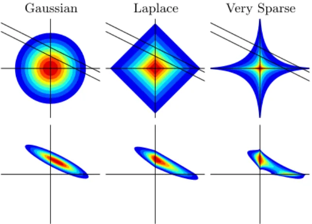
Gaussian Laplace Very Sparse
Fig. 1.Different prior distributions over coefficients ofw.
In this paper, we are principally interested in theLaplace distribution as a sparsity prior. The linear model with this prior is the basis of the Lasso [19], extensively used in Machine Learning (under names such asL1 regularization,
basis pursuit, and others). In the Lasso, we compute point estimates for the pa-rameters, by maximizing the sum of the log likelihood and the log of the Laplace sparsity prior. The latter L1 regularizer tends to force coefficient estimates to
zero exactly if they are not required.L1 penalization can be applied to
nonlin-ear GLMs as well, resulting in a convex estimation problem, for which several algorithms have been proposed in Machine Learning.
The Bayesian inference approach is quite different. Rather than just esti-mating a single parameter value, a posterior distribution over parameters is computed. More than a point estimate, we obtain credibility regions and infor-mation about parameter correlations from the posterior. Parameters are never forced exactly to zero under the posterior, since such a conclusion could not be justified from finite observations. The function of the Laplace sparsity prior in Bayesian inference is motivated in Figure 1. It leads to shrinkage of poste-rior mass towards coordinate axes (vertical in the figure), something a Gaussian prior does not do. On the other hand, the posterior remains log-concave, so that all contours enclose convex sets. The stronger sparsity prior ∝e−|aij|0.4 is not
log-concave and induces a multimodal posterior, which can be very hard to ap-proximate. Note that the role of the Laplace prior in our work here is not to provide feature selection or sparse estimation, but rather to improve our infer-ence for an overparameterized model from limited data. Note that the method proposed here has been applied to Bayesian inference for the sparselinearmodel
underlying the Lasso in [16]. However, our application here requires a nonlinear model, since the data are event times rather than real-valued responses.
Generalized linear models [5] extend the linear model to a range of different tasks beyond real-valued regression estimation, while maintaining desirable prop-erties such as identifiability, efficient estimation, and simple asymptotics. All log-concave GLMs are of the form (1). The likelihood has exponential family form, in thatP(D|w) = exp(φ(D)Tg−l(g)−a(D)), whereg =g(w) are the natural pa-rameters, andl(g) is the log partition function, which is convex ing. Ifg is linear inw, thenP(D|w) is log-concave inw, since−logP(D|w) =−φ(D)Tw+l(g) up to a constant. Therefore, any log-concave factorizing prior on w induces a B-GLM. If g(w) is composed of a linear map and a nonlinear link function, log-concavity must be established separately. A concrete example of a B-GLM of this kind is given in Section 4.
Importantly, the posteriors of B-GLMs are log-concave inw, therefore uni-modal. This property is quite crucial to ensure that our approximate inference3
method is accurate and can be implemented in a numerically stable manner. Note that many models of general interest are not B-GLMs, such as mixture models, models with Student-t likelihoods. Many of the commonly used spar-sity priors, such as “spike-and-slab” (mixture of narrow and wide Gaussian), Student-t, or∝ exp(−ρ|wk|α), α < 1 (see Figure 1 for α = 0.4), are not log-concave, and accurate approximate inference is in general a very hard problem. Furthermore, most approximate inference methods known today are numerically unstable when applied to such models.
Several approximate inference methods for B-GLMs have been proposed. The MCMC technique of [11] could be applied, together with adaptive rejection sam-pling [3] for the likelihood factors. Our approach is significantly faster and more robust than MCMC (where convergence is very hard to assess). Sparse Bayesian Learning (SBL) [20] is the most well-known method for the sparselinearmodel. SBL is related to our EP variant in [16]. It has been combined with EP and applied to B-GLMs in [12]. The main technical difference to our proposal is that they use separate techniques to deal with likelihood sites (EP, moment match-ing) and prior sites (scale mixture decomposition of Student-t), while we employ EP for all sites. The EP update for Laplace prior sites is numerically challenging, and an equivalent direct EP variant for a non-log-concave Student-t prior (used in SBL) is likely to behave non-robustly (Malte Kuss, pers. comm.). The scale mixture treatment circumvents these numerical difficulties, and stronger spar-sity Student-tpriors can be used. On the other hand, our direct approach runs significantly faster on models of interest here, where there are many more like-lihood than prior factors. The method of [12] is a double-loop algorithm, where EP is run to convergence on the likelihood sites after each update of the (prior) scale mixture parameters. Our method is also more transparent, not mixing two
3 Faced with non-log-concave models with multimodal posteriors, most approximate
inference techniques somewhat break down, with the exception of MCMC techniques, which however typically become very inefficient in such situations.
different approximate inference principles4. Finally, their method approximates
a multimodal posterior with a single Gaussian in a variational lower-bound fash-ion (SBL can be interpreted in a variatfash-ional way, see [22]), which is often quite loose. Typical robustness and “symmetry-breaking” problems in such methods are hidden in the optimization over the scale mixture (prior) parameters, which may be hard to solve properly. Even if their SBL approach is applied to a model with Laplace priors (by using the scale mixture decomposition of the Laplace, see [11]), the implications of posterior log-concavity for their method are less clear.
Note that the Laplace approximation frequently used for approximate Bayesian inference cannot be applied directly to the sparse GLM, since the Hessian does not exist at the posterior mode. A double-loop method can be derived by apply-ing the Laplace approximation to the likelihood only, this has been proposed in [20].
3
Expectation Propagation
Exact Bayesian inference is not analytically tractable for the application con-sidered here, or for most B-GLMs in general. However, it can be approximated, and our approach is based on theexpectation propagation(EP) method [7, 9]. EP results in a Gaussian approximation Q(w) to a posteriorP(w|D) of the form (1). While the latter is not Gaussian, its log-concavity (and unimodality) moti-vates such an approximation. EP is used for a linear model (Gaussian likelihood) with Laplace prior in [16], and has been used for a range of models with Gaus-sian prior and log-concave likelihood [9], albeit not for point process data (as is done here; an application to discrete-state continuous-time Markov processes was given in [8]). In general, there has not been much work on approximate inference for nonlinear models with sparsity priors (an exception is [12]).
The posteriorP(w|D) in (1) is formally a product ofJ sitesφj, normalized to integrate to one. Each siteφjis either part of the likelihoodP(D|w) or of the priorP(w). Let K be the number of variables: w ∈RK. We use a factorizing Laplace prior on w, P(w) = K Y k=1 φk(wk), φk(wk)∝e−ρ|wk|, ρ >0, (2)
whose sparsity-enducing role has been motivated above. The likelihood sites φj, j =K+ 1, . . . , J in (1) are log-concave and will be specified further below for the model of interest.
4 These principles may in fact be based on qualitatively different divergence measures,
noting that SBL has variational mean-field character [22], which uses a different di-vergence than EP [6]. Since these didi-vergences focus on different aspects of approx-imation [6], mixing them is non-transparent and may lead to algorithmic problems such as slow convergence.
The EP posterior approximation of (1) has the form Q(w) ∝ Q
jφ˜j(uj), where ˜φj(uj) = exp(bjuj−12πju2j) aresite approximationsof Gaussian form, the bj, πj are called site parameters. The log-concavity of the model implies that allπj ≥0. Some of them may be 0, as long asQ(w) is a (normalizable) Gaus-sian throughout. An EP update at j consists of computing the Gaussiancavity distribution Q\j ∝Qφ˜−1
j and the non-Gaussian tilted distribution Pˆ ∝Q\jφj, then updatingbj, πj such that the newQ0has the same mean and covariance as
ˆ
P (moment matching). This is iterated in some random ordering over the sites until convergence.
LetQ(w) =N(w|h,Σ). An EP update at sitejleads to a rank-one update ofΣ, featuringvj=Σ ψj, and costsO(K
2). Details are given in the appendix.
It is shown in [15] that for log-concave sites this update can always be done, and results inπj≥0. In this case, EP updates can typically be done in a stable way, and empirically the method converges reliably and quickly. In contrast to this, EP tends to be very problematic to run on non-log-concave models. Full updates may not always be possible (for example resulting in negative variances), and damping techniques are typically required to attain convergence at all. Cases of EP divergence for multimodal posteriors have been reported [7]. EP updates often become inherently unstable operations in these cases5.
A good initialization ofb,π depends on the concrete B-GLM. For our sparse spiking model (see Section 4), we start withb=0, andπj = 0 for all likelihood sites, but πk =ρ2/2 for prior sites, ensuring thatφk (2) and ˜φk have the same
first and second moments initially,k= 1, . . . , K.
It is reported in [16] that in the presence of a factorizing Laplace prior, EP can behave extremely unstably if w is only weakly constrained by the likeli-hood. This happens in strongly underdetermined linear models (more variables than observations), but will typically not be the case in parametric B-GLMs. For example, in our spiking model application, we have many more likelihood sites thanw components. In such cases, an initial EP update sweep over all like-lihood sites is recommended, before any Laplace prior sites are updated. In an underdetermined case, the measures developed in [16] may have to be applied.
The marginal likelihoodP(D|θ) is the probability of the data, given model and hyperparametersθ, where primary parametersw have been integrated out. It is the normalization constant in (1). This quantity, also known as partition function or evidence, can be used to conduct Bayesian tests (via Bayes factors), or to adjustθin a way robust to overfitting. EP comes with a marginal likelihood approximation, which in our case can be derived from [16, 15], together with its gradient w.r.t. θ. Details will be described in a longer version of this paper.
5
In this case, a multimodal posterior is approximated by a unimodal Gaussian, so that spontaneous “symmetry breaking” does occur. The outcome may then depend significantly on artificial choices such as site ordering for the updates, or numerical roundoff errors during the updates.
4
Sparse Feature Neuronal Spiking Model
An important approach to understanding neural systems is to build models in order to predict spike responses to natural stimuli [2]. Traditionally, single cell responses are characterized using spike-triggered averaging techniques6, allowing
for efficient estimation of thelinear receptive field, a concise description of what the cell is most sensitive to. For example, a neuron in the early visual cortex may act as a detector of certain features such as edges or lighting/texture gradients of particular orientation in a small area of the visual field: its receptive field can be thought of as a localized, oriented filter, and only the appearance of the specific event will elicit a strong response. This notion can be grounded in a spe-cific GLM: the linear-nonlinear cascade model [10]. Recent developments apply this formalism to multi-neuron responses [4, 10]. We present another important conceptual extension: rather than computing point estimates of model param-eters only, we employ a full Bayesian inference scheme, allowing us to encode desirable properties via the prior. The resulting posterior gives quantitative an-swers about localization and dispersion of inferred model parameters, together with credibility intervals (“error bars”) describing the range of uncertainty in the parameters. Assessing uncertainty is essential in this application, since neu-ral response models come with many parameters, and only a limited amount of data is available.
We adoptlinear-nonlinear-Poisson(LNP) cascade models [17], where spikes Di = {tj,i} of neuron i come from an inhomogeneous Poisson process, whose instantaneous firing rate λi(t) is a nonlinear function of the output of a linear filter. The filter coefficients are the primary parameterswi.λi(t) depends on both stimulus events as well as the spiking history of all neurons. There are stimulus-neurondependencies (normally described by thelinear receptive field) as well as
neuron-neurondependencies:λi(t) may depend on spikes fromD=∪iDi, lying in [0, t). In summary, LNP models are obtained asλi(t) = λi(wTiψ(t)), where
ψ(t) does not depend on primary parameters: a linear filter is followed by a non-linear transfer functionλi, which feeds into an inhomogeneous Poisson process. According to general point process theory [18], the negative log likelihood for spike dataDis X i − X j
logλi(wTiψ(tj,i)) + Z
λi(wTi ψ(t))dt
.
It has been shown in [10] that the likelihood is log-concave inwiifλi(·) is convex and log-concave.
The model we consider here is a generalization of a Poisson Network [13], and a special LNP model. For a sequence ofchangepoints 0 = ˜t0 <˜t1<· · ·<˜tj < . . ., we assume that ψ(t) is constant in each [˜tj−1,˜tj), attaining the value ψj there. The semantics of changepoints are given below, here we note that all spikes
6
Statistics are obtained by averaging over a window [ti−∆, ti),tia spike, character-izing effects which precede a spike emission [14].
(from all neurons) are changepoints, with ξj,i = 1 iff ˜tj ∈Di andξj,i = 0 oth-erwise. Under this assumption, the likelihood isP(D|{wi}) =QiLi(wi), where eachLi(wi) has the form (1), withφj,i(uj,i) =λi(uj,i)ξj,iexp(−τjλi(uj,i)), τj= ˜
tj−tj˜−1. Importantly, while we require that all rates λi(t) are piecewise con-stant, we do not restrict ourselves to a uniform quantization of the time axis. The changepoint spacing is far from uniform, but rather tracks current spiking activity and stimulus quantization.
A simple transfer function is λi(u) = eu, giving rise to a log-linear point process model. Another option isλi(u) =euI
{u<0}+ (1 +u)I{u≥0}, which grows linearly only [4]. The class of admissableλi is characterized in [10].
The piecewise constant featuresψ(t) encode spike history and input stimulus (with some history as well) by using windows back in time. In order to infer the precise timing of relationships, we need a narrow spacing, and thus end up with many features, only a small part of which will be necessary to describe the data. This notion is embodied in the Laplace sparsity prior. We useP({wi}) = Q
iP(wi), each factor having the form (2). The posterior for our sparse multi-neuron spiking model factorizes w.r.t. wi, each factor constituting a B-GLM of the form (1). The prior sites have the form φk,i(uk,i) = ρi
2 exp(−ρi|uk,i|)
with ψk =δk = (I{l=k})l. EP is used for approximate inference, as detailed in Section 3. It can be run in parallel across neurons, although the feature vectors
ψj are shared among them.
We describe the composition ofψ(t) informally only. A more formal descrip-tion will be given in a longer version of this paper. The spike-history part of
ψ(t) depends on windowsIl(t) = (t−∆Hl , t−∆ H
l−1], 0 =∆
H
0 < ∆H1 < . . .,
com-ponents areni,l(t) =|{j|tj,i∈Il(t)}|. These give rise to changepointstj,i+∆l for all j, i, and l ≥0. The input stimulus x(t) is a step function, changing at tI
j, j ≥1. This adds componentsx(t−∆Il) to ψ(t) for another system of lags 0 ≤∆I
0 < ∆I1 < . . .. The corresponding changepoints are tIj +∆Il for all j, l. The list of changepoints can be computed from the dataset, it does not depend on parameter settings. We also use a constant feature inψ(t), whose parameter controls the mean firing rate.
For fixed parameterswi, we can easily compute the log likelihood for some data by an accumulation of logφj,i. Here, the list of changepoints can be grown sequentially. The posterior expected log likelihood can be approximated by av-eraging over a sample drawn fromQ({wi}), or by just plugging in the posterior means. We can also sample data exactly from the model for fixed parameters
wi, using a simple variant of the Gillespie algorithm (e.g., [21]). This is possible only because we restrict ourselves to piecewise constant featuresψ(t). Sampling from the model is useful to approximate predictive probabilities for essentially arbitrary queries.
5
Experimental Results
In this section we present results for the multi-neuron spiking model of Section 4, applied to data recorded from retinal ganglion cells stimulated with white noise in
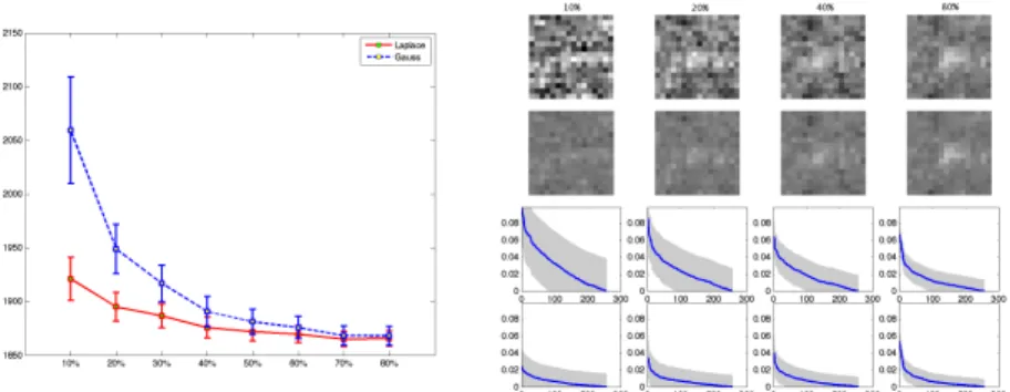
Fig. 2. Left: Comparison between Gaussian and Laplace prior for the reduced model. Hyperparameters are chosen by crossvalidation (see text). The negative log-likelihood value on the test dataset is plotted as a function of dataset size of the training set. Errorbars are obtained by sampling from the approximative posterior distribution and correspond to 2 standard deviations. Right: Receptive fields (shown are posterior means) under model with Gaussian (upper) and with Laplace prior (lower), for different training set sizes. Curves below show marginal posteriors (absolute value of mean, one std. dev. error bars, cut off at zero), decreasing order.
a whole-mount preparation. More precisely, the stimulus has been generated from an m-sequence, yielding 16x16 bitmaps of spatially and temporally decorrelated light intensity patterns presented at about 50 Hz (20 ms between stimulus onset and offset). We selected four out of 27 neurons for our analysis, with average mean firing rate of 9 Hz for a recording time of 658 s . Details about the recording technique and the spike-sorting method can be found in [23].
The goal of our first analysisis to investigate how the Gaussian and the Laplace priors differentially affect the inference in our neuronal spiking model, depending on the amount of data used. This study is carried out for one out of the four neurons, with a substantially reduced set of parameters, in that we use a single time lag ∆I
0 = 120 ms for stimulus dependence, six windows
∆Hl = 0,1,10,20,40,80,160 ms for spike history, and a constant offset feature. The complete data set was partitioned into test set, validation set (10% each), and a training pool (80%). The training sets are selected as increasing portions of the latter, in steps of 10%. Our B-GLM at present comes with a single hyper-parameterρ, the scale of the prior. This parameter is determined, independently for the Gaussian and the Laplace variant, by maximizing the log likelihood of the validation set under the posterior mean parameters for a training set of size 10%.
The log likelihood scores on the test set (Figure 2, left) show that the Laplace prior configuration of our model clearly outperforms the Gaussian prior variant. As expected, the difference is most pronounced for small training set sizes, and does eventually vanish for large data sets, when the prior has less and less in-fluence on the inference. This confirms the statistical validity of the sparseness assumption for this task. As discussed in Section 2 and Figure 1, the Gaussian
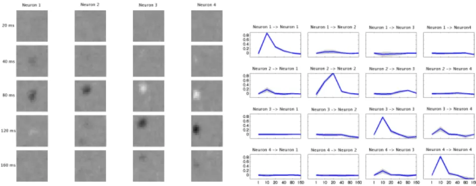
Fig. 3. Left: Stimulus dependence for the four neurons (columns) at different time lags (rows). Shown are posterior means. Gray scale from dark (minimum) to light (maximum). Right: Causal dependencies between the four neurons. Each plot shows the parameter value as function of increasing time lag. Shown are posterior mean and three std. dev. Note that all inter-dependency parameter estimates are positive, while the offset parameters for each of the neurons is significantly negative. Self-excitation can be clearly seen, explaining the bursting behaviour seen in the data.
has a strong tendency to push large values towards zero, while the Laplace prior concentrates more on shrinking smaller values strongly to zero (see Figure 2, right; 80%, lower panel). The intolerance of even a small number of large coeffi-cients means that the prior variance of the Gaussian has to be chosen larger than for the Laplace, leading to very diffuse receptive field estimates (see Figure 2, right).
The goal of our second studyis to demonstrate that the sparse Bayesian estimation framework allows us to obtain reliable results also for more complex models with a large number of parameters. We did the same experiments as above with a full setup consisting of n = 4 neurons, five time lags for stimu-lus dependency (20,40,80,120,160 ms), the same six windows for spike history and constant offset feature as above, resulting in a total number of parameters K = 1305 (versus K = 263 for the restricted setup). We use training set size 10%, and score Gaussian and Laplace variant by the negative test set log like-lihood for the one neuron used in the restricted setup. We have nlh1,Gauss =
1953.14, nlh1,Laplace= 1920.35, diff1,Gauss−Laplace= 32.79 for the restricted, and
nlh4,Gauss = 2984.5, nlh4,Laplace = 1992.59, diff4,Gauss−Laplace = 991.91 for the
full setup. Both Gaussian and Laplace variant become worse on the full setup, owing to the fact that there is a much larger number of parameters and inter-dependence features, explaining the same number of spikes (although the data from the other neurons can be used as well in the full setup). In summary the Laplace prior becomes more import the more parameters the model has.
Using the full training pool (80%, 178326 changepoints), we obtain reliable posterior mean estimates for both thestimulus-neuron and the neuron-neuron
receptive fields (Figure 3, left) are localized in space and time, as is typical for retinal ganglion cells. Self-feedback dominates the spike history parameters (Figure 3, right), allowing the model to explain short burst behaviour of retinal cells [1].
6
Conclusion
We have presented a method for approximate Bayesian inference in generalized linear models with factorizing priors, which is accurate, efficient, and numerically robust. In particular, we applied this method to a multi-neuron spiking model and showed that the usage of a Laplace sparsity prior leads to superior prediction performance at no extra cost, compared to the standard Gaussian choice.
Our method is versatile and flexible, catering to various applications as the family of B-GLMs is large, containing the sparse linear model, the generalized linear and Gaussian process models for classification, robust regression, ordinal regression, survival analysis and many more. While these models are often fitted to data by point estimation techniques, our framework can be used to obtain a good approximation to the full posterior distribution efficiently.
In future work, we will explore ideas to speed up our method drastically, for example by exploiting the fact thatψj+1−ψj is sparse. We will also consider factor representations of the parameterswi, for example to learn wide-horizon, fine-grained spatio-temporal receptive fields, and extensions of our basic model by latent variables. Both will render the complete model non-log-concave, but our method here will still be useful as subroutine in a surrounding belief propagation architecture.
Acknowledgments
We thank G. Zeck for providing us with data, and J. Macke for helpful discus-sions. Supported in part by the IST Programme of the European Community, under the PASCAL Network of Excellence, IST-2002-506778.
Appendix
EP update: match moments of ˆP(uj)∝φj(uj) ˜φj(uj)−1Q(uj) andQ0(uj), so bj →b0j =bj+∆bj, πj →π0j =πj+∆πj. IfQ(w) =N(h,Σ), thenQ0(w)∝ exp((∆bj)uj − 1 2(∆πj)u 2 j)Q(w) with uj = ψ T jw. If vj = Σ ψj, aj = ψ T jvj, µj =ψTjh: Σ0=Σ− ∆πj 1 +∆πjajvjv T j, h 0=h+∆bj−∆πjµj 1 +∆πjaj vj.
The computation ofb0j, πj0 depends on the exact form ofφj(uj). For Laplace sites, the computation is analytic, but numerically challenging [16]. For the likelihood sites of our spiking model, the required one-dimensional integrals are numerically harmless and can be approximated with Gauss-Hermite quadrature.
References
1. M. Berry, D. Warland, and M. Meister. The structure and precision of retinal spike trains, 1997.
2. M. Carandini, J. Demb, V. Mante, D. Tolhurst, Y. Dan, B. Olshausen, J. Gal-lant, and N. Rust. Do we know what the early visual system does? J Neurosci, 25(46):10577–10597, 2005.
3. W. R. Gilks and P. Wild. Adaptive rejection sampling for Gibbs sampling.Applied Statistics, 41(2):337–348, 1992.
4. K. Harris, J. Csicsvari, H. Hirase, G. Dragoi, and G. Buzsaki. Organization of cell assemblies in the hippocampus. Nature, 424(6948):552–6, 2003.
5. P. McCullach and J.A. Nelder. Generalized Linear Models. Number 37 in Mono-graphs on Statistics and Applied Probability. Chapman & Hall, 1st edition, 1983. 6. T. Minka. Divergence measures and message passing. Technical Report
MSR-TR-2005-173, Microsoft Research, Cambridge, 2005.
7. Thomas Minka. Expectation propagation for approximate Bayesian inference. In Uncertainty in AI 17, 2001.
8. U. Nodelman, D. Koller, and C. Shelton. Expectation propagation for continuous time Bayesian networks. InUncertainty in AI 21, pages 431–440, 2005.
9. Manfred Opper and Ole Winther. Gaussian processes for classification: Mean field algorithms. N. Comp., 12(11):2655–2684, 2000.
10. L. Paninski. Maximum likelihood estimation of cascade point-process neural en-coding models. Network: Computation in Neural Systems, 15:243–262, 2004. 11. T. Park and G. Casella. The Bayesian Lasso. Technical report, University of
Florida, 2005.
12. Y. Qi, T. Minka, R. Picard, and Z. Ghahramani. Predictive automatic relevance determination by expectation propagation. InProceedings of ICML 21, 2004. 13. S. Rajaram, T. Graepel, and R. Herbrich. Poisson networks: A model for structured
point processes. InAI and Statistics 10, 2005.
14. F. Rieke, D. Warland, R. Ruyter van Steveninck, and W. Bialek.Spikes: Exploring the Neural Code. MIT Press, 1st edition, 1999.
15. M. Seeger. Expectation propagation for exponential families. Tech-nical report, University of California at Berkeley, 2005. See www.kyb.tuebingen.mpg.de/bs/people/seeger.
16. M. Seeger, F. Steinke, and K. Tsuda. Bayesian inference and optimal design in the sparse linear model. InAI and Statistics 11, 2007.
17. E. Simoncelli, L. Paninski, J. Pillow, and O. Schwartz. Characterization of neural responses with stochastic stimuli. In M. Gazzaniga, editor,The Cognitive Neuro-sciences. MIT Press, 3rd edition, 2004.
18. D. Snyder and M. Miller. Random point processes in time and space. Springer Texts in Electrical Engineering, 1991.
19. R. Tibshirani. Regression shrinkage and selection via the Lasso. J. Roy. Stat. Soc. B, 58:267–288, 1996.
20. Michael Tipping. Sparse Bayesian learning and the relevance vector machine. J. M. Learn. Res., 1:211–244, 2001.
21. D. Wilkinson. Stochastic Modelling for Systems Biology. Chapman & Hall, 2006. 22. D. Wipf, J. Palmer, and B. Rao. Perspectives on sparse Bayesian learning. In
Advances in NIPS 16, 2004.
23. G. Zeck, Q. Xiao, and R. Masland. The spatial filtering properties of local edge detectors and brisk-sustained retinal ganglion cells.Eur J Neurosci, 22(8):2016–26, 2005.