Computational model for neural architecture search

Doctoral Dissertations Student Theses and Dissertations Spring 2020

Computational model for neural architecture search

Computational model for neural architecture search

Follow this and additional works at: https://scholarsmine.mst.edu/doctoral_dissertations

Part of the Artificial Intelligence and Robotics Commons, and the Systems Engineering Commons

Department: Engineering Management and Systems Engineering Department: Engineering Management and Systems Engineering Recommended Citation

Recommended Citation

Gottapu, Ram Deepak, "Computational model for neural architecture search" (2020). Doctoral Dissertations. 2866.

https://scholarsmine.mst.edu/doctoral_dissertations/2866

This thesis is brought to you by Scholars' Mine, a service of the Missouri S&T Library and Learning Resources. This work is protected by U. S. Copyright Law. Unauthorized use including reproduction for redistribution requires the permission of the copyright holder. For more information, please contact [email protected].

by

RAM DEEPAK GOTTAPU

A DISSERTATION

Presented to the Graduate Faculty of the

MISSOURI UNIVERSITY OF SCIENCE AND TECHNOLOGY In Partial Fulfillment of the Requirements for the Degree

DOCTOR OF PHILOSOPHY in

SYSTEMS ENGINEERING 2020

Approved by

Dr. Cihan H Dagli (Advisor) Dr. Ruwen Qin Dr. Benjamin Kwasa

Dr. Zhaozheng Yin Dr. Donald Wunsch

RAM DEEPAK GOTTAPU All Rights Reserved

ABSTRACT

A long-standing goal in Deep Learning (DL) research is to design efficient architec-tures for a given dataset that are both accurate and computationally inexpensive. At present, designing deep learning architectures for a real-world application requires both human ex-pertise and considerable effort as they are either handcrafted by careful experimentation or modified from a handful of existing models. This method is inefficient as the process of architecture design is highly time-consuming and computationally expensive.

The research presents an approach to automate the process of deep learning archi-tecture design through a modeling procedure. In particular, it first introduces a framework that treats the deep learning architecture design problem as a systems architecting problem. The framework provides the ability to utilize novel and intuitive search spaces to find effi-cient architectures using evolutionary methodologies. Secondly, it uses a parameter sharing approach to speed up the search process and explores its limitations with search space. Lastly, it introduces a multi-objective approach to facilitate architecture design based on hardware constraints that are often associated with real-world deployment.

From the modeling perspective, instead of designing and staging explicit algorithms to process images/sentences, the contribution lies in the design of hybrid architectures that use the deep learning literature developed so far. This approach enjoys the benefit of a single problem formulation to perform end-to-end training and architecture design with limited computational resources.

ACKNOWLEDGMENTS

I would like to express my heartful thanks to my advisor, Dr. Cihan Dagli, since it has been a great honor and privilege working with him and with the group, and for his conscientious guidance throughout my five years of research life. I would also like to thank my committee members, Dr. Ruwen Qin, Dr. Benjamin Kwasa, Dr. Zhaozheng Yin, Dr. Donald Wunsch for their perceptive suggestions during my study and research.

Thanks go to all the faculty and staff at the EMSE department as well for their efforts to create an efficient and friendly working environment in SESL lab. I would also like to thank my family and friends for their endless motivation and support to me.

TABLE OF CONTENTS Page ABSTRACT . . . iii ACKNOWLEDGMENTS . . . iv LIST OF ILLUSTRATIONS . . . ix LIST OF TABLES . . . xi SECTION 1. INTRODUCTION . . . 1 1.1. MOTIVATION . . . 1 1.2. CHALLENGES . . . 2 1.3. ENCOURAGING PROGRESS . . . 3 1.4. OUTLINE OF CONTRIBUTIONS . . . 3

1.5. LIMITATIONS OF USING THIS APPROACH . . . 4

2. LITERATURE REVIEW . . . 5

2.1. DEEP LEARNING HISTORY . . . 5

2.1.1. Lenet-5 . . . 6

2.1.2. AlexNet . . . 7

2.1.3. ZFNet . . . 7

2.1.4. VGG and GoogLeNet . . . 7

2.1.5. Observations for Very Deep Architectures . . . 9

2.1.6. ResNet . . . 10

2.1.8. Wide Residual Networks . . . 11

2.1.9. ResNext . . . 11

2.1.10. Deep Neworks with Stochastic Depth . . . 11

2.1.11. DenseNets. . . 13

2.1.12. Takeaways from the Models . . . 13

2.2. ARCHITECTURE SEARCH APPROACHES . . . 14

2.2.1. NAS . . . 14 2.2.2. NASNET . . . 14 2.2.3. ENAS . . . 15 2.2.4. DARTS . . . 16 3. THEORITICAL BACKGROUND . . . 19 3.1. SUPERVISED LEARNING . . . 19 3.2. BACKPROPAGATION . . . 21 3.3. REGULARIZATION . . . 23 3.3.1. L2 Regularization . . . 23 3.3.2. Dropout . . . 24

3.4. CONVOLUTIONAL NEURAL NETWORK . . . 25

3.4.1. Conv Layer . . . 25

3.4.2. Pool Layer. . . 26

3.4.3. ConvNet Architectures . . . 27

3.5. RECURRENT NEURAL NETWORK . . . 27

3.6. LONG SHORT-TERM MEMORY . . . 29

3.7. TRAINING SUMMARY . . . 30

4. SYSTEM ARCHITECTING APPROACH FOR DEEP LEARNING . . . 32

4.1. OUTLINE . . . 32

4.3. FRAMEWORK . . . 35

4.3.1. Encoding . . . 35

4.3.1.1. Operation encoding . . . 36

4.3.1.2. Interface encoding . . . 36

4.3.2. Sampling . . . 37

4.3.3. Architecture Evaluation and Trade-off . . . 38

4.4. CASE STUDY. . . 38

4.4.1. Dataset . . . 38

4.4.2. Modelling the Architecture Using Framework . . . 39

4.4.2.1. Encoding . . . 39

4.4.2.2. Genetic algorithm for search strategy . . . 41

4.4.3. Experiments and Results . . . 42

4.4.4. Results on CIFAR-10 Dataset . . . 46

4.4.5. Additional Experimentation on CIFAR-100 . . . 46

4.5. DISCUSSION . . . 47

4.5.1. Feasible Architectures . . . 48

4.5.2. Limitations . . . 48

4.5.3. Discussion . . . 48

5. EFFICIENT ARCHITECTURE SEARCH FOR DEEP NEURAL NETWORKS . . 49

5.1. OUTLINE . . . 49

5.2. RELATED WORK . . . 51

5.3. APPROACH . . . 52

5.3.1. Parameter Sharing . . . 52

5.3.2. Encoding . . . 54

5.3.3. Regularized Genetic Algorithm. . . 55

5.5. DISCUSSION . . . 59

6. MULTI-OBJECTIVE NEURAL ARCHITECTURE SEARCH VIA NSAGA-II . . . 60

6.1. OUTLINE . . . 60

6.2. RELATED WORK . . . 62

6.3. MULTI-OBJECTIVE GENETIC ALGORITHM (MOGA) . . . 62

6.4. SEARCH STRATEGY AND ENCODING . . . 64

6.5. EXPERIMENTS AND RESULTS . . . 65

6.6. DISCUSSION . . . 67

7. CONCLUSION AND FUTURE WORK . . . 69

7.1. CONCLUSION . . . 69

7.2. FUTURE WORK . . . 69

APPENDIX . . . 70

REFERENCES . . . 77

LIST OF ILLUSTRATIONS

Figure Page

1.1. Two architectures trained on MNIST dataset. . . 2

2.1. Histogram plots showing the evolution of architecture performances over the last couple of years. . . 6

2.2. LeNet architecture. . . 6

2.3. AlexNet architecture . . . 7

2.4. ZFNet architecture. . . 8

2.5. VGGNet architectures of different versions/layers. . . 8

2.6. Complete architecture design of GoogLeNet. . . 9

2.7. Performance of "plain deep CNN networks" at two different depths. . . 10

2.8. Residual mapping for ResNets. . . 10

2.9. ResNet architecture. . . 10

2.10. Improved ResNet. . . 11

2.11. Wide ResNet. . . 12

2.12. ResNext architecture.. . . 12

2.13. Deep architectures trained by randomly dropping layers. . . 12

2.14. DenseNet architecture. . . 13

2.15. NAS with reinforcement learning.. . . 15

2.16. NasNet template. . . 16

2.17. NasNet results. . . 16

2.18. Graph representation of cells in ENAS approach. . . 17

2.19. An overview of DARTS. . . 17

3.1. An example of backpropagation along a computational graph. . . 21

3.2. Dropout Neural Net Model.. . . 24

3.4. RNN architecture designs. . . 28

3.5. LSTM Equations.. . . 29

4.1. Illustration of neural architecture search method. . . 33

4.2. Outline of NAS framework. . . 35

4.3. Encoding for wide architecture. . . 36

4.4. Encoding for deep architecture.. . . 38

4.5. Samples from CIFAR-10 dataset.. . . 39

4.6. Pre-Detemined architecture designs. . . 41

4.7. Interface mutation on a deep design. . . 42

4.8. Operation mutation on a deep design. . . 42

4.9. Interface mutation on a wide design. . . 43

4.10. Operation mutation on a wide design.. . . 44

4.11. Model of best architecture found on CIFAR-10 dataset with an error rate of 4.61%. . . 46

4.12. Model of best architecture found on CIFAR-100 dataset with an error rate of 22.64%. . . 47

5.1. The representation of parameter sharing between three different architectures. . . 53

5.2. Chromosome example. . . 54

5.3. Overall template design. . . 55

5.4. Steps of Regularized Genetic Algorithm (RGE). . . 56

5.5. e-block of best architecture . . . 57

5.6. Plot showing the evolution of architectures. . . 58

6.1. Comparison of inference times for NVIDIA GTX and K80.. . . 61

6.2. NSGA-2 Algorithm.. . . 64

6.3. Parameter sharing for NSGA-II. . . 65

LIST OF TABLES

Table Page

4.1. Table showing layers and their capabilities . . . 40 4.2. Results showing the performance of framework on CIFAR-10 with respect to

state of the art models . . . 45 4.3. Results showing the performance of framework on CIFAR-100 with respect to

state of the art models . . . 47 5.1. Error rates % on CIFAR datasets . . . 58 6.1. Comparison of NSGA-Net with other NAS methods on CIFAR-10 for

1.1. MOTIVATION

The last few years have seen much success of deep neural networks (DNNs) in many challenging applications such as image recognition, speech recognition, and machine translation. DNNs learn by using multiple levels of representation, obtained by composing simple but non-linear modules that each transform the representation at one level (starting with the raw input) into a representation at a higher, slightly more abstract level [16]. With the composition of enough such transformations, very complex functions can be learned from data using a general-purpose learning procedure. The key aspect of deep learning is that the composition, placement, and connectivity between the modules within the architecture play an important role in regard to its performance. For example, Figure 1.1 shows two 2-hidden layered architectures with their performances and total trainable parameters. The architecture on right has better performance even though it uses less parameters than on the left because of its complex connectivity and composition. As deep learning models generally consist of multiple layers (even more than 100 in some cases [8, 9, 12]), architecting them to find a design that gives optimal performance is an arduous task and requires a lot of expert knowledge and ample time. It is therefore not surprising that in recent years, techniques to automatically design these architectures have begun gaining popularity. These methodoligies usually build a search space and evolve the design within the constraints of the space to eventually find an optimized architecture [19, 22, 24, 34, 35]. This dissertation investigates the state-of-the-art techniques used for designing deep learning models and present new approaches to improve the automation. Concretely, the research is focused on searching large search spaces both quickly and efficiently to produce optimal architectures for a given dataset.

Figure 1.1. Two architectures trained on MNIST dataset. Both are trained with learning rate: 0.01, batch size: 62, epochs: 70. The architecture on right uses more connections between layers with compressions. This gives better performance with fewer parameters when compared with the architecture on left.

1.2. CHALLENGES

Even though it is evident that deep learning models learn by extracting features at multiple levels, the exact approximation that happens within different layers is difficult to understand, much less tune the architecture based on that. As such it is essential that the search space used to build efficient architectures must accommodate the complex interactions while having finite number of combinations so that the search algorithm can find the best suitable combination for the given dataset. In addition to search spaces, deep learning networks are often associated with huge computation as the trainable parameters range from hundreds of thousands to millions. Therefore, any search associated with them involves training each modified architecture from scratch which is highly computationally expensive and not feasible for practical applications. In order to be able to perform search efficiently, novel search approaches are necessary to control the computation costs so that they can be applied for any given dataset.

1.3. ENCOURAGING PROGRESS

Despite the difficulty of the task, there is a rapid progress in the area of architecture search. In particular, the state-of-the-art models related to architecture search have been able to find efficient designs using novel search spaces while being computationally efficient. For example, the initial designs used as many as 800 GPUs to search for an efficient architecture [34] while the latest models use only 1 GPU with similar performance [19, 22].

1.4. OUTLINE OF CONTRIBUTIONS

The approaches in this dissertation improve upon the existing state-of-the-art deep learning models in the field of search space and computational requirements. Sections 2 and 3 provide necessary background related to the concepts presented in this dissertation.

Section 4 presents a generalized platform which uses system architecting principles to find an efficient deep learning architecture. System architecting approaches are generally used for developing very complex systems with multiple objectives. Therefore, it is a provides a very optimal way to experiment with different search spaces, objectives and even participating layers. The platform described in this part will be used in the following sections.

Section 5 introduces a parameter sharing approach which greatly reduces the com-putation during the architecture search process. The approach focuses on modifying the existing parameter dimensions as per the requirement instead of creating new parameters for each architecture generated during the search process.

Section 6 extends the NAS to multi-objective problem where the optimal architec-tures are designed based on device configurations in addition to validation accuracy.

1.5. LIMITATIONS OF USING THIS APPROACH

Although the approaches presented in this dissertation are capable of searching efficient architectures, it is still not capable of finding perfect architectures for a given dataset. For instance, the weight modification approach presented in Section 5 is able to reduce the computation time required to perform the search. However, it ignores the fact that no two architectures use the parameters in the same fashion. This shows that there is still a room for improving the way the parameters are shared during the search process. In addition to that, the approaches presented in this dissertation only improve the search process but they do not increase the current best accuracies. Therefore, in order to build a perfect classification model for any given dataset, it is mandatory that more robust search designs are required.

2. LITERATURE REVIEW

This section insvestigates the progress made in designing deep learning architectures by describing how different contributions helped the transition into neural architecture search approaches. It also descrbes state-of-the-art search spaces and techniques used for current architecture search designs.

2.1. DEEP LEARNING HISTORY

The history of deep learning algorithms starts with the MARK I Perceptron in 1957 by Frank Rosenblatt which uses a weight, bias and update rule to solve a binary classification problem. Later in 1960, Widrow and Hoff developed Adaline/Madaline using the concept of stacking to generate multi-layer perceptrons which closely resembles the modern day neural networks. In 1986, Rumelhart introduced backpropogation which gave a principled way to train the multi-layered perceptrons and neural networks [25]. However, these approaches were not popularly used as they are not suitable for large problems mainly due to lack of computation during that time. In 2006, Hinton et al. showed that it is possible to train a deep neural network if sufficient computation is provided [10]. Finally around 2010-2012 (see Figure 2.1), with the improvements made in computational resources (GPUs), the first strong results for deep learning architectures were produced in acoustic modelling [20], speech recognition [6] and image classification [15]. Since then a significant amount of research was made towards the exploration of deep learning architectures to design more efficient architectures.

This dissertation mainly concentrates on the exploration part of the architectures specifically for images (CNNs) and natural language (RNN/LSTM) to some extent, as they are the most popular applications. The following sections describe different case studies

of CNNs from 1998, which led to state of the art models. Many of these models used ImageNet Large Scale Visual Recognition Challenge (ILSVRC) as a standard reference as shown in Figure 2.1.

Figure 2.1. Histogram plots showing the evolution of architecture performances over the last couple of years. Each architecture was a winner of ImageNet Large Scale Visual Recognition Challenge (ILSVRC) in respective years.

2.1.1. Lenet-5. It is the first instantiation of CNN by LeCun which was successfully used in practical application i.e. digit recognition [17]. It used the format: [CONV-POOL-CONV-POOL-FULLY CONNECTED-OUTPUT] as shown in Figure 2.2.

Figure 2.2. LeNet architecture. The architecture was used for MNIST dataset and the first practical application of CNN model [17].

2.1.2. AlexNet. It is the first large scale CNN designed by Krizhevsky which out-performed all the previous non-deep learning based algorithms by significant margin in IMAGENET classification challange [15]. It is also responsible for starting the research related to CNN architecture design. The architecture as shown in Figure 2.3, consists of 8 layers and was trained on IMAGENET dataset (which has 227x227x3 images) using two GTX 580 GPU each with only 3GB memory.

Figure 2.3. AlexNet architecture. The architecture was separated into two parallel processes to distribute the computation [15].

2.1.3. ZFNet. It is the winner of 2013 IMAGENET challange and developed by Zeiler and Fergus [33]. It has the same structure as AlexNet but with improved hyper-parameters. Figure 2.4, show the overall implementation of ZFNet. This implementation showed that it is possible to significantly improve the architecture performance just by tuning the hyper-parameters.

2.1.4. VGG and GoogLeNet. In 2014 IMAGENET challange, there are two im-portant architectures that are very close in terms of performance. The VGGNet [28] by Oxford university consisted of 19 layers deep (significantly deeper than previous models) and uses small filters (3x3) instead of large filters (say 7x7) unlike its predecessors. They showed that a stack of three 3x3 conv filters has the same effective receptive field as one

7x7 conv filter but has added advantage of more non-linearities. Figure 2.5 shows different version of VGG net. Note that the results in [28] are achieved after using ensembles of different versions.

Figure 2.4. ZFNet architecture. It shows the tuning of hyperparameters [33].

Figure 2.5. VGGNet architectures of different versions/layers. The best results were obtained by taking ensembles of one/many versions [28].

Similar to VGG net, the GoogLeNet [30] is also a deep network with 22 layers but designed for computational efficiency. The efficiency was achieved by stacking up inception modules instead of convolutional layers as shown in Figure 2.6. The inception module consists of multiple layers in parallel built on top of single input layer whose outputs are concatenated depth-wise at the concat node. It used only 5M parameters (which is 12x less than AlexNet). Note that the naive inception module is very computationally expensive (uses 854M ops). In order to reduce the computational complexity, they used 1x1 conv (also called bottleneck layers) to reduce the feature depth.

Figure 2.6. Complete architecture design of GoogLeNet. The architecture is made of multiple inception modules stacked on top of each other [30].

2.1.5. Observations for Very Deep Architectures. Since deeper architectures are capable of giving high accuracies, the authors in [8] tried to further increase the depth without increasing the width. The plots in Figure 2.7 show that the 56 layered network has bad performance when compared to 20 layer network in both training and validation error. In order to overcome this problem, they hypothesized that the degraded performance may be related to optimizing very deep networks and they used the concept of blocks which contain residual mapping instead of direct mapping as shown in Figure 2.8. This ensures better information flow in very deep architectures during optimization which led to the development of ResNet.

Figure 2.7. Performance of "plain deep CNN networks" at two different depths. Both training and test plots show degraded performance with the increase in depth [8].

Figure 2.8. Residual mapping for ResNets. [8].

2.1.6. ResNet. Similar to GoogLeNet which increased the width of the architecture, the ResNet [8] increased the depth of the architecture using the hypothesis defined above i.e. it used 152 layers with blocks having 1x1 and 3x3 convolutions and residual connections as shown in Figure 2.9. In 2015 IMAGENET challange, it beat all the previous architectures.

Improvements on ResNets: There are many architectures that were developed based on ResNet aiming to further improve the performance. These models did not participate in IMAGENET challenge but they did provivide improved results on the dataset.

2.1.7. Identity Mappings in Deep Residual Networks. In this paper [9], the authors improved ResNet block by creating more direct path for propagating information throughout network (see Figure 2.10). The addition of activation improved the performance of ResNet.

Figure 2.10. Improved ResNet. The identity mappings in ResNet blocks have additional layers. [9].

2.1.8. Wide Residual Networks. In this architecture [32], the authors argued that that very deep residual networks has a problem of diminishing feature reuse, which makes these networks very slow to train. To avoid this, they used wider residual blocks (FxK filters instead of F filters in each layer) as shown in Figure 2.11.

2.1.9. ResNext. In this architecture [31], the authors tried to combine the inception module and ResNet block to get a design with fewer parameters. A ResNext block is shown in Figure 2.12. This design secured 2nd place in the 2016 ILSVRC challange.

2.1.10. Deep Neworks with Stochastic Depth. Since very deep networks also suffer from vanishing gradient probles, the authors in this paper [13] used short networks during training. This is achieved by randomly dropping a subset layers of a very deep

Figure 2.11. Wide ResNet. Modifications made on filters for the blocks used in ResNet architecture [32].

Figure 2.12. ResNext architecture. It shows the combination of ResNet and Inception module [31].

network during each training pass and bypassing them with identity function as shown in the Figure 2.13. However, during the test time, the complete architecture is used. This approach allowed to train very deep networks (beyond 1200 layers) while also reducing the training time.

2.1.11. DenseNets. In this architecture [12], each layer is connected to every other layer in the network as shown in the Figure 2.14. This approach alleviates vanishing gradient, strengthens feature propagation and encourages feature reuse. The architecture not only beat all the previous designs in performance but did it with significantly lower parameters.

Figure 2.14. DenseNet architecture. It shows blocks with all possible connections between its layers [12].

2.1.12. Takeaways from the Models. The following points describe the overall observations from different models:

• Tuning the parameters improves model accuracy. • Increasing width increases learning capability. • Bottleneck layers improve computational efficiency. • Increasing depth eventually degrades the accuracy.

• Increasing depth with residual connections allows us to create deeper networks with-out degrading accuracy to a certain extent.

2.2. ARCHITECTURE SEARCH APPROACHES

From the models described above, it is now clear that there are many factors that influence the overall performance of an architecture for a given dataset. Also, manual search approaches considering all the above mentioned discoveries is not feasible because of the large search space associated with it. For example, designing a hybrid 100+ layer architectures while choosing appropriate depth, width, filter composition and connections among them will have millions of combinations and manual search is not possible to get an optimal architecture considering all the factors for a given dataset. Therefore, a learning to learn approach is essential in order to find efficient architectures using the available choices. The popular approaches used in this regard are the evolutionary algorithms (EA) and reinforcement learning (RL). Many attempts were made to design efficient architectures using these algorithms [12,13,14] but they were not able to perform better than man-made architectures. One reason for such performance can be attributed to computational requirements as each new architecture generated in the search process has to be trained from scratch which is both time consuming and expensive.

2.2.1. NAS. In [34], the authors conducted a massive experiment using reinforce-ment learning with 800 GPUs to search for efficient architecture that can out perform all the man made architectures. The experiment took 24 days using all GPUs with the goal of finding the best filter dimensions, filter layers and connections for each layer in a fixed length architectures (15 layers). The resulting architecture did not out perform DenseNet [12] but was able to produce results very similar to it. Figure 2.15 shows the first automatically generated architecture that was able to compete with human-designed architectures.

2.2.2. NASNET. The above experiment showed that it is possible to design efficient architectures using learning to learn process. However, the approach is not feasible as it required huge computational resources. In order to reduce the computation required for searching the architectures, the authors in [35] came up with a new search space call neural architecture search (NAS) where, instead of searching the complete architecture, they used

Figure 2.15. NAS with reinforcement learning. It is the first architecture designed using evolution from reinforcement learning [34].

cell based approach. The search is applied with respect to these cells which are stacked upon each other in a pre-determined architecture as shown in Figure 2.16. Figure 2.17 shows the normal cell and reduction cells that are learnied using this search space. The normal cells maintain the dimensions of input while the reduction cell acts as pooling layer. This approach also uses reinforcement learning to evolve the population. The experiment took approximately 48 hours using 400 GPUs which is significant improvement over the previous approach. Even though it is still not feasible for general usage because of the number of GPUs it used, it is the first architecture that was able to out perform all the man made architectures.

2.2.3. ENAS. Finally in [22], the authors present efficient neural architecture search using parameter sharing. The approach uses the same RL approach, but instead of training each new architecture from scratch, they considered each operation as a node in a graph and the goal is to find the optimal sub-graph (see Figure 2.18). Therefore, whenever a particular node is selected, it uses the previously trained weights instead of training from scratch.

Figure 2.16. NasNet template. Pre-determined design for architecture search [35].

Figure 2.17. NasNet results. Cells designed from improved search space for NasNet [35]. Computation reduced from approx 800 GPUs to 400 GPUs.

This gave performance similar to that of NAS but used only 1 GPU. This is a massive improvement from previous approaches since we are able to find efficient architecture using only one GPU which is feasible for general purposes.

2.2.4. DARTS. Following ENAS, the authors in [19] proposed DARTS: Differen-tiable Architecture Search which used a differential optimization approach by converting the NAS into a bi-level optimization problem. This is achieved by continous relaxation of discrete architecture representation and performing search using gradient descent. Once the

Figure 2.18. Graph representation of cells in ENAS approach. The computation reduced from 400 GPUs with 2 day training to 1 GPU with 1 day training [22].

architecture is designed, the continous representation is converted back to discrete archi-tecture. This approach also used parameter sharing and was able to produce slightly better results than ENAS. Figure 2.19 shows the steps used in DARTS.

Figure 2.19. An overview of DARTS. (a) Operations on the edges are initially unknown. (b) Continuous relaxation of the search space by placing a mixture of candidate operations on each edge. (c) Joint optimization of the mixing probabilities and the network weights by solving a bilevel optimization problem. (d) Inducing the final architecture from the learned mixing probabilities. [19].

Considering all these improvements in architecting deep learning models, it is obvious that the direction of research is towards using efficient learning to learn approaches. This dissertation provides solutions to further improve the search speed and also to search large search spaces more efficiently.

3. THEORITICAL BACKGROUND

This section provides a brief introduction to all the concepts and algorithms used in this dissertation. For a more thorough and slower-paced introduction on deep learning, please refer to [7].

3.1. SUPERVISED LEARNING

Supervised learning is a branch of machine learning that performs a mapping 𝑓 : 𝑋 →𝑌 using a set of collected examples, where𝑋 is input space and𝑌 is output space. In case of images, 𝑋 ∈collection of images and𝑌 ∈corresponding labels which are labelled manually.

Objective: Consider a training dataset of n samples {(𝑥₁, 𝑦₁) (𝑥₂, 𝑦₂)...(𝑥_𝑛, 𝑦_𝑛)}

made up of independent and identically distributed (i.i.d) samples from a data generating distribution 𝐷; i.e. (𝑥_𝑖, 𝑦_𝑖) ∈ 𝐷 ∀𝑖. If 𝐿(𝑦, 𝑦ˆ ) is some loss function that calculates the disagreement between predicted label ˆ𝑦𝑖 = 𝑓(𝑥𝑖)for some 𝑓 ∈ 𝐹and true label𝑦𝑖, then the objective is to find 𝑓∗ ∈𝐹 which satisfies:

𝑓∗ =argmin

𝑓∈𝐹

𝐸_{(𝑥 , 𝑦)∼𝐷}𝐿(𝑓(𝑥), 𝑦) (3.1)

In other words, the goal is to find a function 𝑓∗ that minimizes the expected loss over the data generating distribution𝐷.

Limitations and Assumptions: Unfortunately, the optimization problem defined in Equation 3.1 is unmanageable as it is not possible to have access to all possible elements in 𝐷 and therefore cannot evaluate the expectation(𝐸) without making unrealistically strong

assumptions on 𝐷 , 𝐿 , 𝑓. However, under the i.i.d assumption we can approximate the expected loss in Equation 3.1 above with sampling by averaging the loss over available training data. 𝑓∗ =argmin 𝑓∈𝐹 1 𝑛 𝑛 Õ 𝑖=1 𝐿(𝑓(𝑥_𝑖), 𝑦_𝑖) (3.2)

In other words, the loss is optimized only over training samples and hope that it is a good proxy equation that closely resembles the actual objective equation in Equation 3.1. Example: Neural Network Classification

In order to understand the objective function described in Equation 3.2, consider the neural network which consists of𝑁data points each with dimension of𝐻and three possible classes𝐶. The prediction for the network will be: 𝑓(𝑥) = 𝑊₂ 𝑡 𝑎𝑛 ℎ(𝑊𝑇

1 𝑥 + 𝑏1) +𝑏2

where𝑊₂is a𝐾x𝐶 matrix (𝐶= 3 in this example). The output 𝑓(𝑥) will therefore be a

3-dimensional vector. Note that it is common practice to represent the output vector as logits by passing them through a softmax function when dealing with classification problems. The softmax function takes a vector z as input and outputs the same dimensional vector 𝑝, where𝑝𝑖 =

𝑒𝑧𝑖

Í𝐾 𝑘=1𝑒

𝑧

𝑘. Note that the vector z can contain arbitrary real-valued quantities, but the vector𝑝 is normalized so that all of its values are in the range 0-1 and they sum to 1. This vector 𝑝 is essentially the prediction ( ˆ𝑦_𝑖) from the network and the correct label𝑦 is a 3-dimensional vector that is all 0 except for a single 1 at the index of true class (E.g. [0,0,1] for class 3). The most commonly used loss function for classification problem is cross-entropy loss as shown in following equation.

𝐿(𝑦, 𝑦ˆ ) =−

𝐾

Õ

𝑘=1

where the first equality is the actual cross-entropy definition and second equality is a simplified form for classification. Since the interpretation of the network output is a probability distribution for 𝐶=3 different classes, the minimization in Equation 3.2 is basically the minimization of negative log probability of correct class.

3.2. BACKPROPAGATION

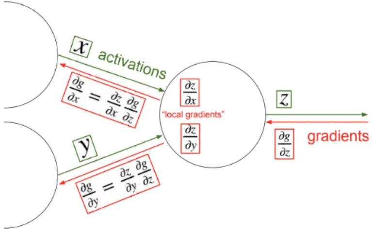
By evaluating the gradients of the loss function and using stochastic gradient descent (SGD) to minimize the loss, it is possible to find a mapping function 𝑓 ∈ 𝐹 which can map 𝑋 → 𝑌 consistent with the training data. This section describes the process of backpropagation which efficiently computes gradients of scalar valued functions with respect to their inputs. For any feed forward network including deep neural networks, the prediction y ˆ𝑦 for any input 𝑥 is made by passing the information forward through the network. During training, the forward pass continues onward until it produces a scalar cost value. The backpropagation, allows the information from the cost to flow backwards in order to compute the gradients. Consider the example shown in Figure 3.1.

During forward pass𝑥 and𝑦 take on specific (numerical) values and the vector (or scalar) 𝑧 is computed using some fixed function (e.g. 𝑧 = 𝑥 𝑦). Notice that it is possible immediately compute the Jacobian matrices𝑑 𝑧/𝑑𝑥 and𝑑 𝑧/𝑑𝑦of this transformation using calculus, because of the knowledge of what function 𝑧 is computing in the forward pass. These tell us what first order influence𝑥and𝑦have on the value of𝑧. The value𝑧goes off into a computational graph and eventually at the end of the graph the total loss𝑔(a scalar) is computed. The backward pass proceeds in the reverse order, recursively applying the chain rule to find the influence of all inputs of the graph on the final output. In particular, this computational unit finds out what𝑑𝑔/𝑑 𝑧is, telling us how 𝑧influences the final graph output. The chain rule states that to backpropagate this we should take the global gradient on𝑧, 𝑑𝑔/𝑑 𝑧and multiply it onto the local gradients for each input. For example, the global gradient for𝑥 will become𝑑𝑔/𝑑𝑥 = 𝑑 𝑧/𝑑𝑥 𝑑𝑔/𝑑 𝑧. If𝑥 , 𝑧 are vectors then this is a single matrix-vector multiplication. The gradient is then recursively chained, in turn, through the functions that produced the values of𝑥and𝑦until the inputs are reached. In neural network applications, the inputs we are interested in are the parameters, and their gradient tells us which way they should be nudged to decrease the loss.

Computational Graph Representation: Instead of thinking of the computational process of a Neural Network as a linear list of operations it is more intuitive to think about the function from inputs to outputs as a directed acyclic graph (DAG) of operations, where vectors flow along edges and nodes represent differentiable transformations that consume some number of vectors and combine them to one vector that then flows to other nodes. Most implementations of backpropagation organize the code base around a Graph object that maintains the connectivity of operations (also called gates, or layers) and a large collection of possible operations. Both Graph and Node objects implement two functions: forward() and backward(). The Graph’s forward() iterates over all nodes in the topological order and calls their forward(), and its backward() iterates in the reverse order and calls their backward(). Each Node computes its output with some function during its forward() call,

and in backward() it is given the gradient of the loss function with respect to its output and returns the ’chained’ gradients on all of its inputs. Here the ’chained implies taking the gradient on its output and multiplying it by its own local gradient (the Jacobian of this transformation). This gradient then flows to its children nodes that perform the same operation recursively. As a last technical note, if the output of a node is used in multiple places in the graph then correct behavior by the multivariable chain rule is to add the gradients during backpropagation along all branches. This would be handled in the Graph object.

3.3. REGULARIZATION

Unfortunately, optimizing Equation 3.2 instead of Equation 3.1 poses challenges. For instance, consider a function 𝑓 that maps each 𝑥𝑖 in the training data to its 𝑦𝑖 but returns zero everywhere else. This would be a solution to Equation 3.2 (for any sensible loss function 𝐿 that achieves a minimum value when 𝑦 = 𝑦ˆ), but we would expect very high loss for all other points in𝐷that are not in the training set. In other words, we would not expect this function to generalize to all (𝑥 , 𝑦)∼ 𝐷. An additional concern is that there may be many different functions that all achieve the same loss under Equation 2.2 (so there is no unique solution), but their generalization outside of the training data could vary. If there is only training data then the challange is to choose among an entire set of 𝑓 ∈ 𝐹 that all achieve the same loss in Equation 3.2? Both of these concerns can be alleviated by using regularization. There are a couple of regularization types in machine learning, but the followin are popular in deep learning.

3.3.1. L2 Regularization. This regularization works by adding the term 𝑅to the objective: 𝑓∗ =argmin 𝑓∈𝐹 1 𝑛 𝑛 Õ 𝑖=1 𝐿(𝑓(𝑥_𝑖), 𝑦_𝑖) +𝑅(𝑓) (3.4)

where𝑅is a scalar-valued function that encodes preference for some functions over others, regardless of their fit to the training data. This addition can be partly justified as following the principle of Occam’s razor, which could be stated as: ’Suppose there exist two explanations for an occurrence. In this case the simpler one is usually better’. Put in another way, the regularization is a measure of complexity of a function. Together with the regularization term, the objective in Equation 2.3 encourages simple solutions that also fit the training data well, and its intended effect is to some extent compensate for the discrepancy between the objective in Equation 3.2 and Equation 3.1.

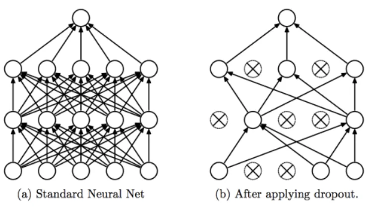
3.3.2. Dropout. The key idea is to randomly drop units (along with their connec-tions) from the neural network during training as shown in Figure 3.2. This prevents units from co-adapting too much. During training, dropout samples from an exponential number of different ’thinned’ networks. At test time, it is easy to approximate the effect of averaging the predictions of all these thinned networks by simply using a single unthinned network that has smaller weights. This significantly reduces overfitting and gives major improvements over other regularization methods.

Figure 3.2. Dropout Neural Net Model. Left: A standard neural net with 2 hidden layers. Right: An example of a thinned net produced by applying dropout to the network on the left. Crossed units have been dropped.

3.4. CONVOLUTIONAL NEURAL NETWORK

Convolutional neural networks (CNNs) are a class of deep neural networks designed for handling data with some spatial topology (e.g. images, videos, sound spectrograms in speech processing, character sequences in text, or 3D voxel data). In each of these cases an input example 𝑥 is a multi-dimensional array (i.e. a tensor ). CNNs use relatively little pre-processing compared to other supervised learning methods. This implies that the network learns the filters that in traditional algorithms were hand-engineered which gives a major advantage over other traditional algorithms.

Figure 3.3. CNN model. Illustration of convolving a 5x5 filter (which we will eventually learn) over a 32x32x3 input array with stride 1 and with no input padding. The filters are always small spatially (5 vs. 32), but always span the full depth of the input array (3). There are 28 x 28 unique positions for a 5 x 5 filter in a 32 x 32 input, so the convolution produces a 28 x 28 activation map, where each element is the result of a dot product between the filter and the input. A convolutional layer has not just one but a set of different filters (e.g. 64 of them), each applied in the same way and independently, resulting in their own activation maps. The activation maps are finally stacked together along depth to produce the output of the layer (e.g. 28 x 28 x 64 array in this case).

3.4.1. Conv Layer. The core computational building block of a Convolutional Neural Network is the Convolutional Layer (or the CONV layer) which takes an input tensor and produces an output tensor by convolving the input with a set of filters. For instance, consider the example shown in Figure 3.3. The input is a color image with dimensions

32x32x3 while the choice of filter is 5x5x3 (= 75 parameters which are trainable). The convolution happens by sliding the filter across the spatial points of the input tensor (one step at a time i.e. stride = 1) and computing the dot product between local values of𝑋 and 𝑤. This produces an activation map which will have the dimension 28x28x1. It is common to use multiple such filters in each layer (say 32) and the output will have a dimension of 28x28x32. Also, for very deep CNNs (which is common for CNNs) it is necessary to maintain the dimensions so as to be able to stack multiple layers. For this purpose, the input at each layer is padded with a border of zeros. If a pad of 2 is added to the input tensor𝑥in Figure 3.3 and the convolution is performed with same stride value (stride = 1), the resulting activation will have the same height and width as that of input tensor x i.e. 32x32x32. As the complete architecture is optimized using loss, each filter will develop the capacity to look for certain local features in the input tensor𝑥. Steps performed during conv operation:

1. Input a tensor𝑥 with dimensions𝑊₁x𝐻₁x𝐶₁

2. Define configuration of conv: stride 𝑠, pad 𝑝, number of filters𝐾 and spatial extent of filter𝐹.

3. Produce a activation map with dimensions𝑊₂x𝐻₂x𝐶₂where𝑊 =(𝑊₁−𝐹+2𝑃)/𝑆+1,

𝐻₂= (𝐻₁−𝐹 +2𝑃)/𝑆+1 and𝐶₂=𝐾.

3.4.2. Pool Layer. In addition to convolutional layers, to further control overfitting it is common to use pooling layers that decrease the size of the representation with a fixed downsampling transformation (i.e. without any parameters). In particular, the pooling layers operate on each channel (activation map) independently and downsample them spatially. A commonly used setting is to use 2x2 filters with stride of 2, where each filter computes the max operation (i.e. over 4 numbers). The result is that an input tensor is downscaled exactly by a factor of 2 in both width and height and the representation size is reduced by a factor of 4, at the cost of losing some local spatial information.

3.4.3. ConvNet Architectures. Finally, a convolutional network is built by stacking convolutional layers and possibly introducing pooling layers to control the computational complexity of the architecture. A typical convolutional neural network architecture that processes images might take the form [INPUT, [CONV, CONV, POOL] x 3, F C, F C]. Here, INPUT represents a tensor of a batch of images (e.g. [100 x 32 x 32 x 3] for a batch of 100 32 x 32 color images) CONV is a convolutional layer with 3x3 filters applied with padding of 1 and stride of 1, POOL stands for a typical 2x2 filter max pooling layer with stride of 2, and FC are fully-connected layers, where the last one computes the logits of different classes just before a softmax classifier. In this architecture the spatial size of the input is reduced by a factor of 2 in both width and height after each POOL layer, so after the third POOL layer the spatial size of the representation along width and height would be 4x4.

3.5. RECURRENT NEURAL NETWORK

In many practical applications the input or output spaces contain sequences. For example, sentences are often modeled as a sequence of words, where each word is encoded as a one-hot vector (i.e. a vector of all zeros except for a single 1 at the index of the word in a fixed vocabulary). A recurrent neural network (RNN) is a connectivity pattern that processes a sequence of vectors {𝑥₁, ..., 𝑥_𝑇} using a recurrence formula of the form

ℎ𝑡 = 𝑓𝜃(ℎ𝑡−1, 𝑥𝑡), where 𝑓 is a function that we describe in more detail below and the same parameters𝜃are used at every time step, allowing us to process sequences with an arbitrary number of vectors. The hidden vector ℎ_𝑡 can be interpreted as a running summary of all vectors 𝑥 until that time step and the recurrence formula updates the summary based on the next vector. It is common to either use ℎ₀ = 0, or to treat ℎ₀ as parameters and learn

the starting hidden state. The precise mathematical form of the recurrence(ℎ_𝑡−1, 𝑥_𝑡) →ℎ_𝑡

Figure 3.4. RNN architecture designs. An ordinary neural network (left) might take an input vector (red), transform it through some hidden layer (green), and produce an output vector (blue). In these diagrams boxes indicate vectors and arrows indicate functional dependencies. Recurrent neural networks allow us to process sequences of vectors, for example: 1) at the output, 2) at the input, or 3) both either serially or in parallel. This is facilitated by a recurrent hidden layer (green) that manipulates a set of internal variables ht based on previous hidden stateℎ_𝑡−1and the current input using a fixed recurrence formula ℎ_𝑡 = 𝑓_𝜃(ℎ_𝑡−1, 𝑥_𝑡), where𝜃 are parameters we can learn.

That is, the previous hidden vector and the current input are concatenated and transformed linearly by the parameters𝑊. Note that this is equivalent to instead writing ℎ𝑡 =𝑡 𝑎𝑛 ℎ(𝑊𝑥 ℎ𝑥𝑡 +𝑊ℎ ℎℎ𝑡−1), where the two matrices𝑊𝑥 ℎ, 𝑊ℎ ℎ concatenated horizontally are equivalent to the matrix𝑊 above. These equations omit the additional bias vector for brevity. The tanh nonlinearity can also replaced with ReLU. If the input vectors𝑥_𝑡 have dimension𝐷 and the hidden states dimension𝐻 then𝑊 is a matrix of size [𝐻x (𝐷+𝐻)]. Interpreting the equation, the new hidden states at each time step are a linear function of elements of 𝑥_𝑡, ℎ_𝑡−1 and squashed by non-linearity. The vanilla RNN has a simple form,

but unfortunately, the additive interactions are a weak form of coupling [32,33] between the inputs and the hidden states and the functional form of vanilla RNN leads to undesirable dynamics during backpropagation [6] (In particular, the gradients tend to either vanish or explode over long time periods). The exploding gradient concern can be alleviated with a heuristic of clipping the gradients at some maximum value [7], but the RNNs still suffer from the vanishing gradient problem.

3.6. LONG SHORT-TERM MEMORY

The LSTM [8] recurrence is designed to address the limitations of the vanilla RNN. Its recurrence formula has a form that allows the inputs 𝑥_𝑡 and ℎ_𝑡−1 interact in a

more computationally complex manner that includes multiplicative interactions, and the LSTM recurrence uses additive interactions over time steps that more effectively propagate gradients backwards in time [8]. In addition to a hidden state vector ℎ_𝑡, LSTMs also maintain a memory vector𝑐_𝑡. At each time step the LSTM can choose to read from, write to, or reset the cell using explicit gating mechanisms. The precise form of the update is as shown in Figure 3.5.

Figure 3.5. LSTM Equations.

Here, the sigmoid function sigm and tanh are applied element-wise, and if the input dimensionality is𝐷and the hidden state has𝐻units then the matrix𝑊has dimensions [4𝐻 x(𝐷+𝐻)]. The three vectors𝑖, 𝑓 , 𝑜 ∈𝑅𝐻are thought of as binary gates that control whether each memory cell is updated, whether it is reset to zero, and whether its local state is revealed in the hidden vector, respectively. The activations of these gates are based on the sigmoid function and hence allowed to range smoothly between zero and one to keep the model differentiable. The vector𝑔 ∈ 𝑅𝐻 ranges between -1 and 1 and is used to additively modify the memory contents. This additive interaction is a critical feature of the LSTMs design, because during backpropagation a sum operation merely equally distributes gradients. This

allows gradients on the memory cells𝑐 to flow backwards through time uninterrupted for long time periods, or at least until the flow is disrupted with the multiplicative interaction of an active forget gate.

Example: Character-level Language Modeling. Character-level language models are a commonly studied interpretable testbed for sequence learning. In this setting, the input to the RNN is a sequence of characters from some text (e.g. ’cat sat on a’) and the network is trained to predict the next character in the sequence (’m’ in this example, the first letter of ’mat’). Concretely, assuming a fixed vocabulary of𝐾 characters we encode all characters with 𝐾-dimensional one-hot vectors {𝑥𝑡}, 𝑡 = 1, ..., 𝑇 , and feed these to the network to obtain a sequence of𝐻-dimensional hidden vectors{ℎ_𝑡}. To obtain predictions for the next character in the sequence we further project the hidden states to a sequence of vectors {𝑦_𝑡}, where 𝑦_𝑡 =𝑊_𝑦ℎ_𝑡 and𝑊_𝑦 is a [𝐾 x 𝐻] parameter matrix. These vectors are the logits of the next character (so the probabilities are obtained by passingthese through a softmax function) and the objective is to minimize the average cross-entropy loss over all targets.

3.7. TRAINING SUMMARY

Data preparation. First, obtain a dataset that is made up of a set of pairs (𝑥 , 𝑦) where 𝑥 is some input example and 𝑦 is a label. The data is then split into three folds, commonly a training, validation and test fold (common proportions could be 80%, 10%, 10% respectively). The training fold is used for optimizing the parameters with backpropa-gation, the validation fold for hyperparameter optimization, and the test fold for evaluation (discussed below in more detail). Data preprocessing. Preprocessing the data can help im-prove convergence of neural networks [5]. For images, common preprocessing techniques involve standardizing the data (subtracting the mean and dividing by the standard deviation individually for every input dimension of𝑥), or at the very least subtracting the mean. It is

critical to estimate these statistics only on the training data, and using these fixed statistics to process the validation and test data, as this appropriately simulates the deployment of the final system into a real-world application.

Optimization. A default recommendation is to use Adam [4] for optimization, with learning rates of approximately 1e3, the coefficient of first moment of 0.9 and second moment 0.99. It is often beneficial to anneal the learning rate during the course of training by approximately a factor of 100 by the very end of training, but it is common to decay the first time only after half of the training is finished. During optimization it is almost always a good idea to use Polyak averaging [7], where we keep track of an averaged parameter vector𝜃_{𝑎 𝑣 𝑔} (e.g. 𝜃_{𝑎 𝑣 𝑔} = 0.999𝜃_{𝑎 𝑣 𝑔} + 0.001𝜃) after every parameter update and use𝜃_{𝑎 𝑣 𝑔} to compute the validation performance and when saving the model checkpoint to file.

4. SYSTEM ARCHITECTING APPROACH FOR DEEP LEARNING

This section introduces the framework required to simplify the steps necessary to perform the neural architecture search. It also presents a case study showing the use of framework to effectively explore large design space by automating certain model construc-tion, alternative generaconstruc-tion, and assessment. The framework exploits the system architecting principles for exploring different types of deep learning architectures related to computer vision and natural language processing. It provides the architect necessary capabilities to modify the search space, participating layers and objectives based on the requirements.

The application of framework to find an optical architecture for CIFAR-10 dataset show the evolution of neural architectures with minimized human participation. Despite significant computational requirements, it is now possible to design architectures as good as a state-of-the-art models simply by defining the search space, layers and objectives. Experimental results show that evolving architectures on a well defined search space can produce multiple architectures that are on par with state-of-the-art models while removing the manual hours spent on designing the architecture. These results also show that there is a promise to further the improve the overall architecture search by improving the evolutionary process.

4.1. OUTLINE

With the success of recent neural architecture search (NAS) approaches in deep learning, it is evident that the evolved designs are capable of outperforming the human made designs. So far, all the NAS approaches use almost identical search spaces and optimized on objective/s to produce an optimal architecture. In general, the neural architecture search (NAS) consists of three phases as shown in Figure 4.1. (1) The search space (𝑆) encapsulates the logical representation of different architectures that are possible using the

defined operations. The range of values used for representing different architectures depends on the architect. The current NAS approaches either use binary format or integer format to define the architectures. (2) The search strategy defines the optimization technique and responsible for building the graphs for different architecture based on the search space (𝑆). The most popular search strategies include genetic algorithms, reinforcement learning and differential approach. (3) The performance evaluation performs training & validation. It also calculates the overall objective value which is used by the search strategy to generate better architectures. This step is the most time consuming part of the entire search process as each architecture is trained and validated for a set of epochs. Once the architectures are evaluated, the validation accuracy is combined with other objectives to get an overall objective score. This process is repeated until a stopping criteria is reached.

Figure 4.1. Illustration of neural architecture search method. The search strategy generates an architecture from search space𝑆. The performance is calculated using the performance evaluation method and the value is returned to the search strategy.

While this approach is successful on standard datasets such as CIFAR-10/100 and IMAGENET, the real-world application of these approaches usually face far more constraints in the form of computational complexity, resources and time. Therefore, it is essential to have the capability to change the parameters of NAS depending on the requirements of the architect. This implies that for successful application of NAS on new datasets, there should be (1) Fleible architecture search space: Based on the dataset and available computation, the architect should have the freedom to specify the search space rather than to use a space that is constrained to a block. The framework presented in this section allows the architect

to explicitly design the search space based on problem requirements. (2) Multi-objective capability: Models that are designed for deployment on real-world devices are generally less expensive in terms of computation. This is achieved by having a trade-off between the accuracy and compute. To facilitate this process, the framework incorporates multi-objective optimization such that the designed models follow the trade-off constraints. (3) Flexible layer combinations: Based on type of deep learning model and dataset features, the choice of layers may vary in terms of filter size, number of filters and type of layers. The framework provides this capability to the architect by inputting the layer configurations before the start of the search process.

4.2. RELATED WORK

System architecting approaches, applied in design, analysis and optimization have flourished in various domain specific disciplines [4, 14, 21]. Our approach aims to use these capabilities in the field of deep learning to reduce the human effort required to design the architectures by considering each layer as a system and finding optimal connectivity between input and output.

The idea of using evolution to learn neural networks dates back to 2001[11]. At-tempts were made to design or optimize neural networks using evolutionary algorithms, reinforcement learning and other machine learning approaches[23, 29]. In recent years, these approaches resurfaced as the deep learning architectures became deeper thereby in-creasing the search space significantly. Initial approaches include the design architectures that can overcome the man-made models[2, 26, 27]. The prominent feature of these attempts is to design complete architectures and optimize them based on the validation accuracies. Since it included the design of complete architecture, they are computationally expensive and also they did not have much success when compared to the state-of-the-art models except for [2, 24].

In order to reduce the computational complexity and be able to search for optimized architectures in the design space, it is more advantageous to build a novel search space that has the capability to do both. In [35], the authors showed that by using a small and efficient search spaces, we can build highly efficient architectures. Our approach takes inspiration from [35] and [24] to develop a search space that is capable of designing very deep architectures. By using a system architecting approach, we can have the desired search space for multiple objectives [1, 5] which is more generic.

4.3. FRAMEWORK

The systems architecting approach to build a framework for NAS is implemented in four phases as shown in Figure 4.2. The configuration of each phase will define the overall NAS problem that needs to be solved.

Figure 4.2. Outline of NAS framework. The encoding defines the search space for the architectures. The mutation generates new architectures based on search space and objective values. The multi-objective function calculates overall objective value based on different objectives provided by the architect. Lastly, the trade-off defines helps the architect to choose the most optimal solution.

4.3.1. Encoding. Since deep learning models can be viewed as stack of computa-tional blocks that define layer wise computation, each layer can be encoded using a unique representation. Similarly, the inputs to each layer can just be the output of previous layer

[3] or outputs of multiple layers as in [4]. Therefore, the entire encoding scheme of the architecture is a combination of both operation encoding (𝐴_{𝑜 𝑝 𝑠}) for layer wise operations and interface encoding(𝐴_{𝑖 𝑓}) for connectivity between the layers.

𝐴= 𝐴_{𝑜 𝑝 𝑠} +𝐴_{𝑖 𝑓} (4.1)

4.3.1.1. Operation encoding. The operation encoding is represented in a sequen-tial format as whose length is equal to the number of layers on which the search is applied. If𝑂represent the set of chosen operations, the encoding is given by

𝐴_{𝑜 𝑝 𝑠} =[𝑜(1) 𝑖 , 𝑜(2) 𝑖 , 𝑜(3) 𝑖 , ..., 𝑜(𝐿) 𝑖 ] (4.2)

where𝑖∈𝑂 and𝐿is the number of layers.

Figure 4.3. Encoding for wide architecture. It is the same formulation used in state-of-the-art NAS approaches.

4.3.1.2. Interface encoding. The interface encoding(𝐴_{𝑖 𝑓})defines the connectivity among the layers. So far, state-of-the-art deep learning models are based on two types: (1) wide models such as inception & googleNet and (2) deep models such as ResNet and DenseNet. Combining both of these designs explodes the search space and it becomes

difficult to find optimal architecture using reasonable computation. To prevent such scenario, the framework uses either a wide design or deep design based on the architect’s requirement. Since both these designs have significant differences in connectivity, the framework provides unique encoding approach for both of them as descibed below:

Wide Design: The wide design is used in almost all of the state of the art NAS approaches [12]. Each operation chooses only one input from the set of available options to generate a complete architecture as shown in Figure 4.3. In general, only two previous layersℎ𝑡andℎ𝑡−1are used to design the overall NAS layer. Therefore, the choice of inputs

can be represented by unique integers for each layer. If𝑇 represents the set of previous layers, the general formulation for wide design interface encoding is given by

𝐴_{𝑖 𝑓} = [𝑐(1) 𝑗 , 𝑐 (2) 𝑗 , 𝑐 (3) 𝑗 , ..., 𝑐 (𝐿) 𝑗 ] (4.3)

where 𝑗 ∈𝑇 and𝐿is the number of layers.

Deep Design: The deep design capability in this framework is inspired by the popular ResNet[16] and DenseNet[17] architectures. Unlike wide design, deep architectures have a lot of interconnections and it is difficult to represent the architectures using integer format. Therefore, a one-hot encoded approach is more suitable as shown in Figure 4.4. In this encoding, the presence of connection is represented by 1 while 0 represents no connection. The formulation for deep design is given by

𝐴_{𝑖 𝑓} = [(𝑝1),(𝑝1, 𝑝2), ...,(𝑝1, 𝑝2, ..., 𝑝𝐿)] (4.4)

where𝑝 ∈0/1

4.3.2. Sampling. The main idea of the sampling is to (1) generate feasible archi-tectures based on search strategy and encoding. (2) improve architecture design using past knowledge and prevent local minima.

Figure 4.4. Encoding for deep architecture.

4.3.3. Architecture Evaluation and Trade-off. Each new architecture generated using the sampling process is trained and evaluated on validation accuracy by default. The optimal architecture is therefore the one which has highest validation accuracy. If additional objectives are added, the architect is responsible for identifying the trade-off between the validation accuracy and other objectives. Section 6 discusses this concept in detail.

4.4. CASE STUDY

In this section, the proposed NAS framework is used to design a dense architecture for an image classification problem to demonstrate the effectiveness of framework for finding optimal architecture. For the sake of quantitatively comparing the performance with the state-of-the-art models, only validation accuracy is used as the overall objective.

4.4.1. Dataset. The CIFAR-10 dataset is a collection of images each consisting of one of the 10 different classes - airplanes, cars, birds, cats, deer, dogs, frogs, horses, ships, and trucks. It consists of 60,000 32x32 images that are uniformly distributed among all classes (6000 images for each class) and is commonly used to develop deep-learning object detection algorithms. Because of the low resolution images (32x32), the CIFAR-10 dataset allows the architects to test different types of algorithms and compare their performance with minimal computation. Figure 4.5 shows few examples of CIFAR-10 dataset.

Figure 4.5. Samples from CIFAR-10 dataset.

4.4.2. Modelling the Architecture Using Framework. The image classification models generally consist of different types of layers that provide different capabilities to the overall architecture. Table 4.1 shows the capabilities provided by different layers that are used in CNN. The goal is to use the capabilities of the layers mentioned in Table 4.1 and design a hybrid architecture that can give optimal performance i.e. maximum validation accuracy.

4.4.2.1. Encoding. As shown in Figure 4.2, the first step in using the framework is choose an encoding format for the architecture search. Since the current objective is to design a deep and dense model, it uses the encoding format defined in Equation 4.1 where 𝐴_{𝑖 𝑓} uses a deep design.

Table 4.1. Table showing layers and their capabilities

System/Layer Linear

transformation

Non-linear

transformation Regularization Parameter scaling

convolutional layer x - -

-pooling layer x - -

-activation layer - x -

-dropout - - x

-batch-normalization - - x x

In addition, as described in Section 2.2.2, using architecture search on a pre-determined template is more computationally feasible than on complete architecture. There-fore, the current architecture search is performed on the template as shown in Figure 4.6. The search process is applied only on a small part of the architecture called e-block. The e-blocks are separated by a transition layers which offer the necessary hierarchy necessary for the overall architecture.

Equation 4.2 shows that encoding requires a set of pre-defined operations which can be used in the architecture search. Based on the literature developed so far, each convolutional layer in a CNN design is often accompanied by a Relu activation - dropout with a probability of 0.8/1 and batch normalization. Therefore, the possibility of generation different operations for the search space lie in the convolutional layer.

If a convolutional layer is represented by conv_𝑤_ℎ_𝑛where𝑤is filter width, ℎis filter height and𝑛is number of filters. For this case study, the𝑤, ℎ∈ [1,3,5,7] while𝑛 ∈ [12,24,33,34]. This generates a total of 62 unique operations𝑂 such that𝑜_𝑖 ∈{1-62} in Equation 4.2.

Figure 4.6. Pre-Detemined architecture designs. The top model was used for evolution and the bottom model was used to train complete architecute.

4.4.2.2. Genetic algorithm for search strategy. The second step in the framework is to design a search strategy for performing the architecture search. Some of the popular search strategies include genetic algorithms, reinforcement learning and differential ap-proaches. This dissertation uses genetic algorithms as they are relatively simple to use and require less hyper-parameters as compared to other techniques.

Genetic algorithms are a type of evolutionary algorithms that are inspired by the theory of natural evolution. It reflects the process of natural selection by choosing only the fittest individuals for reproduction in order to give offspring for next generation. The individuals are represented by a genotype and the algorithm produces the offspring either by mutation or crossover. From the frameworks perspective, each sampled encoding represents a genotype which can be identified as a unique deep learning model and the evolution implies the generation of new offspring models from the best performing models.

Mutation: The mutation process of an architecture (𝐴), involves changing only a single random bit𝑞_𝑖. This is done to preserve the good properties of a survived architecture while providing an opportunity of trying out new possibilities. Since the gene representing the architecture has both binary and integer values, the change is performed based on location of the bit. If the location of the bit represents a binary format, the the bit is flipped. For the case of integer format, a new value is chosen from the available range of values. Figures 4.7,4.8, 4.9 and 4.10 show examples of different possible mutation based on encoding formats.

Figure 4.7. Interface mutation on a deep design.

4.4.3. Experiments and Results. In this section, we describe the experiments conducted to learn e-blocks using the method mentioned above. We used CIFAR-10 dataset to learn multiple top performing e-blocks. All our experiments were performed using an NVIDIA TITAN X GPU.

Figure 4.9. Interface mutation on a wide design.

The search process took over 2 weeks using a single GPU and covered 500 architec-tures. We ran our approach for 50 generation with a population size of 10. The crossover and mutation operations are performed in such a way that repeated architectures are not generated.

Pre-Processing on CIFAR-10: The CIFAR datasets consist of colored natural images with 32×32 pixels. CIFAR-10 (C10) consists of images drawn from 10 classes. The training and test sets contain 50,000 and 10,000 images respectively, and we hold out 5,000 training images as a validation set. We adopt a standard data augmentation scheme (mirroring/shifting) that is widely used for this datasets [12,17,18,32]. For pre-processing, we normalize the data using the channel means and standard deviations. For the final run we use all 50,000 training images and report the final test error at the end of training.