Land cover mapping in support of LAI and FPAR retrievals from
EOS-MODIS and MISR: classification methods and sensitivities to
errors
A. LOTSCH, Y. TIAN, M. A. FRIEDL* and R. B. MYNENI Department of Geography, Boston University, 675 Commonwealth Avenue, Boston, MA 02215, USA
(Received 3 January 2001; in final form 3 January 2002)
Abstract. Land cover maps are used widely to parameterize the biophysical properties of plant canopies in models that describe terrestrial biogeochemical processes. In this paper, we describe the use of supervised classification algorithms to generate land cover maps that characterize the vegetation types required for Leaf Area Index (LAI) and Fraction of Photosynthetically Active Radiation (FPAR) retrievals from MODIS and MISR. As part of this analysis, we examine the sensitivity of remote sensing-based retrievals of LAI and FPAR to land cover information used to parameterize vegetation canopy radiative transfer models. Specifically, a decision tree classification algorithm is used to generate a land cover map of North America from Advanced Very High Resolution Radiometer (AVHRR) data with 1 km spatial resolution using a six-biome classification scheme. To do this, a time series of normalized difference vegetation index data from the AVHRR is used in association with extensive site-based training data compiled using Landsat Thematic Mapper (TM) and ancillary map sources. Accuracy assessment of the map produced via decision tree classification yields a cross-validated map accuracy of 73%. Results comparing LAI and FPAR retrievals using maps from different sources show that disagreement in land cover labels generally do not translate into strong disagreement in LAI and FPAR maps. Further, the main source of disagreement in LAI and FPAR maps can be attributed to specific biome classes that are characterized by a continuum of fractional cover and canopy structure.
1. Introduction
Vegetation and land cover play a key role in terrestrial biogeochemical processes, and changes in land cover induced by human activity have profound implications for climate, the functioning of ecosystems, and biogeochemical fluxes at regional and global scales (Dickinson and Henderson-Sellers 1988, Lean and Warilow 1989). As a consequence, a wide range of problems require reliable and accurate information on global land cover, and in particular, the distribution and properties of vegetation. With the launch of the National Aeronautics and Space Administration’s (NASA) Terra platform, a new generation of satellite sensor data is now available. For example, the Moderate Resolution Imaging Spectroradiometer (MODIS) on-board
* Corresponding author; e-mail: [email protected]
International Journal of Remote Sensing
ISSN 0143-1161 print/ISSN 1366-5901 online © 2003 Taylor & Francis Ltd http://www.tandf.co.uk/journals
Terra is providing substantially improved data for land cover mapping relative to the heritage data provided by the Advanced Very High Resolution Radiometer (AVHRR) (Justiceet al. 1998). Further, the Multi-Angle Imaging Spectroradiometer (MISR) provides image data of the Earth’s surface with nine view angles for each pixel that will be particularly useful for retrieving information regarding the structural properties of vegetation canopies such as the Leaf Area Index (LAI) and the Fraction of Photosynthetically Active Radiation (FPAR) (Knyazikhinet al. 1998a).
There are three primary objectives of this paper. The first objective is to present results from remote sensing-based vegetation mapping in support of the Earth Observing System (EOS) MODIS and MISR LAI and FPAR algorithm (Knyazikhin et al. 1998a,b). This algorithm uses radiative transfer models to retrieve information about the biophysical characteristics of plants from reflected solar radiation. The parameterization of such radiative transfer models, however, is dependent on the structural properties of the plant canopy. Within this framework, the MODIS/MISR LAI/FPAR algorithm recognizes six structurally distinct biomes. In support of this effort a decision tree classification algorithm is used to create a land cover map of North America using a six-biome classification scheme (right column in table 1). The primary data source that was used to produce this map is a 12 month time series of AVHRR Normalized Difference Vegetation Index (NDVI) data from February of 1995 to January of 1996. The second objective is to compare the resulting biome map to maps produced by translating (cross-walking) existing 1 km maps of global land cover produced by the University of Maryland (UMD) (Hansenet al. 2000) and the Earth Resources Observation Systems (EROS) Data Center (EDC) (Loveland et al. 2000) to the six-biome scheme. The third objective is to examine the sensitivity of LAI and FPAR retrievals to uncertainties in land cover labels.
2. Background
2.1. Global vegetation and land cover mapping approaches
Because of the diversity of vegetation at global scales, accurate mapping and representation of terrestrial vegetation has been a challenge for many years. For Table 1. Comparison of the IGBP and six-biome classification schemes (Loveland et al. 1995, Myneniet al. 1997). Note that an additional non-vegetated class is included in the biome scheme. This class is used in the classification process, but is ignored in the LAI/FPAR retrieval algorithm.
1 Evergreen Needleleaf Forests (ENF) 1 Grasses and Cereal Crops (GCC) 2 Evergreen Broadleaf Forests (EBF) 2 Shrubs (SHR)
3 Deciduous Needleleaf Forests (DNF) 3 Broadleaf Crops (BCR) 4 Deciduous Broadleaf Forests (DBF) 4 Savannas (SAV) 5 Mixed Forests (MXF) 5 Broadleaf Forests (BLF) 6 Closed Shrubland (CSH) 6 Needleleaf Forests (NLF) 7 Open Shrubland (OSH) 7 Non-Vegetated (NV) 8 Woody Savannas (WSA)
9 Savannas (SAV) 10 Grasslands (GRL)
11 Permanent Wetlands (PWL) 12 Croplands (CRL)
13 Urban and Built-up (URB) 14 Cropland Mosaics (CRM) 15 Snow and Ice (SNI)
16 Barren or Sparsely Vegetated (BSV) 17 Water Bodies (WAT)
example, Townshendet al. (1991) compared existing maps of global vegetation and showed that estimates of vegetation distribution from common sources varied consid-erably. While such databases have obvious limitations, until recently they represented the state of the science for parameterizing land properties in global scale process models.
There is wide consensus that remotely sensed data can provide an accurate and repeatable means of land cover mapping and monitoring, especially with respect to areas with changing land use and land management activities (Townshend et al. 1991, Runninget al. 1994). In particular, remote sensing-based approaches are able to exploit distinct spectral properties from different land cover types and temporal information related to phenological dynamics in vegetation (Justice et al. 1985, Loveland et al. 1991). Prior to the launch of Terra, most research on global land cover mapping has used data collected by the AVHRR instrument onboard the National Oceanic and Atmospheric Administration (NOAA) series of satellites (Justiceet al. 1985, Runninget al. 1994, Lovelandet al. 1995).
Although recent work has provided promising results, it must be noted that the utility of AVHRR data for land cover applications is limited by high levels of atmospheric noise, lack of onboard calibration, and limited spectral information (Moody and Strahler 1994, Zhu and Yang 1996, Cihlar et al. 1997). The MODIS instrument is expected to overcome many of these limitations (Strahler et al.1999, Friedl et al. 2000b). Specifically, MODIS provides superior spectral and spatial resolution, atmospheric correction, and calibration relative to AVHRR data (Runninget al. 1994, Barneset al. 1998, Justiceet al. 1998).
2.2. Remote sensing of L AI and FPAR
The relationship between NDVI and LAI and FPAR has been well established through both theoretical and empirical studies. However, the utility of this relation-ship depends on the sensitivity of these variables to canopy characteristics (Myneni et al. 1997). While FPAR exhibits a positive linear relationship with increasing NDVI, LAI is non-linearly related to NDVI, saturating at LAIs of 3–6, depending on the vegetation type. In order to estimate LAI and FPAR from remotely sensed data, canopy structural types must be defined that exhibit unique NDVI–LAI or FPAR relations from one another. Therefore many classification schemes which are based on ecological, botanical, or functional metrics are not necessarily suitable for LAI and FPAR retrieval.
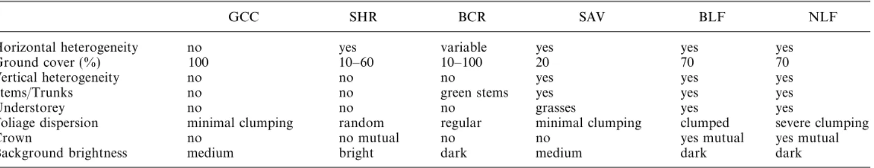
Most LAI and FPAR retrieval algorithms are based on inversion of radiative transfer models, which simulate radiation absorption and scattering in vegetation canopies. A review of such models can be found in Myneni et al. (1995). The algorithm being used to retrieve LAI and FPAR from MODIS and MISR data is based on six distinct plant structural types ( biomes) defined by Myneniet al. (1997). The definitions and properties of the six biomes as they relate to radiative transfer are presented in table 2. The MODIS/MISR LAI and FPAR retrieval algorithm relies on a database describing the global distribution of these biomes to invoke different radiative transfer models. Note that a non-vegetated class (class 7) is included in the classification process in addition to the six biome types. This class, however, does not permit retrievals of LAI and FPAR and is therefore not included in the discussion below regarding the sensitivity of LAI and FPAR retrievals to land cover classification errors.
A.
L
otsch
et
al.
Table 2. Canopy structural attributes of global land covers from the viewpoint of radiative transfer modelling (Myneniet al. 1997).
GCC SHR BCR SAV BLF NLF
Horizontal heterogeneity no yes variable yes yes yes
Ground cover (%) 100 10–60 10–100 20 70 70
Vertical heterogeneity no no no yes yes yes
Stems/Trunks no no green stems yes yes yes
Understorey no no no grasses yes yes
Foliage dispersion minimal clumping random regular minimal clumping clumped severe clumping
Crown no no mutual no no yes mutual yes mutual
2.3. T ree-based classification algorithms
A variety of different techniques are used currently to classify remotely sensed data for land cover and vegetation mapping applications. Traditionally, land cover mapping approaches have used either parametric supervised classification algorithms or unsupervised classification algorithms. These latter algorithms employ clustering techniques to identify spectrally distinct groups of data (Schowengerdt 1997), and have been used widely with high spatial resolution imagery such as Landsat or SPOT. Global land cover classification efforts, however, have generally employed coarse spatial resolution data from the AVHRR (Lovelandet al. 2000). These efforts have used unsupervised clustering in conjunction with ancillary data and manual labelling (Loveland et al. 1991), maximum likelihood classification (DeFries and Townsend 1994), or hierarchical classification logic based on structural and biophysical parameters (Running et al. 1995). More recent approaches include applications of neural networks, including fuzzy neural networks (Carpenteret al. 1992, Gopal and Woodcock 1996).
Recently, decision tree algorithms have been used to classify global datasets with promising results (DeFrieset al. 1998b, Friedlet al. 1999, Hansen et al. 2000). Decision trees are computationally efficient and flexible, and also have an intuitive simplicity (Safavian and Landgrebe 1991). They therefore have substantial advant-ages in remote sensing applications (Friedl and Brodley 1997). Tree-based methods are categorized as supervised techniques and a training dataset is required from which the decision tree is estimated.
3. Methodology
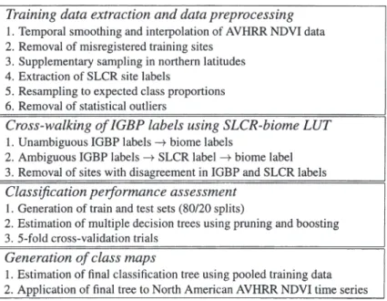
The analysis presented below involves six main components. Section 3.1 describes the data that was used to generate land cover maps using the six-biome classification scheme. Section 3.2 discusses data pre-processing and outlier removal procedures. Section 3.3 explains the steps that were taken to cross-walk existing classification products into biome classes throughout the analysis, and §3.4 describes the classifica-tion and accuracy assessment process. Finally, §3.5 shows how the class map was compared to existing global land cover maps and §3.6 describes how the LAI and FPAR retrievals were performed and assessed, focusing on the sensitivity of LAI and FPAR to uncertainties in land cover information. The steps taken to generate the biome map (§3.1–3.4) are summarized in figure 1.
3.1. Data
The classification analyses presented below were based on a 12 month AVHRR NDVI time series. The dataset was composed of monthly composited NDVI data covering the time period between February 1995 and January 1996. The training data used for this analysis were extracted from a database of global land cover training sites that was compiled by the MODIS Land Cover and Land-Cover Change group at Boston University (BU) (Strahler et al. 1999, Friedl et al. 2000b). This database contained approximately 1000 sites in North America and has under-gone several iterations of quality control. Each site in the database possessed an areal extent ranging between 2 and 100 km2, a label assignment defined by the International Geosphere–Biosphere Programme (IGBP) classification scheme ( left column in table 1) (Loveland and Belward 1997), and where possible, a set of biophysical parameters that describe the ecological and biophysical conditions of the site (Muchoneyet al. 1999). The label and attribute assignments were performed
Figure 1. Data processing flow for the generation of the biome class map.
using recent Landsat Thematic Mapper (TM) imagery along with ancillary data sources such as existing paper or digital maps, literature sources, aerial imagery, and ground information provided by collaborating science teams. In addition, site labels extracted from the Seasonal Land Cover Characterization (SLCR) database (Lovelandet al. 2000), were used as an additional predictive variable in the classifica-tion process. Each training site was registered to coordinates in the Universal Transverse Mercator (UTM) Projection, converted to a raster image format with a 30 m resolution, aggregated to a 1 km resolution, and reprojected to the Integerized Sinosoidal Grid (ISG) Projection used for EOS products. Uncertainties in the training site database, that were still present despite multiple iterations of quality control, were reduced using a method described in the next section.
The global land cover maps published by UMD and EDC are used within the analysis for stratified sampling, supplementary training site selection, and for a benchmark comparison of the final class map. The EDC classification follows the IGBP scheme and includes 17 classes of land cover and vegetation. The classification scheme used by UMD basically follows the IGBP classification logic. However, three IGBP classes are not included in the UMD scheme: snow and ice, permanent wetland, and cropland mosaic. Therefore these three classes were excluded from further analysis. Both maps were created using AVHRR data from 1992 and 1993 and have a spatial resolution of 1 km. For detailed descriptions of the classification algorithms used to generate the UMD and EDC datasets, see Hansenet al. (2000), Lovelandet al. (1995), (2000).
3.2. Data pre-processing
Because of data quality issues related to radiometric quality, errors in geometric rectification, cloud screening, and labelling errors by analysts, the site database was carefully screened prior to using it for analyses. This was accomplished in four steps. First, missing values in the AVHRR NDVI data (data dropouts), particularly in
northern latitudes, were filled using temporal smoothing and interpolation routines. Data dropouts were typically limited to a few months, which allowed smooth interpolation of NDVI profiles. Extremely distorted NDVI profiles arising from interpolation were subsequently eliminated in the outlier detection process described below. The number of pixels with interpolated NDVI trajectories in the training data was therefore minimized.
Second, due to misregistration of some of the Landsat TM scenes, not all sites could be used in the analysis. Out of the approximately 1000 sites, only 665 were used. This issue was particularly pronounced at high latitudes. As a result, land areas in the northern part of the continent were undersampled. To compensate, 32 new training sites were added based on areas of agreement between the UMD and EDC maps. This step was justified based on the assumption that confidence in class labels is high where two independently generated maps agree. This approach used the SLCR database as a basis for stratified sampling to ensure that land covers of different heterogeneity and phenology were captured. The sites were chosen randomly across the undersampled region with sufficient distance between each other to remove the effect of spatial autocorrelation between sites.
Third, to compensate for oversampled classes in the site database, the training data were resampled to reflect the expected proportions of land cover based on the proportions of each class in the UMD and EDC maps for North America. This step accounts for the fact that decision tree algorithms tend to overpredict classes that are oversampled. To reduce this bias, a random sample (i.e. a sub-sample) propor-tional to the estimated frequency of the class on the ground was generated and used for further analysis for those classes that were oversampled in the training data. Note that this step was primarily intended to scale down the effect of agricultural land cover classes (IGBP 12 and 14), which were substantially over-represented in the training database.
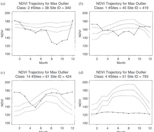
Finally, a key step in developing the training site database was to remove statistical outliers to avoid unwanted confusion in the classification algorithm and results. To do this, a two-step generalized gap test for multivariate outlier detection was performed (Rohlf 1975). This method constructs a minimum spanning tree based on distance in multidimensional feature space and removes NDVI trajectories where NDVI values fall outside of one standard deviation (SD) for 6 or more months. This procedure required two steps. In the first step, outliers in each training site were removed with the intent of increasing the homogeneity in each site. In the second step, sites were identified as outliers within each class to decrease within-class heterogeneity, while retaining the natural class variability at the same time. Examples of representative outliers are shown in figure 2. Note that outliers are characterized by NDVI trajectories that deviate substantially from the class mean. A total of 35 sites (768 pixels) were removed from the training data based on this analysis. The majority of these sites were attributed to poor site selection and mislabelling by analysts.
3.3. Cross-walking f rom IGBP classes to biomes
Translation between different classification schemes is often ambiguous and may introduce unwanted errors and inaccuracies. A critical step for the work presented below was to translate the training data from the IGBP classification scheme into the six-biome classification scheme (table 1). In particular, direct translation of the 17 IGBP classes into the six biome classes is not possible for IGBP classes 5, 6, 8,
NDVI Trajectory for Max Outlier Class: 2 #Sites = 38 Site ID = 340
200 NDVI Month 180 160 140 120 100 2 4 6 8 10 12 200 NDVI Month 180 160 140 120 100 2 4 6 8 10 12 200 NDVI Month 180 160 140 120 100 2 4 6 8 10 12 200 NDVI Month 180 160 140 120 100 2 4 6 8 10 12
NDVI Trajectory for Max Outlier Class: 1 #Sites = 45 Site ID = 419
NDVI Trajectory for Max Outlier Class: 14 #Sites = 61 Site ID = 424
NDVI Trajectory for Max Outlier Class: 4 #Sites = 51 Site ID = 793
(a) (b)
(c) (d)
Figure 2. Examples of multivariate statistical outliers in the training database. The solid line represents the trajectory of the mean maximum NDVI value for a class. The dotted lines indicate an interval of±1 SD. The diamonds show the monthly mean maximum NDVI values for the largest outlier in a site. Statistical outliers are characterized by monthly mean maximum NDVI values falling outside of 1 SD for 6 or more months.
12, 14 (mixed forest, closed shrublands, woody savanna, croplands and croplands mosaic, respectively).
To resolve these ambiguities, the SLCR database (Lovelandet al. 2000) was used as an ancillary data source. This database possesses significantly more classes than the IGBP scheme, and therefore much narrower class definitions. Specifically, the SLCR database defines approximately 200 classes for each of the five major contin-ents globally (205 classes for North America, 963 globally). The narrow definition of the SLCR classes allows their aggregation into classification systems with broader class definitions (e.g. the IGBP scheme) (Lovelandet al. 2000). Look up tables (LUT) to aggregate SLCR classes into various classification schemes (e.g. Olson, Simple Biosphere Model, etc.) were provided by EDC and were used as a guideline for translating SLCRs to the six biomes.
For this work, a LUT was used to assign a biome label to each training site for those cases where the training site possessed an ambiguous IGBP label (classes 5, 6, 8, 12, 14, 16; table 1). The relabelled training sites were then used as input to the classification process as described above. To accomplish this task, a SLCR label for each training site was obtained by overlaying training sites with the SLCR map. The most common SLCR within the training site was used as the assigned SLCR label.
The SLCR and IGBP labels were then compared and examined for agreement. In 40 cases (sites) the training site label and the corresponding SLCR label could not be reconciled with each other. These cases were therefore removed from further analysis.
3.4. Classification and accuracy assessment
After pre-processing the training database and cross-walking the site class labels to the six-biome scheme, decision trees were estimated to predict six-biome class labels for pixels outside of the training dataset. Decision trees recursively partition the dataset to be classified into increasingly homogeneous subsets based on a set of splitting rules. The tree has a root, which represents the entire dataset, a set of internal nodes (splits), and a set of terminal nodes at the bottom of the tree ( leaves). Every node in the tree (except the terminal nodes) has one parent node and two (or more) descendant nodes. Each node represents a subset of the dataset, and the terminal nodes represent the predictions of the tree, where each observation is labelled according to the majority class of the leaf in which it falls (Breimanet al. 1984).
For this analysis C5.0, a widely used univariate decision tree algorithm, was used (Quinlan 1993). To estimate the splits at each internal node C5.0 uses a metric called the information gain ratio, which favours entropy minimizing splits. The algorithm terminates when no additional information gain is yielded by further splitting (Quinlan 1993). Unlike other tree-based global land cover classifications (e.g. DeFries et al. 1998), the final tree is often very complex and large. To avoid overfitting C5.0 uses error-based pruning, i.e. the tree is ‘cut back’ until all parts of the tree are removed that have a high predicted error rate based on unseen cases (Mingers 1989, Quinlan 1987). In addition, a technique known as boosting (Shapire 1990) is used to increase the accuracy of the decision tree algorithm. This technique iteratively estimates a number of classifications from the same data. At each iteration, weights are assigned to each training observation, where observations that were misclassified in the previous iteration obtain a higher weight than correctly classified ones. This allows the algorithm to concentrate on cases that are more difficult to classify. Friedl et al. (1999) demonstrated that boosting can increase classification accuracy in global land cover classification problems. Based on the results of Quinlan (1996) and Friedl et al. (1999), this research applied boosting with 10 iterations.
Classification performance was assessed using n-fold cross-validation, a simple and widely used method for estimating prediction errors (Hastie et al. 2001). The motivation of this method is to validate the estimated decision tree on a dataset different from the one used for parameter estimation (Haykin 1993). To do this, the site data were randomly split into five mutually exclusive subsets (Stone 1977), where 80% of the data were used for tree estimation (training) and 20% were used as an independent test sample to assess the performance of the estimated tree. This proced-ure was repeated for a total of five trials, each time using a different subset for validation. In this way, the information contained in the test sample was previously unseen (i.e. independent) and not used to build the tree. The classification accuracies presented herein are reported as averages across the five cross-validation trials.
Since the training sites were defined such that the within-site homogeneity was maximized, substantial spatial autocorrelation was present in the AVHRR data within sites. Spatial autocorrelation can significantly impact accuracy assessment measures (Congalton 1988). Conceptually, the prediction of a pixel’s class value
becomes ‘easier’ for the classification algorithm based on prior information from adjacent pixels (Friedlet al. 2000a). Therefore, to ensure truly independent train and test splits, the splitting procedure stratified the data on the basis of individual sites (as opposed to randomly splitting the pooled data irrespective of the sites from which the pixels were derived). To produce the final map, all the training data were pooled and a final tree was built based on the entire training dataset. This tree was then used to classify the 12 month NDVI image dataset (i.e. to generate the biome map of North America).
3.5. Comparison of supervised classification results with existing maps
In the second part of the study an analysis of six-biome maps produced by cross-walking both the UMD and EDC global land cover maps was performed. This served two purposes. First, it provided a baseline comparison regarding the quality of the map produced with the decision tree classification algorithm relative to published map datasets. Secondly, it highlighted the strengths and weaknesses of each map and provided a basis for selecting a six-biome database for use in global retrieval of LAI and FPAR using the MODIS/MISR LAI/FPAR algorithm.
The three map products (i.e. the UMD-based map, the EDC-based map, and the decision tree classification map) were assessed using site data compiled by the Land Use and Land-Cover Change project at BU (Strahleret al. 1999). Specifically, the database compiled at BU provides extensive site-based land cover data for North America and can therefore be used as an independent dataset to evaluate the EDC, UMD and decision tree-based maps. For reasons described below, slightly different methods were used to do this for each map. Specifically, the decision tree-biome map ( hereafter referred to as the BU-biome map) was assessed using cross-validation statistics as described above. To assess the UMD- and EDC-based maps, cross-validation was not required. For all cases, the analysis was performed using entire sites, rather than pixels. This approach was used to provide more conservative estimates, as pixel-based accuracy estimates tend to be inflated by the effect of spatial autocorrelation between pixels (Friedlet al. 2000a).
Results from classification assessment in this paper are presented using confusion matrices. These matrices document errors of omission and commission by cross-tabulating labels predicted by the classification algorithm with labels obtained from independent reference data (Congalton 1991). In addition, the kappa coefficient (k) (Cohen 1960) is used, which provides a correction for the proportion of chance agreement between reference and test data (Rosenfield and Fitzpatrick-Lins 1986). In the results presented belowP
Uj denotes the probability that a pixel classified as classj in the map is labelled as class j in the reference data, andP
Ai denotes the probability that a pixel labelled as classiin the reference data is classified as classi in the map. Errors of commission and errors of omission are defined as 1–P
Ujand
1–P
Ai, respectively. The overall proportion of correctly classified pixels is denoted asP
o.
3.6. Sensitivity of L AI and FPAR retrievals to land cover
The third part of this analysis focuses on comparisons among LAI and FPAR retrievals using each of the six-biome maps from BU, UMD and EDC. In each case the same AVHRR data was used. As a baseline, the frequency distributions of LAI and FPAR are compared, as well as the mean and standard deviation of LAI and FPAR as a function of biome class. Also, the area of agreement for LAI and FPAR
between the three maps is benchmarked against the area of agreement in the underlying land cover maps.
The magnitude of differences in LAI (dLAI) and FPAR (dFPAR) between respective pairs of land cover maps was also examined. Differences between each pair of maps were categorized into three classes for LAI (dLAI=0, 0<dLAI∏1, and dLAI>1) and three classes for FPAR (dFPAR=0, 0<dFPAR∏0.1, and dFPAR>0.1). Differences smaller than 0.1 and 0.01 were set equal to 0 for LAI and FPAR, respectively. Confusion tables were then created for each of these three classes. This provides insight regarding how confusion between two biome types affects the retrievals of LAI and FPAR.
4. Results
4.1. Decision tree classification performance
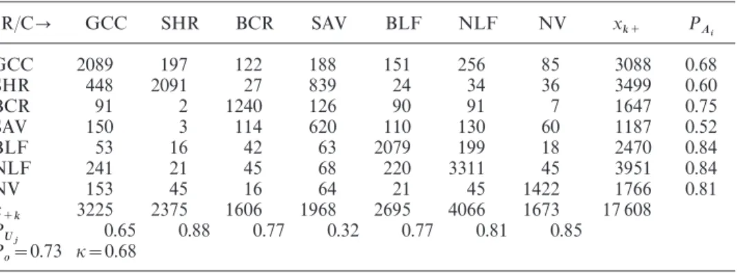
Table 3 presents cross-validated classification results for the supervised classifica-tion of the six biome classes in North America. Overall, classificaclassifica-tion accuracies (P
o) are quite good (73%), but are variable across classes. Below we summarize the results for each class.
Grasses and cereal crops (biome 1): Biome 1 generally exhibits high errors of omission with respect to the forest classes, shrublands and savannas, while omission errors for broadleaf crops are not as pronounced. Confusion is highest for the forest classes, which are structurally distinct from biome 1. The misclassification rate for biome 4 (savannas) of 6% was comparable to the misclassification rate for broadleaf forests (5%). It is likely that this result arises from the spectral properties of savannas, which possess up to 80% grass understorey. Shrubs and needleleaf forest exhibit the highest commission errors for biome 1. Shrubs contributed 14% to the total commission error (35%), and needleleaf forests contributed 7% (table 3).
Shrubs (biome 2): Background reflectance properties are a key factor influencing the variability in remotely sensed data over shrublands. Whereas shrublands in the western part of the continent have bright backgrounds, shrublands in the subarctic region are more similar to savannas in terms of their NDVI. This confusion is evident in table 3, where 13% of the grasses/cereal crops pixels and 24% of the savanna pixels contribute to a total omission error of 40%. The commission error for shrubs is generally smaller than the omission error (i.e. classes 1 and 3–6 are classified less often as shrubs than shrubs are classified as one of the other classes). Table 3. Error matrix for supervised decision tree classification of biome classes and
site-based accuracy coefficients (R, reference data; C, classified data;x+
k, column total; x k+, row total ). ER/C GCC SHR BCR SAV BLF NLF NV x k+ PAi GCC 2089 197 122 188 151 256 85 3088 0.68 SHR 448 2091 27 839 24 34 36 3499 0.60 BCR 91 2 1240 126 90 91 7 1647 0.75 SAV 150 3 114 620 110 130 60 1187 0.52 BLF 53 16 42 63 2079 199 18 2470 0.84 NLF 241 21 45 68 220 3311 45 3951 0.84 NV 153 45 16 64 21 45 1422 1766 0.81 x +k 3225 2375 1606 1968 2695 4066 1673 17 608 P Uj 0.65 0.88 0.77 0.32 0.77 0.81 0.85 P o=0.73 k=0.68
Broadleaf crops (biome 3): For broadleaf crops, table 3 shows that the highest omission errors were associated with savannas, whereas the highest commission errors were generally contributed by biome 1 (column 1 in table 3). The latter had an important influence on the proportion of the two cropland classes in the biome maps. Again, confusion between forests and broadleaf crops is more severe in terms of misclassification costs relative to confusion with biome 1.
Savannas (biome 4): The most serious source of confusion for this class arose from confusion among savannas, grasslands and cereal crops, and forests. This is clearly related to the properties of this class, which is a mixture of both grasses and trees. Also, savannas represent a small portion of the training data and were somewhat penalized by the classification algorithm.
Broadleaf forests (biome 5): Broadleaf forests had the highest P
Ai and PUj. The largest errors in this regard arose from confusion among broadleaf forests, needleleaf forests, and grasses and cereal crops. Confusion with this latter class probably arose because of the similar temporal pattern in NDVI for each of these classes. Misclassification of biome 5 as needleleaf forests is probably explained by naturally occurring mixtures of both classes.
Needleleaf forests (biome 6): The most severe sources of error for this class was the misclassification of needleleaf forests as grasses, which totals 6% (table 3). This problem could not be entirely resolved and is evident in the final biome map.
Finally, the non-vegetated class exhibited small but significant confusion with all six biome classes. In particular, biome 1 was frequently assigned to the non-vegetated class and vice versa. This is not surprising since many agricultural fields are non-vegetated and most grassland regions are senescent for a number of months each year. Some misclassification of class 7 as shrubs was also observed. Note that shrubs are defined by low vegetation density and bright backgrounds, which is similar to bare ground.
4.2. Map comparisons
In this section, an accuracy assessment of the UMD- and EDC-based six-biome maps is presented, using the training sites from the analysis presented above as reference data. The areal distribution of land cover classes from each of these maps is then compared. Error matrices are used to identify confusion among specific classes in each map.
4.2.1. Accuracy coeYcients for the UMD and EDC maps
A site-based accuracy assessment for the biome maps was performed by cross-walking the UMD and EDC maps and then overlaying the BU training sites with each. Because some sites included mixtures of classes in the EDC- and UMD-based maps, not all of the sites were used to estimate the error matrices. Specifically, the most frequent class in each map in each polygon was assigned to each site, and only those sites that were 90% covered by one biome were used. This threshold was chosen because it provided high confidence in the class label, while maintaining a sufficiently large sample in each class. Also, sites that were detected as outliers (§3.2) were not used in the error matrix. This reduced the number of sites available for the analysis. At the same time, because the sample size of 306 was still sufficiently large (Stehman 1996) and the procedures described above are designed to be conservative, the results should be relatively reliable. Note that since the SLCR map was used to cross-walk ambiguous class labels in both maps, some bias is present in the accuracy
Table 4. Error matrix and site-based accuracy coefficients for the UMD map in the biome scheme (R, reference data; C, classified data).
ER/C GCC SHR BCR SAV BLF NLF NV x k+ PAi GCC 24 3 0 5 0 2 0 34 0.71 SHR 2 5 0 0 0 0 0 7 0.71 BCR 0 0 18 0 0 0 0 18 1.00 SAV 0 0 0 5 1 0 0 6 0.83 BLF 0 1 0 1 143 5 0 150 0.95 NLF 0 0 0 1 27 39 0 67 0.58 NV 1 0 0 1 1 0 19 22 0.86 x +k 27 9 18 13 172 46 19 304 P Uj 0.89 0.56 1.00 0.38 0.83 0.85 1.00 P o=0.83 k=0.75
Table 5. Error matrix and site-based accuracy coefficients for the EDC map in the biome scheme (R, reference data; C, classified data).
ER/C GCC SHR BCR SAV BLF NLF NV x k+ PAi GCC 24 3 0 5 0 2 0 34 0.71 SHR 0 7 0 0 0 0 0 7 1.00 BCR 0 0 18 0 0 0 0 18 1.00 SAV 0 0 0 5 1 0 0 6 0.83 BLF 0 1 0 0 144 5 0 150 0.96 NLF 0 0 0 1 27 40 0 68 0.59 NV 1 1 0 1 1 0 19 23 0.83 x +k 25 12 18 12 173 47 19 306 P Uj 0.96 0.58 1.00 0.42 0.83 0.85 1.00 P o=0.84 k=0.76
coefficients. This applies particularly to broadleaf crops ( biome 3) which were cross-walked from the UMD and EDC agricultural class using the SLCR map.
Results from the analysis of the UMD-based biome scheme are shown in table 4. Overall accuracy andkare 83% and 0.75, respectively. Table 5 shows the results for the EDC map in the biome scheme. The overall accuracy was 84% andkwas 0.76. 4.3. L AI and FPAR retrievals
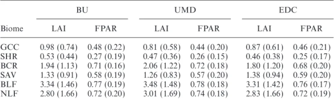
The mean and standard deviation for LAI and FPAR for each class and for each map are shown in table 6. With the exception of biome 1 (grasses and cereal crops) in the BU map, the mean and standard deviation for the three maps agree very well for both LAI and FPAR, and are in accordance with published and theoretical values (Myneniet al. 1997).
Table 7 summarizes the overall agreement (in terms of area) in LAI, FPAR and land cover classes. To generate these estimates pixels with differences smaller than 0.1 and 0.01 were considered to have the same LAI and FPAR, respectively, which slightly inflates the rate of agreement. Nonetheless, the comparison shows that agreement in LAI and FPAR are roughly 20–25% and 40–45% (respectively) greater than for land cover. This result suggests that the LAI and FPAR algorithm is relatively robust to uncertainty in land cover.
Table 6. Comparison of LAI and FPAR by mean and standard deviation (in parentheses) as a function of biome.
BU UMD EDC
Biome LAI FPAR LAI FPAR LAI FPAR
GCC 0.98 (0.74) 0.48 (0.22) 0.81 (0.58) 0.44 (0.20) 0.87 (0.61) 0.46 (0.21) SHR 0.53 (0.44) 0.27 (0.19) 0.47 (0.36) 0.26 (0.15) 0.46 (0.38) 0.25 (0.17) BCR 1.94 (1.13) 0.71 (0.16) 2.06 (1.22) 0.72 (0.18) 1.80 (1.20) 0.68 (0.20) SAV 1.33 (0.91) 0.58 (0.19) 1.26 (0.83) 0.57 (0.20) 1.38 (0.94) 0.59 (0.20) BLF 3.34 (1.46) 0.77 (0.19) 3.48 (1.48) 0.78 (0.18) 3.31 (1.42) 0.76 (0.17) NLF 2.80 (1.66) 0.72 (0.20) 3.01 (1.69) 0.74 (0.18) 2.83 (1.66) 0.72 (0.19)
Table 7. Comparison of overall agreement (in terms of area) of land cover, LAI and FPAR classes.
Map Land cover LAI FPAR
BU/UMD 42.7% 62.6% 85.6% BU/EDC 47.6% 72.5% 87.7% UMD/EDC 45.5% 81.4% 93.5%
suggest that at continental scales each of the maps appears to be capturing the distribution of each biome. However, this does not necessarily mean that there is agreement in the spatial distribution of LAI and FPAR across continental scales.
This question is addressed in tables 8 and 9, which stratify class confusions by the magnitude of LAI and FPAR differences. In table 8, the top confusion matrix shows the percentage of pixels that agree with respect to LAI (i.e.dLAI=0 where values <0.1 were set to 0), the middle matrix presents the percentage for which 0<dLAI∏1, and the bottom matrix presents the percentage of pixels whose difference was greater than 1. Similarly, table 9 presents differences in FPAR categorized according todFPAR=0, 0<dFPAR∏0.1, anddFPAR>0.1. The tables show com-parisons for the BU- and UMD-based maps only. However, these patterns (and those discussed below) were consistent between the BU and the EDC maps, and between the UMD and EDC maps.
For LAI, 62.2% of the pixels in the BU and UMD maps possessed dLAI=0. For 24.7% of the pixels 0<dLAI∏1, and 12.6% have a difference greater than 1. In this context, a substantial amount of disagreement in LAI can be attributed to confusion between biomes 1 (grasslands and cereal crops) and 4 (savannas) in the two land cover maps. Also, confusion in biomes 5 and 6 ( broadleaf forests and needleleaf forests) with biome 4 produces disagreement in LAI.
For FPAR, 85.7% of the pixels were in agreement, 9.6% have 0<dFPAR∏0.1 and 4.8% have a difference>0.1. Again, similar to the analysis of LAI, the disagree-ment in FPAR can be primarily attributed to confusion between biome 4 and biomes 1, 5 and 6. This is not too surprising since biome 4 (savannas) is defined as a mixture of classes and is characterized by a continuum of fractional vegetation cover.
5. Discussion and conclusions
The general objectives of this research were to use multi-source data to generate land cover maps in the six-biome classification scheme, to compare the resultant
Table 8. Contribution to map disagreement as a function of biome and LAI difference (in percent) for the BU and UMD maps.
UMD
EBU GCC SHR BCR SAV BLF NLF Total
dLAI=0 GCC 8.5 1.4 0.3 1.5 0.1 0.1 11.9 SHR 1.2 17.8 0.0 0.7 0.0 0.0 19.7 BCR 0.2 0.0 2.1 1.2 0.0 0.0 3.5 SAV 0.6 0.1 0.3 5.3 0.1 0.0 6.4 BLF 0.0 0.2 0.0 0.0 6.7 0.0 6.9 NLF 0.0 0.1 0.0 0.3 0.0 13.4 13.8 Total 10.5 19.6 2.7 9.0 6.9 13.5 62.2 0<dLAI∏1 GCC 0.0 0.1 0.3 3.2 0.5 1.0 5.1 SHR 0.1 0.0 0.0 1.1 0.1 0.3 1.6 BCR 0.5 0.1 0.1 1.1 0.3 0.4 2.4 SAV 1.3 0.1 0.3 0.0 0.5 0.4 2.7 BLF 0.2 0.1 0.1 0.8 0.2 0.4 1.8 NLF 1.9 0.7 0.1 2.3 0.8 5.3 11.1 Total 4.0 1.1 0.9 8.5 2.4 7.8 24.7 dLAI>1 GCC 0.0 0.0 0.0 0.1 1.9 1.2 3.2 SHR 0.0 0.0 0.0 0.0 0.3 0.6 0.9 BCR 0.0 0.0 0.0 0.0 0.8 0.7 1.5 SAV 0.0 0.0 0.0 0.0 0.4 0.3 0.7 BLF 0.2 0.0 0.3 1.1 0.0 0.4 2.0 NLF 1.0 0.1 0.1 2.1 1.0 0.0 4.3 Total 1.2 0.1 0.4 3.3 4.4 3.2 12.6
maps with existing maps at the same scale and resolution, and to assess the sensitivity of LAI and FPAR retrievals to errors in biome maps derived from remote sensing. Training data for the supervised classification algorithm were only available in the IGBP classification scheme, which is not consistent with the land surface parameteriz-ation used by radiative transfer models to retrieve LAI and FPAR from MODIS and MISR spectral reflectances. To resolve this problem, SLCR labels were used to cross-walk the training data to biome classes.
The results from this analysis point to four major conclusions. First, the decision tree algorithm implemented in this research provides a powerful technique to map biomes at continental scales using multitemporal remotely sensed data in association with ancillary data sources. However, human interaction plays a very important role at several stages of the mapping process. Second, lower accuracies were generally associated with transitional land cover types and types that occur as mixtures with other classes. In this context, it should be noted that the features used for this work (i.e. NDVI) do not necessarily represent the best metrics to characterize the structural properties of biomes, and land cover maps derived from MODIS data should significantly resolve this issue. Third, ancillary data sources (i.e. SLCR) were useful in generating the biome-based land cover maps. SLCR labels helped to reduce ambiguities in cross-walking IGBP classes to biome classes, and also provided a powerful variable for estimating decision trees for mapping biomes at continental
Table 9. Contribution to map disagreement as a function of biome and FPAR difference (in percent) for the BU and UMD maps.
UMD
EBU GCC SHR BCR SAV BLF NLF Total
dFPAR=0 GCC 8.5 1.4 0.6 4.0 1.3 0.3 16.1 SHR 1.3 17.8 0.0 1.5 0.2 0.1 20.9 BCR 0.6 0.1 2.2 2.3 1.0 0.4 6.6 SAV 1.7 0.2 0.6 5.3 0.9 0.3 9.0 BLF 0.2 0.3 0.4 1.8 6.8 0.7 10.2 NLF 0.5 0.4 0.1 1.7 1.4 18.7 22.8 Total 12.8 20.2 3.9 16.6 11.6 20.5 85.7 0<dFPAR∏0.1 GCC 0.0 0.0 0.0 0.7 1.0 0.9 2.6 SHR 0.0 0.0 0.0 0.3 0.3 0.4 1.0 BCR 0.1 0.0 0.0 0.0 0.2 0.4 0.7 SAV 0.3 0.0 0.0 0.0 0.2 0.3 0.8 BLF 0.2 0.1 0.1 0.1 0.1 0.1 0.7 NLF 1.4 0.3 0.1 1.9 0.2 0.0 3.9 Total 2.0 0.4 0.2 3.0 2.0 2.1 9.6 dFPAR>0.1 GCC 0.0 0.0 0.0 0.0 0.2 1.1 1.3 SHR 0.0 0.0 0.0 0.0 0.0 0.4 0.4 BCR 0.0 0.0 0.0 0.0 0.0 0.3 0.3 SAV 0.0 0.0 0.0 0.0 0.0 0.2 0.2 BLF 0.0 0.0 0.0 0.0 0.0 0.1 0.1 NLF 1.0 0.2 0.0 1.1 0.2 0.0 2.5 Total 1.0 0.2 0.0 1.1 0.4 2.1 4.8
scales. Finally, retrievals of LAI and FPAR proved to be relatively robust to uncertainty in land cover.
In addition to these general conclusions, additional lessons were learned in the mapping process. In particular, exploratory data analysis involving the detection of multivariate outliers in the training data is a crucial step. Even though the effect of removing outliers is not directly reflected in the overall accuracy coefficients, class-specific misclassifications were reduced. For this analysis, removal of outliers was performed interactively in a manual fashion. For operational mapping of global land cover this process needs to be automated in a rigorous and robust fashion.
It should also be noted that shortcomings in the sampling design will affect accuracy statistics derived from the training data (Congalton 1991, Stehman 1996). In this context, the sample of training sites used for this work is biased in three ways. First, SLCR labels were used to cross-walk the IGBP labels in the training data to biome labels. Secondly, generation of supplemental training sites used the SLCR map as a guideline for developing a stratified sampling scheme. Thirdly, SLCR labels were used as a feature in the estimation of the tree. As a result, each of the six-biome maps is biased (in varying degrees) towards the information content of the SLCR map.
Unfortunately, few alternative sources are available that map actual land cover (as opposed to potential vegetation) at continental scales that could serve as a basis for stratifying North America into different sampling units. This problem is further
complicated by the expense of generating a statistically sound training site dataset at continental and global scales. The accuracies reported here are therefore expected to contain some bias. However, because the sample size is large, the results should be reliable. Issues relating to shortcomings in the sampling scheme and uncertainties in the training database are not addressed in this work and are the subject of future research.
Further inspection of table 2 shows that a wide spectrum of naturally occurring vegetation is not captured by the six-biome classification scheme. In particular, the definition of fractional cover is not consistent. For example, broadleaf forests and needleleaf forests are defined by ground cover greater than 70%, whereas savannas are defined by less than 20% overstorey. A significant amount of naturally occurring land cover, however, falls in the category of 20–70% ground cover (DeFries et al. 2000). This caused problems cross-walking the IGBP classes to biomes, and the use of the SLCR-to-biome LUT only partially resolved this issue. This problem is reflected in the accuracy statistics for savannas.
The sensitivity analysis for the LAI and FPAR retrievals showed that disagree-ment, and consequently uncertainty, in land cover maps do not necessarily translate into strong disagreement in resultant maps of LAI and FPAR. The areas in the LAI and FPAR maps that showed disagreement relate primarily to biome 4 (savannas), which may be related to the way that this class is defined. Specifically, pixels that possess substantial levels of heterogeneity are assigned to one of six uniform biome classes. This translates into disagreement between savannas and other related classes, most likely needleleaf and broadleaf forests and grasslands. At the same time, compar-ison of retrieved LAI values for pixels belonging to biome 1 in one map and biome 4, 5 or 6 in the other map, showed that the associated LAI values were consistently low. Therefore confusion between these classes does not cause major errors in retrievals of LAI or FPAR. The effects of class heterogeneity and subpixel mixtures on LAI and FPAR retrievals at different spatial scales has recently been explored by Tianet al. (2002).
It is important to note that the decision tree classification used a 1 year time series of NDVI to discriminate the biome classes. Even though time series of NDVI have been widely used for the purpose of land cover classification (Lovelandet al. 1995, Friedlet al.2000b), it can be argued that a classification based solely on the temporal trajectory of NDVI may not be sufficient to differentiate land cover types. This is particularly true for the six biomes considered here, which are defined by structural properties rather than phenological attributes. As a consequence, it is reasonable to consider additional metrics in the classification process that might better account for the structural properties of biomes. The spectral and directional information from new instruments such as MODIS and MISR may therefore provide a means to improve classification accuracies with respect to biomes.
Acknowledgments
This work was supported by NASA Grant NAG5-7218 and contract NAS5-96 061. The hard work of the land cover team at BU is gratefully acknowledged along with the staffof the Global Land 1 km AVHRR project at EROS Data Center who kindly provided the 1 km AVHRR data.
References
B, W.,P, T., andS, V., 1998, Prelaunch characteristics of the Moderate Resolution Imaging Spectroradiometer (MODIS) on EOS-AM1.IEEE T ransactions on Geoscience and Remote Sensing,36, 1088–1100.
B, L., F, J., O, R., and S, C., 1984, Classification and Regression T rees(Belmont, CA: Wadsworth International Group).
C, G.,G, S., M, N., R, J., andR, D., 1992, Fuzzy ARTMAP: a neural network architecture for incremental supervised learning of analog multidimensional maps.IEEE T ransactions on Neural Networks,3, 698–713.
C, J.,L, H.,C, Z.,P, H., andH, F., 1997, Multitemporal, multichannel AVHRR datasets for land biosphere studies—artifacts and corrections.Remote Sensing of Environment,60, 35–37.
C, J., 1960, A coefficient of agreement for nominal scales.Educational and Psychological Measurement,20, 37–46.
C, R., 1988, Using spatial autocorrelation analysis to explore the errors in maps generated from remotely sensed data. Photogrammetric Engineering and Remote Sensing,54, 587–592.
C, R., 1991, A review of assessing the accuracy of classifications of remotely sensed data.Remote Sensing of Environment,37, 35–46.
DF,R., and T, J., 1994, NDVI-derived land cover classifications at a global scale.International Journal of Remote Sensing,15, 3567–3586.
DF,R.,H, M.,T, J., andS, R., 1998, Global land cover classi-fication at 8 km spatial resolution: the use of training data derived from Landsat imagery in decision tree classifiers. International Journal of Remote Sensing, 19, 3141–3168.
DF,R.,H, M., andT, J., 2000, Continuous fields of vegetation character-istics: a linear mixture model applied to multi-year 8 km AVHRR data.International Journal of Remote Sensing,21, 1389–1414.
D, R., andH-S, A., 1988, Modeling deforestation: a study of GCM land-surface parameterization.Quarterly Journal of the Royal Meteorological Society, 114, 439–462.
F, M. A., andB, C., 1997, Decision tree classification of land cover from remotely sensed data.Remote Sensing of Environment,61, 399–409.
F, M. A., B, C., and S, A., 1999, Maximizing land cover classification accuracies produced by decision trees at continental to global scales. IEEE T ransactions on Geoscience and Remote Sensing,27, 969–977.
F, M. A., W, C., G, S., M, D., S, A. H., and B -S, C., 2000a, A note on procedures used for accuracy assessment in land cover maps derived from AVHRR data. International Journal of Remote Sensing, 21, 1073–1077.
F, M. A.,M, D.,MI,D.,G, F.,H, J. F. C., andS, A. H., 2000b, Characterization of North American land cover from NOAA-AVHRR data using the EOS MODIS land cover classification algorithm. Geophysical Research L etters,27, 977–980.
G, S., andW, C., 1996, Remote sensing of forest change using artificial neural networks.IEEE T ransactions on Geoscience and Remote Sensing,34, 398–404. H, M.,DF, R.,T, J., andS, R., 2000, Global land cover
classi-fication at 1 km spatial resolution using a classiclassi-fication tree approach.International Journal of Remote Sensing,21, 1331–1364.
H, T.,T, R., andF, J., 2001,T he Elements of Statistical L earning: Data Mining, Inference, and Prediction(New York: Springer-Verlag).
H, S., 1993, Neural networks: a comprehensive foundation (Upper Saddle River, New Jersey: Prentice Hall ).
J, C.,T, J.,H, B., andT, C., 1985, Analysis of the phenology of global vegetation using meteorological satellite data.International Journal of Remote Sensing,6, 1271–1318.
J, C., H, D., S, V., P, J., R, G., S, A., L, W., M, R.,K, Y.,R, S.,N, R.,V, E.,T, J., DF, R.,R, D.,W, Z.,H, A., vanL, W.,W, R.,G, L., M, J.-P.,L, P., andB, M., 1998, The Moderate Resolution Imaging Spectroradiometer (MODIS): land remote sensing for global change research. IEEE T ransactions on Geoscience and Remote Sensing,36, 1228–1249.
K, Y.,M, J.,D, D.,M, R., andR, S., 1998a, Synergistic algorithm for estimating vegetation canopy leaf area index and fraction of absorbed photosynthetically active radiation from MODIS and MISR data. Journal of Geophysical Research,103, 32257–32275.
K, Y., M, J., D, D., M, R., V, M., P, B., and G, N., 1998b, Estimation of vegetation canopy leaf area index and fraction of absorbed photosynthetically active radiation from atmosphere-corrected MISR data. Journal of Geophysical Research,103, 32239–32256.
L, J., and W, D., 1989, Simulation of the regional climatic impact of Amazon deforestation.Nature,342, 411–413.
L, T., and B, A., 1997, The IGBP-DIS global 1 km land cover data set, DISCover: first results.International Journal of Remote Sensing,18, 3289–3295. L, T. R.,M, J. W.,O, D. O., andB, J. F., 1991, Development of
a land cover characteristics data base for the conterminous U.S. Photogrammetric Engineering and Remote Sensing,57, 1453–1463.
L, T. R.,M, J. W.,B, J. F.,O, D. O.,R, B. C.,O, P., and H, J., 1995, Seasonal land cover of the United States. Annals of the Association of American Geographers,85, 339–355.
L, T. R.,Z, Z.,O, D. O.,B, J. F.,R, B. C., andY, L., 2000, An analysis of the IGBP global land-cover characterization process. Photogrammetric Engineering and Remote Sensing,65, 1021–1031.
M, J., 1989, An empirical comparison of pruning methods for decision tree induction. Machine L earning,4, 227–243.
M, A., andS, A., 1994, Characteristics of composited AVHRR data and problems in their classification.International Journal of Remote Sensing,15, 3473–3491. M, D., S, A., H, J., and LC, J., 1999, The IGBP DISCover
confidence sites and the system for terrestrial ecosystem parameterization: tools for validating global land-cover data.Photogrammetric Engineering and Remote Sensing, 65, 1061–1067.
M, R. B.,M, S.,I, J.,P, J.,G, N.,P, B.,V, M.,K, D., andW, D., 1995, Optical remote sensing of vegetation: modeling, caveats and algorithms.Remote Sensing of Environment,51, 169–188.
M, R. B.,N, R., andR, S., 1997, Estimation of global leaf area index and absorbed PAR using radiative transfer models.IEEE T ransactions on Geoscience and Remote Sensing,35, 1380–1393.
Q, J., 1987, Simplifying decision trees.International Journal of Man–Machine Studies, 27, 221–234.
Q, J., 1993,C4.5: Programs for Machine L earning(San Mateo, CA: Morgan Kaufmann). Q, J., 1996, Bagging, boosting, and C4.5. Proceedings of the T hirteenth National
Conference on Artificial Intelligence(Portland, OR: AAAI Press), pp. 725–730. R, F., 1975, Generalization of the gap test for the detection of multivariate outliers.
Biometrics,31, 93–101.
R, G., andF-L, K., 1986, A coefficient of agreement as a measure of thematic classification accuracy. Photogrammetric Engineering and Remote Sensing, 52, 223–227.
R, S.,J, C.,S, V.,H, D.,B, J.,K, Y.,S, A.,H, A.,V, J. M. V.,W, Z.,T, P., andC, D., 1994, Terrestrial remote sensing science and algorithms planned for EOS/MODIS. International Journal of Remote Sensing,15, 3587–3620.
R, S. W.,L, T. R.,P, L. L.,N, R. R., andH, E. R.J,1995, A remote sensing based vegetation classification logic for global land cover analysis. Remote Sensing of Environment,51, 39–48.
S, S. R., andL, D., 1991, A survey of decision tree classifier methodology. IEEE T ransactions on Systems, Man, and Cybernetics,21, 660–674.
S, R., 1997, Remote Sensing, Models and Methods for Image Processing (San Diego: Academic Press).
S, R., 1990, The strength of weak learnability.Machine L earning,5, 197–227.
S, S., 1996, Estimating the Kappa coefficient and its variance under stratified random sampling.Photogrammetric Engineering and Remote Sensing,62, 401–402.
S, M., 1977, Asymptotics for and against cross-validation.Biometrika,64, 29–35. S, A.,M, D.,B, J.,F, G.,F, M.,G, S.,H, J.,L,
E., MI, D., M, A., S, C., and W, C., 1999, MODIS L and Cover Product Algorithm T heoretical Basis Document (AT BD), Version 5.0. Boston University Center for Remote Sensing, Boston, MA.
T, Y., W, Y., Z, Y., K, Y., B, J., and M, R. B., 2002, Radiative transfer based scaling of LAI/FPAR retrievals from reflectance data of different resolutions.Remote Sensing of Environment, in press.
T, J.,J, C.,L, W.,G, C., andMM,J., 1991, Global land cover classification by remote sensing: present capabilities and future possibilities.Remote Sensing of Environment,35, 243–255.
Z, Z., andY, L., 1996, Characteristics of the 1-km AVHRR data set for North America. International Journal of Remote Sensing,17, 1915–1924.