1
Multi-objective Optimal Design of Friction Stir Welding Considering
Quality and Cost Issues
Qian Zhang1*, Mahdi Mahfouf2, George Panoutsos2, Kathryn Beamish3 and Xiaoxiao Liu4
1School of Engineering and Digital Arts, University of Kent, Canterbury, Kent, CT2 7NT, UK
Email: [email protected] Tel: +44 (0)1227 827083
2Department of Automatic Control and Systems Engineering, The University of Sheffield,
Sheffield, S1 3JD, UK.
3TWI Ltd, Great Abington, Cambridge, CB1 6AL, UK.
4Department of Mechanical Engineering, The University of Sheffield, Sheffield, S1 3JD, UK. *Corresponding author
Abstract
Because of the high complexity in microstructure evolution in friction stir welding, it becomes very difficult to design optimal welding parameters. To solve this problem, in the current paper, soft-computing-based data-driven models are developed to provide accurate and instant predictions for the welding process, and a multi-objective optimisation approach is employed to find optimal solutions to achieve the desired quality and economic objectives. The current work studies the aluminium AA5083-O as an example, where not only weld quality and mechanical properties of a joint, but also in-process properties and production cost, are considered as objectives in the optimal design.
Keywords
welding; aluminium; cost; properties; multi-objective; optimisation; design
1. Introduction
Friction Stir Welding (FSW) has been shown to be a very practical joining technique for various industrial problems in aerospace, railway, shipbuilding, etc. A general FSW process involves severe plastic deformation in a high-temperature environment and produces good micro-structural and mechanical properties for the post-weld materials. From the viewpoint of application, it is essential to generate predictive models for internal process features and as-weld properties, and then utilise them to design effective welding conditions to produce structurally sound, defect-free and low-cost welds. The conventional approach of designing welding conditions is often a time-consuming trial-and-error process and is almost impossible
2 to find the ‘optimal’ solutions. The high complexity of FSW, caused by the complex thermo-mechanical processes and intense plastic deformation, makes the design even more difficult. In order to achieve the optimal design of welding parameters in a fast, accurate and cost-effective way, one may employ the soft computing techniques into the relevant empirical modelling and optimisation procedures.
In recent years, multi-objective optimisation algorithms based on soft-computing principles have been gradually applied into materials and manufacturing processes1-5. In the review article6, Tutum and Hattel have foreseen a bright perspective of implementing soft-computing-based optimisation approaches into the FSW design and suggested some practical directions for the future research. However, only few works have been carried out in this area. Tansel et al.7 employed a Genetic Algorithm (GA) to find the best operating conditions from the developed Artificial Neural Network (ANN) models. In Roshan et al.’s paper8, a Neuro-Fuzzy System was applied for predicting the mechanical properties of the aluminium AA7075 and a simulated annealing algorithm was further used to exploit the models to achieve optimal characteristics. Parida and Pal9 proposed a fuzzy-assisted Taguchi approach
to optimise multiple process parameters of FSW, in which the multi-objective optimisation problem was strategically converted into an equivalent single objective optimisation case. In the studies10,11, a multi-objective Genetic Algorithm NSGA-II was used into thermal models to solve two-objective optimisation problems, i.e. minimising the peak residual stress in a weld and maximising welding speed simultaneously10, and maximising tool life and production efficiency simultaneously11. In Shojaeefard et al.’s paper12, the authors used the Multi-objective Particle Swarm Optimisation (MOPSO) to find the process conditions to reach the optimal design of mechanical properties. The above researches considered either single-objective7-9 or two-objective10-12 optimal designs. In this paper, more than two conflicting optimisation objectives are taken into consideration, which include not only mechanical properties but also weld quality, in-process attributes and economic cost of welding.
2. Materials and Experiments
In this work, the study focuses on a frequently-used non-heat-treatable aluminium alloy AA5083-O, which possesses high strength, good formability and excellent resistance to corrosion13. In the experiments, the 5.8mm-thick AA5083-O plates were welded as butt
3 welds. A well-designed second-generation tool MX-TrifluteTM, in conjunction with a 25 mm diameter scroll shoulder14, was used in welding. Such a FSW tool has been proven to be very successful, as it improves the material flow thereby enables a significant increase of the maximum achievable welding speed15.
Two attributes used for the control of FSW are the tool rotation speed (rpm) and the forward movement step along the joint line (representing welding speed) (mm rev-1). All the experimental trials were undertaken based on a 5-by-5 parameter test matrix, which includes five levels of tool rotation speeds, i.e. 280, 355, 430, 505 and 580 rpm, and five levels of forward feed rates, i.e. 0.6, 0.8, 1.0, 1.2 and 1.4 mm rev-1.
A new revolutionary on-line sensory platform named Advanced Rotating Tool Environment Monitoring and Information System (Artemis), which is a rotating tool holder that is extensively instrumented, was developed by TWI. It can in-process collect and log data relating to the internal status of welding, as shown in Figure 1, including various temperatures of different parts, such as the tool temperature and the shaft temperature, torque and various forces on the tool, such as the axial compression, the lateral bending force and the traverse force.
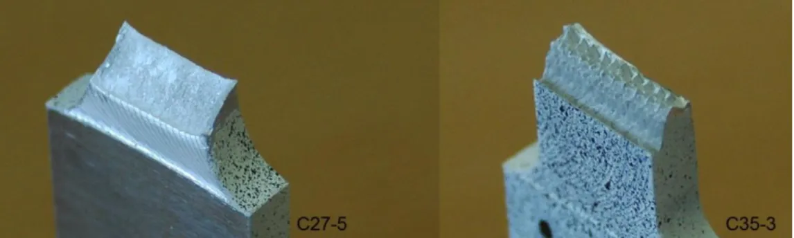
For all the welds, tensile tests were accomplished at the room temperature, from which elongation, reduction of area, yield strength and ultimate tensile strength were derived. They utilised the Digital Image Correlation (DIC) technique, a LaVision two-dimensional system with a monochrome camera of 2 Megapixel, to measure displacement and collect data. For every set of welding conditions, 5 separate specimens in 2 geometries were produced and tested. They were all machined in the transverse direction. In such transverse tensile tests, the measured strength relates to the weakest area of the weld while the obtained ductility represents the mean situation across different zones. Two types of failure in these tensile tests can be observed, as shown in Figure 2. The first is a shear fracture occurred in the heat-affected zone, which has a lower strength because of the generation of heavily-coarsened precipitates and non-precipitate regions16. For those joints including defects, the second type of failure happened in the nugget region, where voids had formed.
For a friction stirred weld, the general defects are flow-related volumetric defects17, where materials are not stirred and mixed adequately. In details, when the tool is rotating and
4 gradually moving forward, the material softened around the tool pin will be forced to transfer from the advancing side to the retreating side along the front path of the tool, therefore a void will occur at the advancing side. If the material flow coming back from the retreating side along the back of the tool cannot fill the vacated area fully and instantaneously, the volumetric defects will happen18.
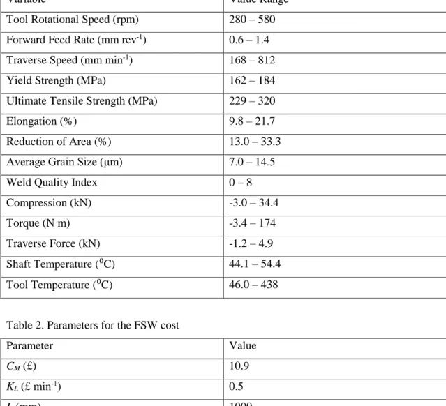
To evaluate the weld quality, four separate tests were carried out, i.e. a surface inspection, a cross-section inspection, a surface bend test and a root bend test. For each single test, a sub-index with a value ranging from 0 to 3 is used to express the weld quality degree. In order to represent the overall status of weld quality, four sub-indices are summed together to form an integral weld quality index with its value ranging from 0 to 12, where 0 means excellent quality and 12 means complete failure in welding. The data ranges of welding parameters, internal process variables, mechanical properties and weld quality index are summarised in Table 1.
3. Cost of Production
Generally, the cost of welding a piece of materials using FSW consists of four main parts as follows:
𝐶𝑈 = 𝐶𝑀+ 𝐶𝐿+ 𝐶𝐸+ 𝐶𝑇 (1)
where CU (£) represents the overall unit cost (overall cost of each piece); CM (£) represents
the unit material cost, which is fixed in this study due to the same material and the same geometry used; CL (£), CE (£) and CT (£) are respectively the labour cost, energy cost and tool
wear cost for producing a single piece.
The labour cost is expressed as follows:
𝐶𝐿 = 𝐾𝐿𝑡𝑤 = 𝐾𝐿𝑣𝐿
𝑤 (2)
where KL (£ min-1) is the unit labour cost; tw (min) represents the unit welding time; L (mm)
represents the length of the work pieces, and vw (mm min-1) is the welding speed. Similar to
above, the energy (electricity) cost per piece is as follows:
𝐶𝐸 = 𝐾𝐸𝑃𝑤𝑡𝑤 = 𝐾𝐸𝑃𝑤𝑣𝐿
𝑤 (3)
where KE (£ kWh-1) is the electricity cost per kWh; Pw (kW) represents the power of the
5 The cost relating to tool wear can be expressed as follows:
𝐶𝑇 = 𝐾𝑇𝑡𝑇𝑤 = 𝐾𝑇𝑣𝐿
𝑤𝑇 (4)
where KT (£) represents the value of the welding tool; T (min) is its tool life. Assuming the
Taylor equation for tool life19 is applicable in this case:
𝜋𝐷𝑣𝑟𝑇𝑛 = 𝐾 (5)
where D (mm) represents the diameter of the tool pin, vr (rpm) represents the rotational speed
of the tool; K and n are constants in a particular welding tool.
Therefore, the overall unit cost is expressed in the following form:
𝐶𝑈 = 𝐶𝑀+ 𝐶𝐿+ 𝐶𝐸+ 𝐶𝑇 = 𝐶𝑀+ (𝐾𝐿 + 𝐾𝐸𝑃𝑤)𝑣𝐿
𝑤+ 𝐾𝑇
𝐿(𝜋𝐷𝑣𝑟)1/𝑛
𝑣𝑤𝐾1/𝑛 (6)
The parameters relating to the cost of welding are summarised in Table 2. Some of them are approximate values, but can be adopted in experiments without any loss of generality.
4. Predictive Models
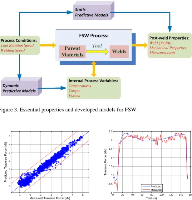
Figure 3 illustrates different groups of attributes in the FSW process, i.e. process conditions, in-process variables and post-weld properties. Both of the internal and post-weld properties are important, as the former can provide rich but sometimes hidden information about the undergoing process and the latter represent the quality of the final product. Due to the severe plastic deformation and the complex recrystallization phenomena in FSW, it is very complicated and difficult to derive suitable analytical models to predict these properties.
The previous study20,21 has successfully employed the data-driven modelling techniques to construct a number of reliable predictive models for various post-weld properties, relating to microstructure, weld quality, and mechanical properties. The modelling method was designed based on fuzzy rule-based systems22,23, which are very practical to be applied into the nonlinear, data-driven leaning context. An improved version of the data-driven fuzzy modelling approach, with a representative data selection method, was further implemented to develop dynamic models for predicting internal process attributes24, as demonstrated in Figure 3. Such dynamic models can predict the internal process features at various time points during the whole welding process. Figure 4(a) demonstrates the prediction performance of one elicited traverse force model (with 100 fuzzy rules, RMSE = 0.2501 and correlation coefficient r = 0.9820). Figure 4(b) demonstrates its validation in the real-time application, where the model is successfully used to predict the changing of the traverse force
6 during welding for a certain set of welding conditions. Such models are considered to be robust, as they always provide moderate predictions and neglect the disturbances and noises involved in the learning examples.
5. Multi-objective Optimal Design
The optimal design of the welding process is naturally a multi-objective problem, in which the desired objectives can conflict with each other, for example, strength and ductility may be a pair of conflicting objectives, and weld quality and production cost may also conflict as objectives. In this study, we employed a novel nature-inspired algorithm, i.e. the multi-objective Reduced Space Searching optimisation (MO-RSSA)25,26. It is an optimisation and search technique motivated by the human behaviour of searching for the best solution in their daily life. Normally, if one seeks for a target without any preliminary knowledge, common sense leads to scan a relatively large area initially; should one obtains some clues indicating the suspicious areas, the search region is then justifiably decreased for more complete inspection. Conversely, if one appears to be trapped in a worthless space, then the field of vision should be expanded to look for fresh clues. Based on this idea, a simple operator RSSA was designed that can shift the search space and change its scale.
To extend the algorithm to cope with multi-objective instances, the varying weighted aggregation strategy27 was employed and an extra archive was designed to record the observed Pareto-optimal solutions. Most of the recent multi-objective optimisation algorithms were designed based on the Pareto-dominance population, which generally possess well-distributed solutions. However, some research showed that the Pareto-dominance-based algorithm may find difficulties when dealing with the problems with a large number of objectives. The presence of all non-dominated solutions in the population may ease the selection pressure and cannot push the population enough towards the optimal region28. The varying-weighted-aggregation-based algorithm is relatively straightforward and computationally efficient. It enables the solutions to quickly converge to the relatively ‘good’ searching areas and also appears very practical in finding the ‘knee’ region29 out of a Pareto front. The algorithm MO-RSSA has been tested using some challenging benchmark testing problems, ZDT series and DTLZ series problems, and shown to perform better than some well-known algorithms, such as SPEA2 and NSGA-II26. For the experiments in the following section, the parameter configuration was set as shown in Table 3 without any loss of generality. The experimental results show that these parameter settings are robust and work
7 well across all the experiments.
6. Results and Discussion
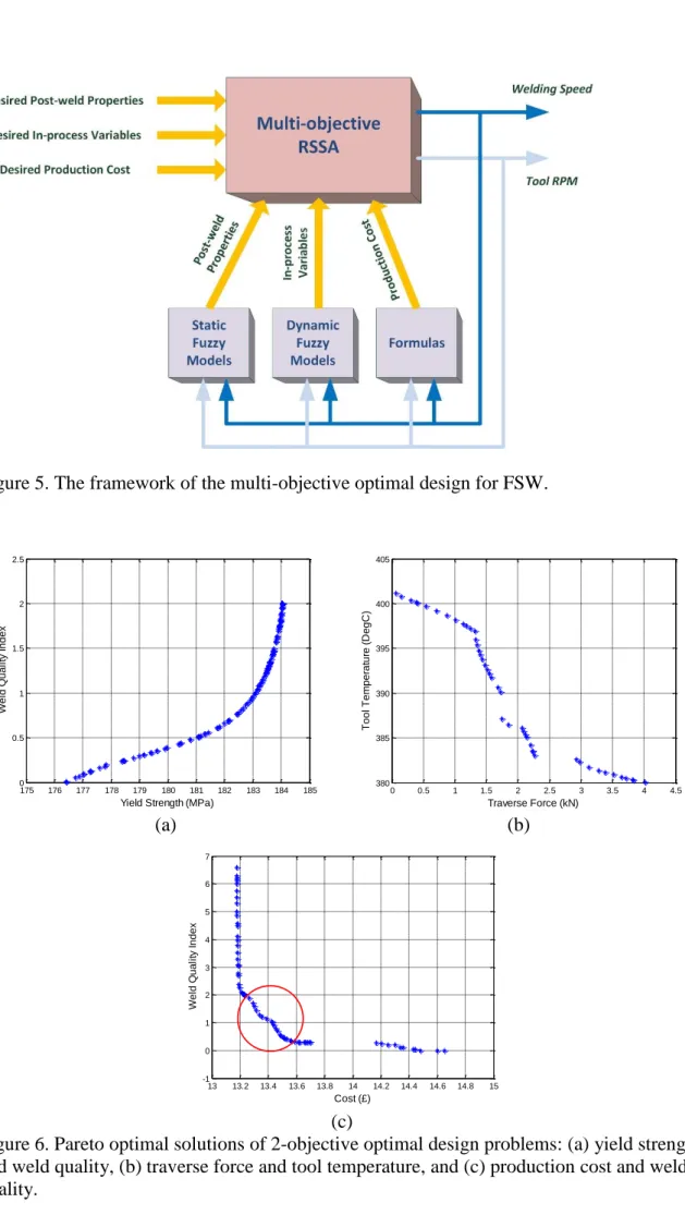
Figure 5 illustrates the framework of the multi-objective optimal design for FSW. For every single case of the following experiments, 10 runs were carried out and the set of results in an ‘average’ performance are shown and discussed as examples. It is found that the results in different runs are very consistent.
In the first experiment, we aim to maximise the mechanical property, yield strength, as well as the weld quality. The objective functions used into the optimisation algorithm can be defined as follows:
Objective 1: maximise YS (x) Objective 2: minimise WQ (x)
where YS (x) and WQ (x) are the yield strength and weld quality index variables, respectively;
x is the process condition vector including the tool rotation speed and forward feed rate.
Figure 6(a) shows one group of the Multi-objective optimal solutions in a 2-objective plane. To show more details, ten solutions out of the whole solution set are selected and listed in Table 4. The results are shown to be of low tool rotation speeds and relatively high forward feed rates. Such observation accords with the general recrystallization principles30, as the low heat input, caused by a low rotation speed and a high forward feed speed, leads to the generation of fine grains, which always relates to high yield strength. However, the high forward feed rate will also worsen the weld quality, as the void defect may form due to the insufficient material flow. In application, one may choose the welding conditions close to 280 rpm tool rotational speed and 1.3 mm/rev feed rate, which guarantees an excellent weld quality and a relatively strong yield strength, 181 MPa out of the range of 162 ~ 184 MPa.
In the second experiment, the traverse force and tool temperature profile during the welding process were considered as objectives, where one would like to minimise the traverse force to avoid tool breakage and maintain the tool temperature at a certain level to achieve the desired microstructure. In this case, the objective functions can be designed as follows:
8 Objective 2: minimise ∑𝑝𝑖=1(𝑇𝑇(𝒙, 𝑡𝑖) − 𝑇𝑇𝑡𝑎𝑟𝑔𝑒𝑡)2⁄𝑝
where TF (x, ti) and TT (x, ti) are respectively the traverse force and tool temperature
variables, ti (i = 1, 2, …, p) are the time points in the welding process, p is the sample size;
TTtarget is the value of the target tool temperature. In this experiment, TTtarget is set to be 380
⁰C.
Figure 6(b) shows the optimal solutions in their objective space. For details, ten out of all are chosen and shown in Table 5. From the table, it can be observed that a faster welding speed (the product of the tool rotation speed and the forward feed rate) brings higher traverse resistance but lower tool temperature, because a faster welding speed decreases the welding time and thus decrease the heat generation. For the practitioners who prioritise to protect the tool, they can utilise a solution with a low tool rotational speed (280 ~ 300 rpm) and a high forward feed rate (1.2 ~ 1.4 mm/rev). Such a solution will ease the pressure on the tool to avoid the unexpected breakage and extend the tool-life, and at the same time it leads to a tool temperature (around 395 ⁰C) that is close to the target one (380 ⁰C).
The third design problem aims to simultaneously minimise the cost of production and weld quality. The objective functions are defined as follows:
Objective 1: minimise Cost (x) Objective 2: minimise WQ (x)
where Cost (x) is the production cost variable calculated using Equation (6).
Figure 6(c) includes the obtained non-dominated solutions and ten of them are chosen as examples to show in Table 6. The solutions with the lowest cost of production are those implementing high welding speed (high tool rotational speed and high forward feed rate), which can greatly shorten the welding time for a single joint, and therefore reduce the labour cost and energy cost. Although the tool wear cost is increased a little by an increasing welding speed, it is only a minor factor if compared with the labour cost and energy cost. For the FSW of the aluminium, one tool can last for thousands of meters of welding. However, fast welding speed often causes the formulation of void flaws due to the insufficient material flow. In Figure 6(c), one can observe a ‘knee’ region in the Pareto front, out of which a solution will lose significantly in one objective without much gain in other objectives. From the viewpoint of multi-criteria decision making29, it is best to utilise the solutions within the
9 ‘knee’ region. For instance, the 4th solution (507 rpm tool rotational speed and 1.29 mm/rev forward feed rate) in Table 6 is a good choice in consideration of application. Under this welding condition, one can achieve very good weld quality (weld quality index < 1) and maintain a very low production cost (unit cost £13.32). As the average unit production cost without optimal design is £16.4, the generated solution contributes to a big save of £3.08 per unit, which is 18.8% of the total cost.
In the fourth design problem, we consider the following three objectives: Objective 1: maximise YS (x)
Objective 2: minimise WQ (x) Objective 3: minimise Cost (x)
Figure 7 shows the Pareto-optimal solutions in 3-D and 2-D objective spaces and Table 7 gives ten solutions out of all. From Figure 7, one can clearly observe the trade-off among different objectives. For example, the solutions with better weld quality (lower weld quality index value) generally have lower yield strength, while the solutions with higher yield strength generally have worse weld quality (higher weld quality index value). If the users prefer to have the perfect weld quality, they may choose the designs with a relatively fast tool rotation speed and a relatively low feed forward rate. If the users are more concerned with production cost or yield strength, they could employ the designs with a higher feed forward rate. Under a ‘moderate’ solution (295 rpm tool rotational speed and 1.34 mm/rev feed rate), one can achieve a strong yield strength (more than 180 MPa) and a relatively low cost (around £14.5), while maintain a good weld quality, where the weld quality index is less than 1. In the first experiment where only the yield strength and the weld quality were considered as objectives, we have obtained some decent solutions (280 rpm tool rotational speed and 1.3 mm/rev feed rate). However, their production cost is £0.5 higher than the current solutions where the cost is considered as an extra objective.
The fifth design considers the following five-objective optimal problem: Objective 1: maximise YS (x)
Objective 2: minimise WQ (x)
Objective 3: minimise ∑𝑝𝑖=1𝑇𝐹(𝒙, 𝑡𝑖)⁄𝑝
Objective 4: minimise ∑𝑝𝑖=1(𝑇𝑇(𝒙, 𝑡𝑖) − 𝑇𝑇𝑡𝑎𝑟𝑔𝑒𝑡)2⁄𝑝 Objective 5: minimise Cost (x)
10 Figure 8 displays the Pareto-optimal solutions in 3-D and 2-D plots and Table 8 shows ten examples of the solutions. From Figure 8, one can find some intricate relationships among different objectives. For example, with the increase of the welding speed, the average tool temperature is normally decreasing due to less heat generated; however, the cost of production may be either increasing or decreasing depending on different situations. If the labour cost and energy cost play a major role, the overall cost will decrease due to the short welding time; if the tool wear cost becomes a major factor, the overall cost may increase when higher tool rotation speed is applied. It can be observed that the optimisation algorithm is capable to generate a set of well-spread Pareto-optional solutions close to these predefined objectives, which provide practitioners diverse solutions for the FSW design. From an application point of view, a solution like the 7th solution in Table 8 provides a good compromise between various objectives. Under such welding conditions, one can achieve good yield strength (176 MPa) and good weld quality (weld quality index 0.90). The traverse force (2.49 kN) is acceptable and the tool temperature (397 ⁰C) is not far from the target (380
⁰C). Most importantly, such welding conditions relate to a very low production cost (unit cost £13.67). Compared with the average unit production cost without optimal design (£16.4), this solution contributes to a big save of £2.73 per unit (16.6% of the total cost). It is also worth noting that, for a single FSW machine working with its full load, such optimal designs may save tens of thousands pounds per annual in the production cost, which highlights the merit of the optimal design.
7. Conclusions
In this paper, multi-objective optimal designs have been carried out to find the best process conditions for friction stir welding, based on the developed predictive models. In details, a multi-objective optimisation algorithm, the multi-objective Reduced Space Searching optimisation, has been successfully applied into a series of 2-objective to 5-objective optimal design problems, where both quality and cost aspects have been considered. A range of well-distributed ‘Pareto-optimal’ solutions have been found, which are close to the desired objectives and have shown good consistency with the general understanding about friction stir welding in its physical and economic behaviours. The results can help the users understand the overall trends of gain and sacrifice. By implementing a suitable design among the competitive choices, a manufacturer is able to achieve the best in welding productivity, process reliability and cost efficiency.
11
References:
1. N. Chakraborti: ‘Critical assessment 3: the unique contributions of multi-objective evolutionary and genetic algorithms in materials research’, Mater. Sci. Technol., 2014, 30, (11), 1259-1262.
2. W. Paszkowicz: ‘Genetic algorithms, a nature-inspired tool: a survey of applications in materials science and related fields: part II”, Mater. Manuf. Processes, 2013, 28, (7), 708-725. 3. S. Datta, Q. Zhang, N. Sultana and M. Mahfouf: ‘Optimal design of titanium alloys for prosthetic applications using a multi-objective based genetic algorithm’, Mater. Manuf. Processes, 2013, 28, (7), 741-745.
4. Q. Zhang, M. Mahfouf, J. R. Yates, C. Pinna, G. Panoutsos, S. Boumaiza, R. J. Greene and L. de Leon: ‘Modeling and optimal design of machining-induced residual stresses in aluminium alloys using a fast hierarchical multiobjective optimization algorithm’, Mater. Manuf. Processes, 2011, 26, (3), 508-520.
5. Q. Zhang and M. Mahfouf: ‘A modified PSO with a dynamically varying population and its application to the multi-objective optimal design of alloy steels’, Proc. 2009 IEEE Cong. on ‘Evolutionary Computation’, Trondheim, Norway, 2009, IEEE, 3241-3248.
6. C. C. Tutum and J. H. Hattel: ‘Numerical optimisation of friction stir welding: review of future challenges’, Sci. Technol. Weld. Join., 2011, 16, (4), 318-324.
7. I. N. Tansel, M. Demetgul, H. Okuyucu and A. Yapici: ‘Optimizations of friction stir welding of aluminum alloy by using genetically optimized neural network’, Int. J. Adv. Manuf. Technol., 2010, 48, 95–101.
8. S. B. Roshan, M. B. Jooibari, R. Teimouri, G. Asgharzadeh-Ahmadi, M. Falahati-Naghibi and H. Sohrabpoor: ‘Optimization of friction stir welding process of AA7075 aluminum alloy to achieve desirable mechanical properties using ANFIS models and simulated annealing algorithm’, Int. J. Adv. Manuf. Technol., 2013, 69, 1803–1818.
9. B. Parida and S. Pal: ‘Fuzzy assisted grey Taguchi approach for optimisation of multiple weld quality properties in friction stir welding process’, Sci. Technol. Weld. Join., 2015, 20, (1), 35-41.
10. C. C. Tutum and J. H. Hattel: ‘Optimization of process parameters in friction stir welding based on residual stress analysis: a feasibility study’, Sci. Technol. Weld. Join., 2010, 15, (5), 369–377.
11. C. C. Tutum, K. Deb and J. H. Hattel: ‘Multi-criteria optimization in friction stir welding using a thermal model with prescribed material flow’, Mater. Manuf. Processes, 2013, 28 (7), 816–822.
12 12. M. H. Shojaeefard, R. A. Behnagh, M. Akbari, M. K. B. Givi and F. Farhani: ‘Modelling and Pareto optimization of mechanical properties of friction stir welded AA7075/AA5083 butt joints using neural network and particle swarm algorithm’, Mater. Des., 2013, 44, 190– 198.
13. E. A. El-Danaf, M. M. El-Rayes and M. S. Soliman: ‘Friction stir processing: an effective technique to refine grain structure and enhance ductility’, Mater. Des., 2010, 31, 1231–1236. 14. W. M. Thomas and M. F. Gittos, ‘Development of friction stir tools for the welding of thick (25mm) aluminium alloys’, TWI Members Report 694/1999, TWI, UK, 1999.
15. K. A. Beamish and M. J. Russell: ‘Relationship between the features on an FSW tool and weld microstructure’, Proc. 8th Int. Symp. on ‘Friction Stir Welding’, Timmendorfer Strand, Germany, 2010.
16. R. S. Mishra and Z. Y. Ma: ‘Friction stir welding and processing’, Mater. Sci. Eng. R: Rep., 2005, 50, (1-2), 1–78.
17. R. Nandan, T. DebRoy and H. K. D. H. Bhadeshia: ‘Recent advances in friction stir welding - process, weldment structure and properties’, Prog. Mater. Sci., 2008, 53, 980–1023. 18. B. Li, Y. Shen and W. Hu: ‘The study on defects in aluminum 2219-T6 thick butt friction stir welds with the application of multiple non-destructive testing methods’, Mater. Des., 2011, 32, 2073–2084.
19. G. E. Dieter: ‘Mechanical metallurgy: SI metric edition’; 1988, Lodon, McGraw-Hill. 20. Q. Zhang, M. Mahfouf, G. Panoutsos, K. Beamish and I. Norris: ‘Knowledge discovery for friction stir welding via data driven approaches: part 1 - correlation analyses of internal process variables and weld quality’, Sci. Technol. Weld. Join., 2012, 17, (8), 672-680.
21. Q. Zhang, M. Mahfouf, G. Panoutsos, K. Beamish and I. Norris: ‘Knowledge discovery for friction stir welding via data driven approaches part 2 – multiobjective modelling using fuzzy rule based systems’, Sci. Technol. Weld. Join., 2012, 17, (8), 681-693.
22. Q. Zhang and M. Mahfouf: ‘A hierarchical mamdani-type fuzzy modelling approach with new training data selection and multi-objective optimisation mechanisms: a special application for the prediction of mechanical properties of alloy steels’, Appl. Soft Comput., 2011, 11, (2), 2419-2443.
23. Q. Zhang, M. Mahfouf, J. R. Yates and C. Pinna: ‘Model fusion using fuzzy aggregation: special applications to metal properties’, Appl. Soft Comput., 2012, 12, (6), 1678-1692.
24. Q. Zhang, M. Mahfouf, G. Panoutsos, K. Beamish and I. Norris: ‘Systems modelling of the internal process variables for friction stir welding using genetic multi-objective fuzzy rule-based systems’, Proc. 9th Int. Conf. on ‘Trends in Welding Research’, Chicago, USA,
13 2012, ASM International, 834-841.
25. Q. Zhang and M. Mahfouf: ‘A new reduced space searching algorithm (RSSA) and its application in optimal design of alloy steels’, Proc. 2007 IEEE Cong. on ‘Evolutionary Computation’, Singapore, 2007, IEEE, 1815-1822.
26. Q. Zhang and M. Mahfouf: ‘A nature-inspired multi-objective optimisation strategy based on a new reduced space searching algorithm for the design of alloy steels’, Eng. Appl. Artif. Intell., 2010, 23, (5), 660–675.
27. Y. Jin, M. Olhofer and B. Sendhoff: ‘Dynamic weighted aggregation for evolutionary multi-objective optimization: why does it work and how?’ Proc. Genetic and Evolutionary Computation Conf., San Francisco, USA, 2001, ACM, 1042-1049.
28. K. Deb, J. Sundar, N. Udaya and S. Chaudhuri: ‘Reference point based multi-objective optimization using evolutionary algorithms’, Int. J. Comput. Intell. Res., 2006, 2, (6), 273– 286.
29. J. Branke, K. Deb, H. Dierolf and M. Osswald: ‘Finding knees in multi-objective optimization’, in ‘PPSN VIII, LNCS 3242’, (ed. X Yao et al.), 722–731; 2004, Heidelberg, Springer.
30. F. J. Humphreys and M. Hotherly: ‘Recrystallization and related annealing phenomena’; 1995, New York, USA, Pergamon Press.
14 Figures:
Figure 1. Some internal process variables recorded by the Artemis sensory platform: an example when the rotational velocity is 355 rpm and the feed rate is 0.8 mm rev-1.
Figure 2. Comparison between the shear fractures occurred in the heat-affected zone and those occurred in the nugget zone.
0 50 100 150 200 250 -20 0 20 40 C o m p re s s io n ( k N ) 0 50 100 150 200 250 -100 0 100 200 T o rq u e ( N *m ) 0 50 100 150 200 250 -1 0 1 2 T ra v e rs e F o rc e ( k N ) 0 50 100 150 200 250 44 46 48 50 S h a ft T e m p . (D e g C ) 0 50 100 150 200 250 0 200 400 600 T o o l T e m p . (D e g C ) Time (s)
15 Figure 3. Essential properties and developed models for FSW.
(a) (b)
Figure 4. (a) The predicted traverse force versus the measured traverse force; (b) an example of the dynamic prediction using the traverse force model: tool rotational velocity 505 rpm and feed rate 404 mm min-1.
-1 0 1 2 3 4 5 -1 0 1 2 3 4 5
Measured Traverse Force (kN)
P re d ict e d T ra ve rse F o rce ( kN ) 0 20 40 60 80 100 120 140 160 -1 -0.5 0 0.5 1 1.5 2 2.5 Time (s) T ra ve rse F o rce ( kN ) Predicted Measured
16 Figure 5. The framework of the multi-objective optimal design for FSW.
(a) (b)
(c)
Figure 6. Pareto optimal solutions of 2-objective optimal design problems: (a) yield strength and weld quality, (b) traverse force and tool temperature, and (c) production cost and weld quality. 175 176 177 178 179 180 181 182 183 184 185 0 0.5 1 1.5 2 2.5
Yield Strength (MPa)
W e ld Q u a li ty In d e x 0 0.5 1 1.5 2 2.5 3 3.5 4 4.5 380 385 390 395 400 405 Traverse Force (kN) T o o l T e m p e ra tu re ( D e g C ) 13 13.2 13.4 13.6 13.8 14 14.2 14.4 14.6 14.8 15 -1 0 1 2 3 4 5 6 7 Cost (£) W e ld Q u a li ty In d e x
17 Figure 7. Pareto optimal solutions of the 3-objective optimal design problem.
170 175 180 185 -1 0 1 2 14 14.5 15 15.5 16
Yield Strength (MPa) Weld Quality Index
C o st ( £ ) 170 172 174 176 178 180 182 184 -1 -0.5 0 0.5 1 1.5 2
Yield Strength (MPa)
W e ld Q u a li ty In d e x 170 172 174 176 178 180 182 184 14 14.2 14.4 14.6 14.8 15 15.2 15.4 15.6 15.8 16
Yield Strength (MPa)
C o st ( £ ) -1 -0.5 0 0.5 1 1.5 2 14 14.2 14.4 14.6 14.8 15 15.2 15.4 15.6 15.8 16
Weld Quality Index
C o st ( £ )
18 Figure 8. Pareto optimal solutions of the 5-objective optimal design problem.
170 175 180 185 0 1 2 3 13 13.5 14 14.5 15 15.5 16 16.5
Yield Strength (MPa) Average Traverse Force (kN)
C o s t (£ ) -0.5 0 0.5 1 1.5 2 0 1 2 3 380 390 400 410 420
Weld Quality Index Average Traverse Force (kN)
A v e ra g e T o o l T e m p e ra tu re ( D e g C ) 172 174 176 178 180 182 184 186 -0.5 0 0.5 1 1.5 2
Yield Strength (MPa)
W e ld Q u a li ty In d e x 380 385 390 395 400 405 410 415 13 13.5 14 14.5 15 15.5 16 16.5
Average Tool Temperature (DegC)
C o st ( £ )
19 Tables:
Table 1. The data ranges of the process conditions, in-process properties and as-weld properties
Variable Value Range
Tool Rotational Speed (rpm) 280 – 580
Forward Feed Rate (mm rev-1) 0.6 – 1.4
Traverse Speed (mm min-1) 168 – 812
Yield Strength (MPa) 162 – 184
Ultimate Tensile Strength (MPa) 229 – 320
Elongation (%) 9.8 – 21.7
Reduction of Area (%) 13.0 – 33.3
Average Grain Size (μm) 7.0 – 14.5
Weld Quality Index 0 – 8
Compression (kN) -3.0 – 34.4
Torque (N m) -3.4 – 174
Traverse Force (kN) -1.2 – 4.9
Shaft Temperature (⁰C) 44.1 – 54.4
Tool Temperature (⁰C) 46.0 – 438
Table 2. Parameters for the FSW cost
Parameter Value CM (£) 10.9 KL (£ min-1) 0.5 L (mm) 1000 KE (£ kWh-1) 0.095 Pw (kW) 10 KT (£) 2000 D (mm) 10 n 0.2 K 100
20
Table 3. Parameters for the RSSA algorithm
Parameter Value Decreasing parameter C1 9 Increasing parameter C2 1 Changing ratio k 0.5 Exponent threshold m 20 Frequency parameter H 1000
Maximal function evaluation Emax 100000
Table 4. Ten examples of the obtained solutions for the first 2-objective design problem
Solutions 1 2 3 4 5 6 7 8 9 10 Tool Rotation Speed (rpm) 280 280 280 280 280 280 280 280 280 280 Forward Feed Rate (mm rev-1) 1.174 1.231 1.259 1.283 1.300 1.314 1.332 1.350 1.373 1.390 Welding Speed (mm min-1) 328.8 344.7 352.6 359.2 364.1 367.9 373.0 378.0 384.6 389.3 Yield Strength (MPa) 176.4 177.2 178.1 179.4 180.6 181.5 182.5 183.2 183.8 184.0 Weld Quality Index 0 0.115 0.216 0.334 0.448 0.566 0.785 1.085 1.555 1.860
Table 5. Ten examples of the obtained solutions for the second 2-objective design problem
Solutions 1 2 3 4 5 6 7 8 9 10 Tool Rotation Speed (rpm) 280.0 280.0 280.0 305.1 295.6 448.6 281.1 566.4 572.1 580.0 Forward Feed Rate (mm rev-1) 1.167 1.190 1.209 1.400 1.400 1.397 1.400 1.265 1.289 1.299 Welding Speed (mm min-1) 326.7 332.8 338.6 427.1 413.8 626.6 393.5 716.7 737.6 753.6 Average Traverse Force (kN) 0.066 0.706 1.249 1.380 1.681 1.742 2.238 2.927 3.381 4.014 Average Tool Temperature (⁰C) 401.1 399.2 397.2 394.8 390.6 387.1 383.5 382.6 381.1 380.0
21
Table 6. Ten examples of the obtained solutions for the third 2-objective design problem
Solutions 1 2 3 4 5 6 7 8 9 10 Tool Rotation Speed (rpm) 557.2 521.1 470.2 507.0 508.3 505.2 393.2 379.2 368.5 331.2 Forward Feed Rate (mm rev-1) 1.400 1.400 1.400 1.290 1.227 1.169 1.172 1.149 1.130 1.186 Welding Speed (mm min-1) 780.1 729.5 658.3 653.9 623.5 590.4 461.0 435.5 416.4 392.9 Cost (£) 13.18 13.21 13.32 13.43 13.56 13.70 14.17 14.34 14.48 14.65 Weld Quality Index 4.586 2.094 1.448 0.997 0.354 0.293 0.286 0.115 0 0
Table 7. Ten examples of the obtained solutions for the 3-objective design problem
Solutions 1 2 3 4 5 6 7 8 9 10 Tool Rotation Speed (rpm) 509.0 355.8 317.8 280.0 297.6 305.4 294.9 280.0 295.9 282.8 Forward Feed Rate (mm rev-1) 0.710 1.200 1.222 1.232 1.344 1.400 1.344 1.346 1.400 1.400 Welding Speed (mm min-1) 361.5 427.1 388.2 344.9 399.8 427.5 396.4 376.8 414.3 395.9 Yield Strength (MPa) 173.0 174.7 176.2 177.2 180.0 178.5 180.7 183.1 181.7 183.9 Weld Quality Index 0 0.149 0.100 0.117 0.793 1.347 0.813 1.002 1.567 1.928 Cost (£) 15.49 14.38 14.69 15.13 14.56 14.33 14.59 14.78 14.43 14.59
22
Table 8. Ten examples of the obtained solutions for the 5-objective design problem
Solutions 1 2 3 4 5 6 7 8 9 10 Tool Rotation Speed (rpm) 282.5 296.6 281.2 286.1 317.1 349.6 430.0 295.6 284.2 285.5 Forward Feed Rate (mm rev-1) 1.378 1.395 1.279 1.239 1.377 1.378 1.294 1.184 1.111 1.065 Welding Speed (mm min-1) 389.1 413.7 359.5 354.4 436.5 481.8 556.2 349.9 315.8 304.0 Yield Strength (MPa) 183.7 181.6 179.0 177.0 175.3 173.5 176.0 176.4 174.8 173.4 Weld Quality Index 1.564 1.472 0.311 0.140 0.974 0.939 0.902 -0.023 -0.073 -0.104 Average Traverse Force (kN) 2.260 1.652 2.002 1.429 1.424 1.695 2.489 0.133 0.739 0.116 Average Tool Temperature (⁰C) 385.0 391.3 391.1 397.1 399.0 401.0 396.6 405.9 406.7 409.2 Cost (£) 14.65 14.44 14.96 15.02 14.27 13.98 13.67 15.08 15.53 15.71