Benchmarking the Semi-Supervised Na¨ıve Bayes
Classifier
Awat Saeed
School of Computing Sciences University of East Anglia
Norwich, NR4 7TJ United Kingdom Email: [email protected]
Gavin C. Cawley
School of Computing SciencesUniversity of East Anglia Norwich, NR4 7TJ
United Kingdom Email: [email protected]
Anthony Bagnall
School of Computing SciencesUniversity of East Anglia Norwich, NR4 7TJ
United Kingdom
Email:[email protected]
Abstract—Semi-supervised learning involves constructing pre-dictive models with both labelled and unlabelled training data. The need for semi-supervised learning is driven by the fact that unlabelled data are often easy and cheap to obtain, whereas labelling data requires costly and time consuming human inter-vention and expertise. Semi-supervised methods commonly use self training, which involves using the labelled data to predict the unlabelled data, then iteratively reconstructing classifiers using the predicted labels. Our aim is to determine whether self training classifiers actually improves performance. Expec-tation maximization is a commonly used self training scheme. We investigate whether an expectation maximization scheme improves a na¨ıve Bayes classifier through experimentation with 30 discrete and 20 continuous real world benchmark UCI datasets. Rather surprisingly, we find that in practice the self training actually makes the classifier worse. The cause for this detrimental affect on performance could either be with the self training scheme itself, or how self training works in conjunction with the classifier. Our hypothesis is that it is the latter cause, and the violation of the na¨ıve Bayes model assumption of independence of attributes means predictive errors propagate through the self training scheme. To test whether this is the case, we generate simulated data with the same attribute distribution as the UCI data, but where the attributes are independent. Experiments with this data demonstrate that semi-supervised learning does improve performance, leading to significantly more accurate classifiers. These results demonstrate that semi-supervised learning cannot be applied blindly without considering the nature of the classifier, because the assumptions implicit in the classifier may result in a degradation in performance.
I. INTRODUCTION
Supervised machine learning methods usually require large amounts of labelled data to achieve good classification per-formance. However, situations where unlabelled data are easy and cheap to obtain, but labelling data is costly and time consuming are observed in many fields, such as social net-work and micro array analysis. The field of semi-supervised learning [1] involves developing techniques that can leverage useful predictive information from the unlabelled data.
Semi-supervised learning involves constructing predictive models with both labelled and unlabelled training data. Semi-supervised methods commonly use self training, which in-volves using the labelled data to predict the unlabelled data, then iteratively reconstructing classifiers using the predicted labels. Our aim is to determine whether self training classifiers actually improves performance in order to determine under
what circumstances semi-supervised learning is useful. Previ-ous research has claimed that using unlabeled data can improve na¨ıve Bayes classification performance [2]. However, it has also been shown that unlabelled data can degrade classification performance [3], [4]. We experimentally evaluate the effect on a na¨ıve Bayes classifier of using expectation maximization as a self training mechanism. We perform two sets of experiments with 30 discrete and 20 continuous real world benchmark UCI datasets. We find that self training significantly decreases the accuracy of a na¨ıve Bayes classifier. This demonstrates that the blind application of semi-supervised learning is not guaranteed to improve performance, and that understanding the nature of the classifier is crucial in using it correctly. The reason for the detrimental affect on performance of semi-supervised learning on na¨ıve Bayes could be caused by the self training scheme or the interaction of the expectation maximization algorithm and the classifier. Our hypothesis is that it is the latter cause. Na¨ıve Bayes makes the assumption of independence of attributes, and we believe that this extreme assumption will means predictive errors caused by early iterations of expectation maximization will propagate through the self training scheme.
To test whether this is the case, we generate simulated data based on the UCI data. We do this by fitting a na¨ıve Bayes classifier to the original data, then using the model attribute distribution estimates to generate simulated data. This means the simulated data maintains the characteristics of the original data and will fulfill the assumptions of the na¨ıve Bayes classifier. Experiments with this data demonstrate that semi-supervised learning does improve performance, lead-ing to significantly more accurate classifiers. These results demonstrate that semi-supervised learning cannot be applied blindly without considering the nature of the classifier, because the assumptions implicit in the classifier may result in a degradation in performance.
Following the discussion of learning methods in section II, we present the result of extensive experiments on different real and synthetic benchmark datasets in sections III and conclude in section IV.
II. BACKGROUND
We start with an overview of Na¨ıve Bayes (NB) [5] in section II-A, and then introduce Semi-Supervised Na¨ıve Bayes (SSNB) that uses the Expectation-Maximization (EM) algorithm [6], in section II-B.
A. The Na¨ıve Bayes Classifier
In a supervised classification setting, assume we are given labelled training data, D = {(x(i), y(i))}l
i=1, where x(i) ∈
X ⊆ Rd is a feature vector describing the ith example with class label y(i)∈ {1,2, . . . , C}. Each example(xi, y(i))from the training data (that is assumed to be an independent, identi-cally distributed (iid) sample drawn from a fixed distribution) are used to obtain estimates of the model parameters, denoted by θˆ.
The task of the NB classifier is the prediction of class labels (y) for a new pattern(x)by modelling the class conditional probability p(x|y;θ) and the prior probability p(y;θ), where
θ are the model parameters, and then using Bayes’ rule to estimate the posterior probability of class membership for all classes p(y|x;θ)after parameter estimation [7] [8].
p(y=c|x;θ) = PC p(y;θ)p(x|y;θ) k=1p(y=k;θ)p(x|y=k;θ) The summation in the denominator is over all class labels k. The test pattern (x) is classified as a single class by select-ing the maximum posterior probability of class membership according to the classification rule.
ˆ
y = arg max
c p(y=c|x;θ)
One common way to find optimal model parameters,θˆ, is the maximum likelihood estimate (MLE)
ˆ
θ = arg max
θ logp(D;θ)
The NB assumption can be used to reduce complexity for learning the Bayesian classifier by making the strong as-sumption that the input attributes are independent of each other. The independence assumption is often unrealistic in the real world but it simplifies the estimation p(x|y;θ) from the training samples. Therefore, it is particularly suitable when the dimensionality of the input attributes is so high that a large number of parameters must be estimated [9].
p(x|y;θ) = p(x1, x2, ..., xd|y;θ) = p(x1|y;θ). p(x2|y;θ)... p(xd|y;θ) = d Y j=1 p(xj|y;θ)
As we assumed the training data comprise an iid sample, the likelihood given as follows
p(D;θ) = l Y i=1 p(x(ji), y(i);θ) = l Y i=1 p(y(i);θ) d Y j=1 p(x(ji)|y(i);θ)
Instead of maximising the likelihoodp(D;θ)we work with
the log-likelihood (log p(D;θ)).
log p(D;θ) = l X i=1 log p(y(i);θ) d Y j=1 p(x(ji)|y(i);θ) = l X i=1 log p(y(i);θ) + l X i=1 d X j=1 log p(x(ji)|y(i);θ) (1)
1) Maximum likelihood Estimation for Categorical Distri-bution: The categorical distribution is the discrete distribution for handling nominal data. Suppose the attributes come from categorical distribution that each attribute,xj, has(Sj) possi-ble values (states), xj ∈ {1,2, . . . , Sj}. So, the ith example indicates one of the (Sj)valuex(ji)=s.
The likelihood of observing a state x(ji) = s is denoted by
θj
sc = p(x (i)
j = s|y(i) = c) which is the probability of attribute value x(ji) =s in classc where PSs=1θj
sc = 1 and
πc =p(y=c) is the class prior probabilty for classc where PC
c=1πc = 1. Ifxj∼cat(θ)then equation (1) can be written more explicitly in terms of the parameters.
logp(D;π, θ) = l X i=1 C X c=1 φ(y(i)=c) logπc + l X i=1 d X j=1 S X s=1 C X c=1 logcat(x(ji)|y(i);θj sc) = l X i=1 C X c=1 φ(y(i)=c) logπc + l X i=1 d X j=1 S X s=1 C X c=1 φ(x(ji)=s∧y(i)=c) logθjsc
φ(z) = 1wherez is true, andφ(z) = 0 otherwise.
The log-likelihood can be maximised with respect to the parameters(θj
sc, πc)using Lagrange multiplers (α, βcj) to en-force the constraints that the class priors and class-conditional probabilities must sum to one [10]. The log-likelihood with Lagrangian terms is given as follows.
Λ(π, θ, α, β) = l X i=1 C X c=1 φ(y(i)=c) logπc + l X i=1 d X j=1 S X s=1 C X c=1 φ(x(ji)=s∧y(i)=c) logθscj −α C X c=1 πc−1 − C X c=1 d X j=1 βcj S X s=1 θjsc−1 (2) In order to obtain the maximum likelihood solution for the pa-rameters, the partial derivatives can be computed for equation (2) with respect to all the parameters, and setting each partial
derivative to zero. ∂Λ ∂α = 0⇒ C X c=1 πc= 1 ∂Λ ∂βcj = 0⇒ S X s=1 θscj = 1 ∂Λ ∂πc = 0⇒ πc = Pl i=1φ(y (i)=c) PC k=1 Pl i=1φ(y(i)=k) ∂Λ ∂θjsc = 0⇒ θscj = Pl i=1φ(x (i) j =s∧y (i)=c) PS m=1 Pl i=1φ(x (i) j =m∧y(i)=c) In some cases the probability estimation suffers from zero probability values when there are not enough training samples. So, a small-sample corrections can be added into all probabili-ties to prevent zero probability values. This technique is know as Laplace correction [11]. πc = Pl i=1φ(y (i)=c) + 1 PC k=1 Pl i=1φ(y(i)=k) + C θscj = Pl i=1φ(x (i) j =s∧y (i)=c) + 1 PS m=1 Pl i=1φ(x (i) j =m∧y(i)=c) + Sj
2) Maximum likelihood Estimation for Gaussian Distri-bution: Suppose xj are drawn from a Gaussian distrbution,
xj ∼ N(µ, σ2), with unkown model parameters (mean µ and variance σ2). The difference between Gaussian log-likelihood and Categorical log-log-likelihood distrbution is in the
p(x(ji)|y(i);θ), because the estimating of the class prior for all distribution are same. Then the log-likelihood equation (1) without class prior probabilty for Gaussian distrbution can be written as follows. logp(D;µ, σ2) = l X i=1 C X c=1 d X j=1 logNx(ji)|y(i);µjc, σjc2 = l X i=1 C X c=1 d X j=1 log 1 (2π)12|σ2 jc| 1 2 exp (−1 2 (x(ji)−µjc)2 (σ2 jc) ) (3) To obtain the maximum likelihood estimate in closed form the partial derivatives can be computed for equation (3), with respect to all the parameters(µjc, σ2jc), and then each partial derivative to zero is set to zero.
∂Λ ∂µjc = 0⇒µjc= Pl i=1x (i) j lc ∂Λ ∂σ2 jc = 0⇒σ2jc= Pl i=1(x (i) j −µjc)2 lc
where lc =Pli=1φ(y(i) =c) is number of patterns in class (c).
B. The Semi-supervised Na¨ıve Bayes Classifier
In section II-A, the supervised NB classifier with fully labelled data was described. However, in some cases the training data D consists of both labelled,Dl, and unlabelled,
Du instances,D=Dl ∪ Du. Applying NB with both types of data is called semi-supervised learning. Consider that the labelled data Dl = (x(i), y(i))
l
i=1 and unlabelled data is
Du = (x(i)) l+u
i=l+1 where x
(i) ∈ X ⊆ Rd represents a feature vector describing theith example and it corresponding class labely(i)∈ {1,2, . . . , C}in the labelled data. Then, the likelihood function is defined as:
p(D;θ) = p(Dl;θ) × p(Du;θ) = l Y i=1 p(y(i);θ) d Y j=1 p(x(ji)|y(i);θ) × l+u Y i=l+1 d Y j=1 p(x(ji);θ)
The likelihood for unlabeled data is the essential difference between supervised and semi-supervised log likelihood. The likelihood for unlabeled data is the marginal probability
p(x(ji);θ) as we do not know which classes they belong to. Here, to address this problem we add the latent variable z(i) wherei=l+ 1, l+ 2, ..., l+ufor unlabelled data and try to maximise semi-supervised likelihood.
p(D;θ) = l Y i=1 p(y(i)|θ) d Y j=1 p(x(ji)|y(i);θ) × l+u Y i=l+1 C X c=1 p(z(i)=c;θ) d Y j=1 p(x(ji)|z(i)=c;θ)
Instead of maximising the likelihood p(D;θ) we work with log-likelihoodlog p(D;θ). logp(D;θ) = l X i=1 log p(y(i);θ) d Y j=1 p(x(ji)|y(i);θ) + l+u X i=l+1 log C X c=1 p(z(i)=c;θ) d Y j=1 p(x(ji)|z(i)=c;θ) (4) When there are latent variables (no labels for unlabelled data) in the training data, it is no longer possible to find a closed form solution for the MLE, because the summation inside the
log which hard to maximise by setting partial derivatives to zero. Therefore, we use an iterative statistical technique known as the Expectation Maximisation (EM) algorithm. This algo-rithm overcomes this problem; it can find a local maximum of the likelihood by maximizing a lower bound on the likelihood for unlabeled data instead of maximizing likelihood itself. The EM algorithm starts with an estimate for the initial vector of parameters, using the labelled data only, via the standard
NB, and then iterates over the following two steps until it converges to a stable solution and set of labels for the data. The EM algorithm first estimates the expectations of the missing labels (latent variables) for the unlabelled instances in the E-step qic=p(z(i)=c|x
(i)
j ;θ)wherei= (l+ 1, ..., l+u)and 0≤qic≤1 and assigns probabilistic labels to the unlabelled data. qic = p(z(i)=c;θ)Qdj=1p(x(ji)|z(i)=c;θ) PC k=1p(z(i)=k;θ) Qd j=1p(x (i) j |z(i)=k;θ) Note that for the labeled data we already know to which class each pattern belongs then qic = 1 if y(i) = c and qic = 0 otherwise. In addition, theqicsatisfy the summation constraint PC
c=1qic= 1.
In order to obtain the lower bound for unlabeled data we multiply and dividelogp(Du;θ)byqic.
logp(Du;θ) = l+u X i=l+1 log p(z(i)=c;θ) d Y j=1 p(x(ji)|z(i)=c;θ) qic qic = l+u X i=l+1 log C X c=1 qic p(z(i)=c;θ) Qd j=1p(x (i) j |z (i)=c;θ) qic = l+u X i=l+1 logEqic ( p(z(i)=c;θ) Qd j=1p(x (i) j |z (i)=c;θ) qic )
The lower bound for unlabeled data is obtained via Jensens inequality [12] E[log(X)]≤log(E[X]).
l+u X i=l+1 logEqic ( p(z(i)=c;θ) Qd j=1p(x (i) j |z (i)=c;θ) qic ) ≥ l+u X i=l+1 Eqic ( logp(z (i)=c;θ) Qd j=1p(x (i) j |z(i)=c;θ) qic ) (5) we substitute the right hand side for above expression 5 instead the second term in the equation 4 and denote by ψ(θ)
ψ(θ) = l X i=1 log p(y(i);θ) d Y j=1 p(x(ji)|y(i);θ)) + l+u X i=l+1 Eqic ( logp(z (i)=c;θ) Qd j=1p(x (i) j |z (i)=c;θ) qic ) = l X i=1 qiclog p(y(i);θ) d Y j=1 p(x(ji)|y(i);θ) + l+u X i=l+1 C X c=1 qiclog p(z(i)=c;θ) Qd j=1p(x (i) j |z(i)=c;θ) qic = l X i=1 qiclog p(y(i);θ) d Y j=1 p(x(ji)|y(i);θ) + l+u X i=l+1 C X c=1 qiclog p(z(i)=c;θ) d Y j=1 p(x(ji)|z(i)=c;θ) − l+u X i=l+1 C X c=1 qiclogqic = l+u X i=1 C X c=1 qiclog p(y(i)=c;θ) d Y j=1 p(x(ji)|y(i)=c;θ) − l+u X i=l+1 C X c=1 qiclogqic (6) where y(i)= y(i) :i= 1, ..., l z(i) :i=l+ 1, ..., l+u
The M-step estimates the new model parameters by partial derivatives for equation 6 using all of the labelled and unla-belled data, and treats the expected values of the latent variable that calculated in the E-step as the true class labels for the unlabelled data. We can show how estimate the new model parameters as follows.
1) Maximum likelihood Estimation for Categorical Distri-bution: If xj ∼ cat(θ) then equation (6) can be written in terms of the parameters with Lagrangian term.
Λ(π, θ, α, β) = l+u X i=1 C X c=1 qiclogπc + l+u X i=1 d X j=1 S X s=1 C X c=1 qicφ(x (i) j =s) logθ j sc − l+u X i=l+1 C X c=1 qiclogqic−α C X c=1 πc−1 − C X c=1 d X j=1 βjc S X s=1 θscj −1 (7) To obtain the maximum likelihood estimate the partial deriva-tives can be computed for equation (7) with respect to all the parameters (πc, α, βcj) and set to zero. For α same as supervised NB. ∂Λ ∂πc = 0⇒ πc = Pl+u i=1qic PC k=1 Pl+u i=1qik ∂Λ ∂θscj = 0⇒ θscj = Pl+u i=1qicφ(x (i) j =s) PS m=1 Pl+u i=1qicφ(x (i) j =m)
Where the summation in the denominator is over all possible values (states)mfor each attributexj. The Laplace correction
for the parameters, (θj
sc, πc), are shown as follows:
πc = Pl+u i=1qic + 1 PC k=1 Pl+u i=1qik + C θjsc = Pl+u i=1qicφ(x (i) j =s) + 1 PS m=1 Pl+u i=1qicφ(x (i) j =m) + Sj
2) Maximum likelihood Estimation for Gaussian Distribu-tion: Then the log-likelihood equation (6) without class prior probability for Gaussian distribution in SSNB can be written as follows ifX ∼ N(µ, σ2), because the only difference with Categorical log-likelihood in p(x(ji)|y(i);θ). logp(D;µ, σ2) = l+u X i=l+1 C X c=1 d X j=1 qiclog 1 (2π)12|σ2 jc| 1 2 exp (−1 2(x (i) j −µjc) 2(σ2 jc) −1) − l+u X i=l+1 C X c=1 qiclogqic (8) The closed form maximum likelihood estimate can be obtained by computing the partial derivatives for equation (8) with respect to all the parameters (µjc, σjc2), and then setting each partial derivative to zero.
∂Λ ∂µjc = 0⇒µjc= Pl+u i=1qicx (i) j Pl+u i=1qic ∂Λ ∂σ2 jc = 0⇒σ2jc= Pl+u i=1qic(x (i) j −µjc) 2 Pl+u i=1qic III. EXPERIMENTS
A. UCI benchmark datasets
1) Datasets and experimental design: In order to evaluate the performance of NB compared to the SSNB classifier, we performed two sets of experiments for discrete and continuous attributes respectively. The first experiment used 30 discrete data sets, the second experiment used the 20 continuous benchmark datasets. All datasets were taken from the UCI machine-learning repository [13], and the SGI1 repository. Across both of the experiments, the following steps were taken for all datasets at the pre-processing stage: The categorical and ordinal variables were encoded using discrete values from 1-to-n. For each feature, whether discrete or continuous, the instances where any attribute value is missing are discarded. All experiments consisted of 100 trials, with random partition-ing of the datasets into trainpartition-ing and test sets in each trial. For each dataset, 75% was used for training and 25% was held-out as a test set, used only to evaluate the classification error rate during the experiments. The number of labelled instances is gradually increased up to the number of training sample on a logarithmic scale, and the remaining training data were used as unlabelled data. This procedure was repeated until
1https://www.sgi.com/tech/mlc/db/
all the training instances were used as labelled data. During the training stage, at least two training patterns were selected from each class for Gaussian NB in order to avoid having zero variance. If any attribute has zero variance, it is omitted from the analysis.
The learning curve provides from the error rate value for all the examples. The error rate was calculated as the mean error rate measured over the 100 replications and the correspond-ing standard error. The area under learncorrespond-ing curve error rate (AULC) plot was computed in each replication to evaluate the error rate performance. The ranking score was obtained by normalising the AULC, to give the global score.
globalscore = AU LC − min(A)
max(A) − min(A) (9) where max(A) is the maximum possible area under curve and min(A) is the minimum possible area under curve that always zero. The idea of computing global score is similar [14], but the only difference is that they found a global score for the Area Under ROC curve (AUC) while we found a global score for error rate learning curve. The average global score over 100 error rate learning curves was calculated in order to compare the prediction performance between classifiers for each dataset. The Wilcoxon signed rank test [15] was used to determine the statistical significance of the difference between the SSNB and the NB over multiple datasets in terms of the global score.
2) Results for UCI benchmark datasets: Our first exper-iments found that use of the unlabeled dataset does not generally reduce the classification error rate. Table I shows the results for 36 discrete benchmark datasets. NB was best on 25 out of 36 benchmark datasets, the SSNB best on only 10. The result for the Wilcoxon signed rank test shows that the NB is statistically superior at the 95% level of significance. From table II it can be seen that the global score for AULC of the SSNB is statistically better than the NB only for the (iris, new-thyroid, and, wine) continuous datasets. However, the global score for AULC for NB was best on most of the datasets. There is statistical significant difference according to Wilcoxon signed rank test at the 95% level of significance over all datasets.
In these experiments, we concluded that the performance of the SSNB was inferior to that the NB for both discrete and continuous input attributes.
B. Why is the na¨ıve Bayes classifier significantly better on average than the semi-supervised na¨ıve Bayes classifier?
The most obvious explanation for this result is that NB is unable to utilise the unlabelled data correctly. The key charac-teristic of NB is that it makes the assumption of independence between attributes. This assumption is usually false and NB often produces inaccurate probability estimates, but fairly good classifications. EM relies on the probability estimates, so may be over compensating. To test this hypothesis, we generate simulated data that satisfies the NB assumption. A simple synthetic dataset is generated from two classes with univariate Gaussian distributions when an infinite amount of labelled and unlabelled data is available for training and testing. The model parameters mean and variance for the two Gaussian is (µ1=-1,
TABLE I. GLOBAL SCORE FORAULCFOR THENBANDSSNBOVER 36DISCRETE DATASETS FROMUCIREPOSITORY. THE RESULTS FOR EACH AULCCLASSIFIER ARE PRESENTED IN THE FORM OF THE MEAN AND STANDARD ERROR OVER TEST DATA FOR100REALISATIONS OF EACH DATASET. THE BOLDFACE FONT INDICATES THAT THE GLOBAL SCORE FOR
ONE OF THE CLASSIFIERS IS BETTER THAN THE OTHER CLASSIFIER.
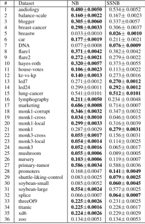
# Dataset NB SSNB 1 audiology 0.480±0.0050 0.534±0.0052 2 balance-scale 0.160±0.0022 0.167±0.0023 3 blogger 0.305±0.0060 0.337±0.0057 4 breast-cancer 0.298±0.0033 0.306±0.0037 5 breastw 0.033±0.0010 0.026±0.0010 6 car 0.177±0.0019 0.211±0.0021 7 DNA 0.077±0.0008 0.076±0.0009 8 flare1 0.371±0.0042 0.382±0.0042 9 flare2 0.272±0.0021 0.279±0.0022 10 hayes-roth 0.320±0.0057 0.373±0.0055 11 house-votes 0.106±0.0023 0.113±0.0022 12 kr-vs-kp 0.140±0.0013 0.273±0.0016 13 led7 0.271±0.0012 0.270±0.0012 14 led24 0.299±0.0011 0.292±0.0012 15 lung-cancer 0.541±0.0101 0.512±0.0101 16 lymphography 0.211±0.0050 0.234±0.0048 17 marketing 0.686±0.0008 0.714±0.0007 18 monk1-corrupt 0.346±0.0032 0.347±0.0032 19 monk1-cross 0.034±0.0010 0.046±0.0015 20 monk1-local 0.299±0.0033 0.316±0.0039 21 monk1 0.287±0.0029 0.279±0.0031 22 monk3-cross 0.055±0.0017 0.156±0.0031 23 monk3-local 0.054±0.0014 0.114±0.0025 24 monk3 0.052±0.0016 0.065±0.0017 25 mushroom 0.055±0.0006 0.089±0.0005 26 nursery 0.103±0.0006 0.119±0.0007 27 primary-tumor 0.586±0.0034 0.588±0.0036 28 promoters 0.168±0.0047 0.141±0.0049 29 shuttle-l&ing-control 0.083±0.0025 0.079±0.0025 30 soybean-small 0.085±0.0052 0.060±0.0045 31 soybean-large 0.554±0.0024 0.577±0.0025 32 splice 0.066±0.0007 0.064±0.0007 33 threeOf9 0.225±0.0026 0.231±0.0025 34 titanic 0.225±0.0016 0.228±0.0017 35 xd6 0.224±0.0026 0.229±0.0029 36 zoo 0.134±0.0051 0.134±0.0053
TABLE II. GLOBAL SCORE FORAULCFOR THENBANDSSNBOVER 20CONTINUOUS DATASETS FROMUCIREPOSITORY. THE RESULTS FOR
EACHAULCCLASSIFIER ARE PRESENTED IN THE FORM OF THE MEAN AND STANDARD ERROR OVER TEST DATA FOR100REALISATIONS OF EACH
DATASET.THE BOLDFACE FONT INDICATES THAT THE GLOBAL SCORE FOR ONE OF THE CLASSIFIERS IS BETTER THAN THE OTHER CLASSIFIER.
# Dataset NB SSNB 1 banknote 0.156±0.0021 0.244±0.0020 2 Blood-transfusion 0.252±0.0025 0.290±0.0035 3 breast-cancerw-continuous 0.040±0.0013 0.040±0.0014 4 Climate-Mode-Simulation-Crashes 0.067±0.0017 0.070±0.0017 5 glass 0.483±0.0049 0.554±0.0041 6 haberman 0.259±0.0040 0.279±0.0052 7 ionosphere 0.180±0.0044 0.237±0.0042 8 iris 0.063±0.0032 0.061±0.0031 9 letter 0.370±0.0006 0.508±0.0006 10 liver-disorder 0.442±0.0040 0.490±0.0043 11 magic04 0.274±0.0006 0.334±0.0006 12 musk1 0.283±0.0041 0.395±0.0035 13 new-thyroid 0.044±0.0022 0.034±0.0022 14 pendigits 0.155±0.0006 0.180±0.0008 15 sleep 0.341±0.0003 0.438±0.0004 16 vehicle 0.539±0.0027 0.600±0.0022 17 vowel 0.396±0.0031 0.488±0.0026 18 waveform-noise 0.202±0.0011 0.226±0.0010 19 waveform 0.232±0.0010 0.265±0.0011 20 wine 0.063±0.0023 0.041±0.0024 −80 −6 −4 −2 0 2 4 6 0.05 0.1 0.15 0.2 0.25 0.3 0.35 0.4 Class1: µ =−1: σ =1 Class2: µ =+1: σ =1
Fig. 1. Two class classification problem for the synthetic dataset
This experiment consisted of 10,000 trials of random partitioning of the datasets (67584 patterns) into training and test sets, that 2048 patterns were used for training and 65536 patterns were held-out as a test set used to evaluate the classification error rate performance during the experiments. The experimental design exactly same as section III-A1. Figure 2 shows the error rate learning curve for both the semi-supervised Gaussian classifier and the Gaussian classifier. It is clearly seen that the semi-supervised Gaussian classifier performs better than the Gaussian classifier, especially when very few labeled data were used for training, and rapidly converges in the number of labelled samples.
101 102 103 0.16 0.18 0.2 0.22 0.24 0.26 0.28 0.3 0.32
Labeled set size
error rate
NB SSNB
Fig. 2. The learning curve for two class classification problem in Gaussian distribution for synthetic dataset
C. Synthetic benchmark dataset
1) Generating synthetic dataset and experimental design:
The results from the previous section III-B indicate that the violation of the independence assumption of NB mode, might be a reason for the lack of increased performance for the SSNB. It is possible that the SSNB is sensitive to the correctness of the model’s assumptions. To investigate this further, we generate simulated data from the UCI sets that will satisfy the independence assumption. To do this, we first fit a NB model to each data set, then use the model estimates of the attribute distributions to generate simulated data with independent features. The synthetic datasets are similar in character to the original datasets but the model’s assumption of the independence of attributes is valid.
TABLE III. GLOBAL SCORE FORAULCFOR THENBANDSSNB OVER36SYNTHETIC DATASETS FROMUCI. THE RESULTS FOR EACH AULCCLASSIFIER ARE PRESENTED IN THE FORM OF THE MEAN AND STANDARD ERROR OVER TEST DATA FOR100REALISATIONS OF EACH DATASET.THE BOLDFACE FONT INDICATES THAT THE GLOBAL SCORE FOR
ONE OF THE CLASSIFIERS IS BETTER THAN THE OTHER CLASSIFIER.
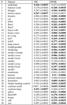
# Dataset NB SSNB 1 audiology 0.436±0.0055 0.437±0.0049 2 balance-scale 0.270±0.0026 0.268±0.0028 3 blogger 0.287±0.0062 0.284±0.0058 4 breast-cancer 0.267±0.0037 0.269±0.0037 5 breastw 0.004±0.0002 0.000±0.0000 6 car 0.247±0.0016 0.244±0.0017 7 DNA 0.033±0.0005 0.022±0.0005 8 flare1 0.298±0.0040 0.283±0.0039 9 flare2 0.201±0.0020 0.198±0.0020 10 hayes-roth 0.329±0.0054 0.314±0.0051 11 house-votes 0.001±0.0001 0.000±0.0000 12 kr-vs-kp 0.175±0.0013 0.168±0.0013 13 led7 0.271±0.0015 0.269±0.0015 14 led24 0.288±0.0012 0.277±0.0012 15 lung-cancer 0.187±0.0085 0.167±0.0090 16 lymphography 0.104±0.0032 0.066±0.0030 17 marketing 0.589±0.0007 0.586±0.0007 18 monk1-corrupt 0.287±0.0029 0.280±0.0031 19 monk1-cross 0.107±0.0021 0.086±0.0021 20 monk1-local 0.318±0.0031 0.310±0.0035 21 monk1 0.320±0.0030 0.320±0.0031 22 monk3-cross 0.090±0.0022 0.076±0.0023 23 monk3-local 0.122±0.0021 0.107±0.0020 24 monk3 0.116±0.0022 0.106±0.0024 25 mushroom 0.001±0.0001 0.001±0.0001 26 nursery 0.156±0.0006 0.15±0.0006 27 primary-tumor 0.560±0.0037 0.560±0.0038 28 promoters 0.063±0.0024 0.009±0.0015 29 shuttle-landing-control 0.101±0.0028 0.093±0.0029 30 soybean-small 0.067±0.0046 0.049±0.0045 31 soybean-large 0.451±0.0027 0.460±0.0027 32 splice 0.048±0.0005 0.032±0.0006 33 threeOf9 0.280±0.0032 0.270±0.0033 34 titanic 0.227±0.0015 0.226±0.0015 35 xd6 0.229±0.0029 0.219±0.0029 36 zoo 0.087±0.0042 0.081±0.0044
2) Result for synthetic benchmark datasets: Table III shows that the SSNB performs well compared to the NB for the 30 synthetic benchmark datasets. The SSNB also was best on 19 of the continuous synthetic datasets, shown in Table IV,thus the SSNB better than the NB in the current experiment.There is a statistical significant difference between the average rank of the SSNB and NB global scores for AULC according to the Wilcoxon signed rank test at the 95% level of confidence over multiple synthetic benchmark datasets. This suggest that SSNB is sensitive to conformance to its assumption of the independence between attributes.
D. Exploratory Data Analysis
The results for UCI benchmark datasets experiments
suggest that a few datasets are always likely
to have better performance for SSNB, such as
(breastw, DNA, led7, led24, lung-cancer,
promoters, shuttle-landing-control, splice,
soybean-small) in discrete and (iris, new-thyroid,
wine) in continuous benchmark datasets. The details of this performance can be seen by examing the learning curve. We can show learning curve only for a few datasets due to space limitation. Figure 3 shows the learning curve for one of the discrete datasets splice and new-thyroid which is the continuous datasets.
Interestingly, most of the benchmark datasets show improved classification performance for the SSNB in the synthetic
TABLE IV. GLOBAL SCORE FORAULCFOR THENBANDSSNB OVER20SYNTHETIC DATASETS FROMUCI. THE RESULTS FOR EACH AULCCLASSIFIER ARE PRESENTED IN THE FORM OF THE MEAN AND STANDARD ERROR OVER TEST DATA FOR100REALISATIONS OF EACH DATASET. THE BOLDFACE FONT INDICATES THAT THE GLOBAL SCORE FOR
ONE OF THE CLASSIFIERS IS BETTER THAN THE OTHER CLASSIFIER.
# Dataset NB SSNB 1 banknote 0.201±0.0016 0.197±0.0018 2 Blood-transfusion 0.093±0.0017 0.087±0.0018 3 breast-cancerw-continuous 0.002±0.0002 0.000±0.0001 4 Climate-Mode-Simulation-Crashes 0.008±0.0006 0.004±0.0004 5 glass 0.126±0.0033 0.105±0.0033 6 haberman 0.184±0.0041 0.175±0.0042 7 ionosphere 0.008±0.0005 0.002±0.0003 8 iris 0.004±0.0008 0.001±0.0005 9 letter 0.236±0.0005 0.223±0.0006 10 liver-disorder 0.217±0.0033 0.198±0.0035 11 magic04 0.006±0.0001 0.006±0.0001 12 musk1 0.014±0.0008 0.007±0.0006 13 new-thyroid 0.006±0.0006 0.001±0.0005 14 pendigits 0.065±0.0003 0.059±0.0003 15 sleep 0.128±0.0002 0.127±0.0002 16 vehicle 0.247±0.0020 0.241±0.0020 17 vowel 0.108±0.0017 0.071±0.0017 18 waveform-noise 0.020±0.0003 0.017±0.0003 19 waveform 0.052±0.0005 0.049±0.0005 20 wine 0.010±0.0008 0.003±0.0006 100 102 0 0.2 0.4 0.6 0.8 splice data error rate NB SSNB 100 102 0 0.2 0.4 0.6 0.8
splice synthetic data
error rate 102 0 0.1 0.2 0.3 0.4
new thyroid data
Labeled set size
error rate 102 0 0.1 0.2 0.3 0.4
new thyroid synthetic data
Labeled set size
error rate
Fig. 3. The average learning curve for NB and SSNB of the UCI and synthetic (splice, newthyroid) datasets
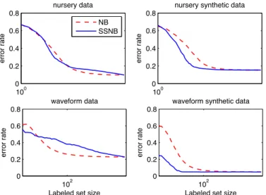
datasets. Figure 4 shows the learning curve for nursery and waveform datasets which are discrete and continuous respectively. However, learning curve for (audiology,
breast-cancer,monk1,mushroom,primary-tumor,
soybean-large) in discrete datasets and (magic04) in continuous datasets show that SSNB does not help in all experiments, as we can see learning curve for one of them in figure 5.
The learning curve results across all experiments shows that if the model assumption is correct the unlableled data might help to improving performance, especially when a few lableled data used as a training set, but if the model assumption is violated, the classififcation performance could degrade as adding more unlableled to the training set.
100 0 0.2 0.4 0.6 0.8 nursery data error rate NB SSNB 100 0 0.2 0.4 0.6 0.8
nursery synthetic data
error rate 102 0 0.2 0.4 0.6 0.8 waveform data
Labeled set size
error rate 102 0 0.2 0.4 0.6 0.8
waveform synthetic data
Labeled set size
error rate
Fig. 4. The average learning curve for the NB and SSNB of the UCI and synthetic (nursery, waveform) datasets
100 102
0 0.5 1
audiology data
Labeled set size
error rate NB SSNB 100 102 0 0.5 1
audiology synthetic data
Labeled set size
error rate
Fig. 5. The average learning curve for the NB and SSNB of the UCI and synthetic audiology datasets
IV. CONCLUSION
The contribution of this paper is an empirical evaluation of NB and SSNB on binary and multi-class classification problems with continuous and discrete attributes. We wish to address the question of whether using unlabelled data will improve classification accuracy. This will clearly be dictated by our choice of classifier and semi-supervised learning scheme. We evaluate a na¨ıve Bayes classifier used in conjunction with an Expectation-Maximization algorithm that iteratively uses NB to predict the unlabelled instances. We found that using the unlabelled data made the classifier significantly less accurate. To understand why this may be so, we assessed the performance of NB and SSNB on synthetic data for which the NB assumption of independent attributes is true. We found that SSNB was significantly more accurate on these data. We conclude that if a classifier is not suitable for a data set, then using unlabelled data in a self training scheme is likely to make it worse. This implies that effort should be applied in finding a classifier suitable for a problem before using unlabelled data to self train.
REFERENCES
[1] X. Zhu, “Semi-supervised learning literature survey,” 2006.
[2] K. Nigam, A. McCallum, and T. Mitchell, “Semi-supervised text classification using EM,”Semi-Supervised Learning, pp. 33–56, 2006.
[3] F. G. Cozman and I. Cohen, “Unlabeled data can degrade classification performance of generative classifiers,” in Proceedings of the Fifteenth International Florida Artificial Intelligence
Research Society Conference, May 14-16, 2002, Pensacola
Beach, Florida, USA, 2002, pp. 327–331. [Online]. Available: http://www.aaai.org/Library/FLAIRS/2002/flairs02-065.php
[4] Y. Guo, X. Niu, and H. Zhang, “An extensive empirical study on semi-supervised learning,” in Data Mining (ICDM), 2010 IEEE 10th International Conference on. IEEE, 2010, pp. 186–195.
[5] R. O. Duda and P. E. Hart, “Pattern Recognition and Scene Analysis,” 1973.
[6] A. P. Dempster, N. M. Laird, and D. B. Rubin, “Maximum likelihood from incomplete data via the EM algorithm,” Journal of the Royal Statistical Society. Series B (Methodological), vol. 39, no. 1, pp. 1– 38, 1977.
[7] C.-H. Lee, F. Gutierrez, and D. Dou, “Calculating feature weights in naive Bayes with Kullback-Leibler measure,” inData Mining (ICDM), 2011 IEEE 11th International Conference on. IEEE, 2011, pp. 1146– 1151.
[8] L. Jiang, Z. Cai, H. Zhang, and D. Wang, “Not so greedy: Randomly selected naive Bayes,”Expert Systems with Applications, vol. 39, no. 12, pp. 11 022–11 028, 2012.
[9] P. Langley, W. Iba, and K. Thompson, “An Analysis of Bayesian Classifiers.” in Proceedings of the 10th National Conference on Artificial Intelligence. San Jose, CA, July 12-16, 1992., 1992, pp. 223–228. [Online]. Available: http://www.aaai.org/Library/AAAI/1992/aaai92-035.php
[10] D. Klein, “Lagrange multipliers without permanent scarring,”University of California at Berkeley, Computer Science Division, 2001.
[11] J. Wu and Z. Cai, “A naive Bayes probability estimation model based on self-adaptive differential evolution.” Journal of Intelligent Information Systems, vol. 42, no. 3, pp. 671–694, 2014. [Online]. Available: http://dx.doi.org/10.1007/s10844-013-0279-y
[12] K. Nigam, A. K. McCallum, S. Thrun, and T. Mitchell, “Text classi-fication from labeled and unlabeled documents using EM,” Machine learning, vol. 39, no. 2-3, pp. 103–134, 2000.
[13] K. Bache and M. Lichman, “UCI Machine Learning Repository,” 2013. [Online]. Available: http://archive.ics.uci.edu/ml
[14] I. Guyon, G. Cawley, G. Dror, and V. Lemaire, “Results of the active learning challenge,”Active Learning Challenge Challenges in Machine Learning, Volume 6, p. 21.
[15] J. Demˇsar, “Statistical comparisons of classifiers over multiple data sets,” The Journal of Machine Learning Research, vol. 7, pp. 1–30, 2006.