University of Padova
Department of Information Engineering
Master Thesis inICT for Internet and Multimedia
Distributed Deep Reinforcement
Learning for Drone Swarm Control
Supervisor Master Candidate
Prof. Alberto Testolin Federico Venturini
University of Padova
Department of General Psychology
Co-supervisor
Prof. Andrea Zanella
Abstract
Reinforcement Learning is a promising Machine Learning field that has started to be widely used in many scenarios, from robotics to chemistry. Inspired by the way humans learn, it consists of an iterative approach in which an agent, by interacting with and receiving feed-back from its environment, attempts to learn an optimal action selection policy.
In this project we applied Deep-Q Reinforcement Learning, a technique that combines the power of Deep Learning, in particular of Convolutional Neural Networks (CNNs), with the Q-Learning approach, to manage a swarm scenario in a bi-dimensional environment. Given a square map with some targets, the goal is to make the drones able to learn to cooperate be-tween them, trying to track and follow the most valuable targets. We compared a distributed and a centralized approach and verified how the first can outperform the latter in a real-world scenario with limited training.
Contents
Abstract v List of figures ix 1 Introduction 1 2 Reinforcement Learning 5 2.0.1 Elements of Reinforcement . . . 72.1 Finite Markov Decision Processes . . . 8
2.1.1 The agent-Environment Interface . . . 8
2.1.2 Goals and rewards . . . 9
2.1.3 Returns and episodes . . . 9
2.1.4 Policies and value functions . . . 10
2.1.5 Optimal policies and optimal value functions . . . 11
2.2 Dynamic programming . . . 13
2.3 Monte Carlo methods . . . 14
2.3.1 Monte Carlo estimation of action values . . . 14
2.3.2 Monte Carlo control . . . 15
2.3.3 Monte Carlo control without ES . . . 16
2.4 Temporal Difference Reinforcement Learning . . . 17
2.4.1 TD prediction . . . 18
2.4.2 Advantages of TD prediction methods . . . 19
2.4.3 Optimality of TD(0) . . . 19
2.4.4 Sarsa: on-policy TD control . . . 20
2.4.5 Q-learning: Off-policy TD control . . . 21
2.4.6 Expected Sarsa . . . 21
2.4.7 Maximization bias and double learning . . . 22
2.4.8 Exploration vs Exploitation . . . 23
2.5 Neural Networks . . . 26
2.5.1 Fully Connected neural network . . . 26
2.5.2 Convolutional Neural Networks . . . 29
3 System model 35
3.1 Environment . . . 35
3.1.1 Single drone scenario . . . 37
3.1.2 Swarm scenario . . . 38
3.2 Techniques . . . 40
3.2.1 Neural networks . . . 40
3.2.2 Pre-training . . . 43
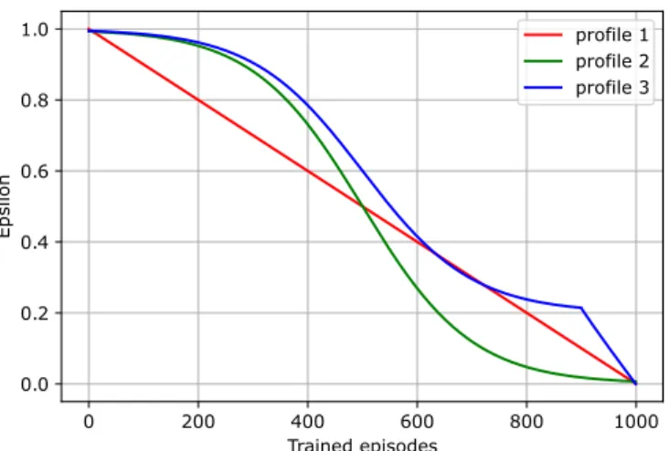
3.2.3 Exploration policies . . . 43
3.2.4 Learning - how to train . . . 43
3.2.5 Hyper-parameters Optimization Search . . . 45
4 Results - single drone scenario 49 4.1 One drone, one target . . . 49
4.1.1 Reinforcement Learning optimization . . . 49
4.1.2 Peak invariance . . . 53
4.2 One drone, two targets . . . 54
5 Results -swarm scenario 59 5.1 Distributed version . . . 59
5.1.1 Hyper-parameters optimization search . . . 59
5.1.2 How to learn - memory replay settings . . . 60
5.1.3 2 targets vs 3 targets models . . . 61
5.1.4 Inference - more targets . . . 63
5.1.5 Inference - 1 drone . . . 63
5.2 Centralized version . . . 64
5.2.1 Computation of the centralized reward . . . 64
5.2.2 Comparison with distributed . . . 65
6 Conclusion 67
References 70
Listing of figures
2.1 Reinforcement Learning framework . . . 8
2.2 Fully connected neural network example . . . 26
2.3 ReLU . . . 27
2.4 Learnig rate definition. . . 28
2.5 CNN example . . . 29
2.6 2D Convolution . . . 30
2.7 Pooling example. . . 31
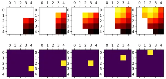
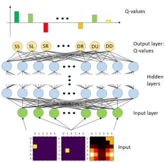
3.1 Input of the single drone neural network. . . 36
3.2 Environment’s dynamics. . . 36
3.3 Single drone neural network case . . . 41
3.4 Distributed neural network case . . . 41
3.5 Centralized neural network case (2 drones) . . . 42
3.6 Exploration policies. . . 44
3.7 Personalized Hyper-parameters search. . . 48
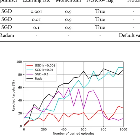
4.1 Results learning rate. . . 50
4.2 Gamma performances. . . 51
4.3 Bigger map, more training. . . 52
4.4 Epsilon performances. . . 53
4.5 Peak invariance. . . 53
4.6 Inference - number of targets. . . 54
4.7 Comparison among 3 models . . . 54
4.8 Successful test episode. . . 55
4.9 Successful test episode . . . 55
4.10 Comparison with heuristic approach - performance . . . 56
4.11 Comparison with heuristic - inference time . . . 56
5.1 Performances of all hyper-parameters combinations. . . 60
5.2 Result memory-replay settings. . . 60
5.3 2 targets vs 3 targets . . . 61
5.4 Successful distributed multi drone example . . . 62
5.5 Successful distributed multi drone example . . . 62
5.6 Inference - number of targets . . . 63
5.8 Reward type. . . 64 5.9 Centralized vs Distributed . . . 65
1
Introduction
In the last decade, thanks to the continuing growth of computing power, Machine Learn-ing became a must in many fields. It is very useful for the analysis of a big amount of data and the creation of models able to outperform any complex human model designed. In the context of complex scenarios, the design of engineered models is very time consuming and difficult. Instead of tuning the features of the models, in Machine Learning these are ex-tracted from data. We can talk in this way of a model-free approach. Among the various techniques used in Machine Learning, Neural Networks are nowadays the most common. In particular Deep Neural Networks (DNNs) are state-of-the-art techniques: using the par-allel computing power of Graphics Processing Units (GPUs), they are able to construct very complex models that manage and benefit from large amounts of data. They are used in a va-riety of tasks, including computer vision [1], speech recognition [2][3], machine translation [4], social network filtering etc.
In the last years Neural Networks have been combined with Reinforcement Learning (RL), and in particular with Q-Learning [5]. For this reason, now we talk about Deep Reinforce-ment Learning applications and Deep-Q-Networks (DQN).
Reinforcement Learning is a sub-field of Machine Learning where an agent that interacts with an environment learns an optimal action selection policy by receiving feedback from it. RL algorithms learn in an iterative way: at each iteration the learner observes its state, it chooses an action that leads to a subsequent environment’s state. Then, the learner receives
a reward or a penalty and updates its value function, which represents the objective to maxi-mize. Exploring the environment and collecting this informations the agents learns how to maximize the long-term reward.
Recently Artificial Intelligence reached incredible results, with the use of RL. It has been hugely successful in classic table games, like chess or Go. These games imply solving a search problem at each move, and RL amazingly boosts the efficiency of the search. AlphaGo be-came the first program to defeat a human world champion in the game of Go [6].
Classic video games are other good benchmarks because they are executable environments with large state spaces. With the use of a DQN, an agent was trained and tested on the chal-lenging domain of classic Atari 2600 games [7]. It has been demonstrated that the DQN agent, was able to surpass the performance of all previous algorithms and achieve a level com-parable to that of a professional human games tester across a set of 49 games receiving only the pixels and the game score as inputs. RL has also been applied to solve a Rubik’s cube with a humanoid robot hand [8].
However, RL is also applicable in many real world scenarios: from the design of a traffic light controller to solve the congestion problem [9], to the optimization of chemical reac-tions [10] or personalized recommendations systems [11]. The list of other possible applica-tions in which RL can be applied is vast. One of them is the coordination of a multi-agent system. These situations arise naturally in a variety of domains, such as: robotics, telecom-munications, drones, economics, distributed control, auctions, traffic light control, etc. In such systems it is important that agents are capable of discovering good solutions to the prob-lem at hand either by coordinating with other learners or by competing with them.
The drone scenario is the one chosen for this project. Drones can be used for search and rescue operations [12], for aerial filming, for security reasons, for maintenance, for environ-mental monitoring [13], delivery services [13] and many other situations. In this work we ap-plied Deep-Q-Learning, using Conv. Neur. Networks (CNNs), to train a swarm of drones to cooperate in a grid world. The objective is to explore a map and track any number of targets, which might move around the map, have different values over time and space, or ap-pear or disapap-pear suddenly. In this thesis, we limited ourselves to a static case, in which the problem simplifies to the assignment of a target to each drone. We compared a distributed approach and a centralized one. A similar work on a multi-agent cooperation was developed by Egorov [14], where a pursuit-evasion game has been simulated, with two pursuers that
try to catch two evaders.
The structure of the rest of this thesis is as follows:
in Chapter II we present an introduction to RL, presenting the Markov Decision Processes (MDP) model and the Temporal Difference (TD) learning solution. In particular, the Deep-Learning approach is presented , with the application of Neural Networks on the Q-Learning.
In Chapter III we describe our drone swarm scenario and how we implemented Deep-Q-Learning. Some Reinforcement Learning strategies are also described and the way we con-ducted Optimization Search on some hyper-parameters is presented.
In Chapter IV there are the results of a single drone scenario: how it behaves in a single target situation and in a multi targets one, how it scales with the world size and how much some parameters can affect the final performance.
In Section V we analyze the results of a swarm situation, with the comparison between a dis-tributed and centralized approach, the study of a generalization on more complex situations and the benefits of the learning strategies and the Optimization Search described in Section III.
In Section VI we briefly analyze the results obtained, we try to propose some ways to increase the performances and we present the numerous theoretical extensions that this project could have.
2
Reinforcement Learning
In this chapter, we present an introduction to the Reinforcement Learning concepts that we will use in our work [15]. Then, the Deep-Q-Learning approach is described with a general overview on neural networks, and on Convolutional Neural Networks in particular.
What is Reinforcement Learning
Reinforcement Learning [15, Sec.I] is a sub field of Machine Learning. Machine Learn-ing can be divided into 3 main areas:
• Supervised Learning • Unsupervised Learning • Reinforcement Learning
Supervised learning is learning from a training set of labeled examples provided by a knowl-edgeable external supervisor. Each example is a description of a situation together with a specification (the label) of the correct output the system should take in that situation. We can, in general, classify the main tasks of Supervised Learning in classification tasks and re-gression tasks.
collections of unlabeled data. Clustering and dimensionality reduction are the main appli-cations of this kind of learning.
Although one might be tempted to think of Reinforcement Learning as a kind of unsuper-vised learning, it is trying to maximize a reward signal instead of trying to find hidden struc-tures in the data. We can say that RL means ”how to map situations to actions”. The learner is not told which actions to take, but instead must discover which actions yield the most re-ward by trying them. In the most interesting and challenging cases, actions may affect not only the immediate reward but also the next situation and all subsequent rewards. Since the learner receives a scalar value as consequent feedback of its action, we could classify RL as a supervised approach. But in the latter case the feedback received, the label, is sufficient to know the correct output of the model, in the RL case it is only a scalar that helps to find it. The two features, trial-and-error search and delayed reward, are the two most important distinguishing features of Reinforcement Learning.
Main features of RL are:
• Its goal is to design algorithms (agents) that learn to make actions in order to maximize the sum of the cumulated following reward
• The agent’s initial knowledge about the environment is limited
• The agent learns by trial and error: after selecting an action, the agent observes the effects of the action on the environment, and receives a feedback signal (reward) What makes it different from other areas in Machine Learning:
• There is no supervisor, only a reward signal • Feedback is delayed, not immediate
• Time matters (data is received sequentially)
2.0.1 Elements of Reinforcement
• Policy: it defines the learning agent’s way of behaving at a given time. It is a mapping from perceived states of the environment to actions to be taken when in those states. • Reward signal: it defines the goal of a RL problem. At each time step, the
environ-ment sends a scalar called reward to the RL agent. The agent’s objective is to maximize the total reward it receives over the long run.
• Value function: while a reward indicates what is good in an immediate sense, a value function specifies what is good in the long run. The value of a state is the total amount of reward an agent can expect to accumulate in the future, starting from that state. A state might yield a low immediate reward but still have an high value because it is regularly followed by other states that yield high rewards. We prefer actions that lead to states of highest value, not highest reward.
• Model environment: it’s something that mimics the behavior of the environment, or more generally, that allows inferences to be made about how the environment will behave. Given a state and action, the model might predict the resultant next state and next reward.
2.1 Finite Markov Decision Processes 2.1.1 The agent-Environment Interface
Figure 2.1:Reinforcement Learning framework
The agent and environment interact at each of a sequence of discrete time steps, t=0,1,2,3,... At each time step t, the agent receives some representation of the environment’s state,st ∈S, and on that basis selects an action,at∈A(s). One time step later, in part as a consequence of its action, the agent receives a numerical reward,rt+1 ∈R, and finds itself in a new state,
st+1[15, Sec. III]. The MDP and agent together thereby give rise to a sequence or trajectory
that begins like this:
s0, a0, r1, s1, a1, r2, s2, a2, r3, ...
In a finite MDP, the sets of states, actions and rewards (S,A,R) all have a finite number of elements. In this case, the random variablesStandRthave well defined discrete probability distributions dependent only on the preceding state and action:
p(s′, r|s, a) = P r[St=s ′ , Rt=r|St−1 =s, At−1 =a]∀s ′ , s∈S, r∈R, a∈A(s) (2.1) The function p defines the dynamics of the MDP and is an ordinary deterministic function with 4 arguments: ∑ s′∈S ∑ r∈R p(s′, r|s, a) = 1∀s∈S, a∈A(s) (2.2)
In a MDP, the state-transition and reward probability distributions completely characterize the environment’s dynamics. The probability of each possible value forStandRtdepends
only on the immediately preceding state and action,St−1andAt−1, and, given them, not at
all on earlier states and actions. This is a restriction on the state, not on the decision process. The state must include information about all aspects of the past agent-environment interac-tion that make a difference for the future. If it does, then we have the Markov property.
p(s′|s, a) = P r[St=s ′ |St−1 =s, At−1 =a] = ∑ r∈R p(s′, r|s, a) (2.3) r(s, a) =E[Rt|St−1 =s, At−1 =a] = ∑ r∈R r∑ s′∈S p(s′, r|s, a) (2.4) r(s, a, s′) = E[Rt|St−1 =s, At−1 =a, St =s ′ ] =∑ r∈R rp(s ′ , r|s, a) p(s′|s, a) (2.5)
2.1.2 Goals and rewards
If we want to make a robot learn how to escape from a maze, the reward is often -1 for every time step that passes prior to escape; this encourages the agent to escape as quickly as possible. One might also want to give the robot negative rewards when it bumps into things or when somebody yells at it. Instead, for an agent that has to learn to play chess, we can use +1 for winning, -1 for loosing and 0 reward for all non-terminal positions.
It is thus critical that the rewards we set up truly indicate what we have in mind. The reward is our way of communicating to the robot what we want to achieve, not how we want it achieved (a chess player should be rewarded only for actually winning, not for achieving sub-goals such as taking it’s opponent’s pieces or gaining control of the center of the board. If achieving these sorts of sub-goals were rewarded, then agent might find a way to achieve them without achieving the goal).
2.1.3 Returns and episodes
In general we seek to maximize the expected return, where the return, denotedGt, is defined as some specific function of the reward sequence. In the simplest case, the return is the sum of the expected reward:
Gt =rt+1+rt+2+...+rT (2.6) where T is a random variable which represents the final step. This approach makes sense in applications in which there is a natural notion of the final step. Each episode ends in a
spe-cial state called ”terminal state”, followed by a reset to a standard starting state or to a sample from a standard distribution of starting states. The next episode begins independently of how the previous one ended. Thus the episodes can all be considered to end in the same terminal state, with different rewards for the different outcomes. These are called episodic tasks.
On the other hand, in many cases the agent-environment interaction does not break natu-rally into identifiable episodes, but goes on without limits. This would be a natural way to formulate an on-going process-control task and manage in this way continuing tasks. Com-putingGtis problematic for continuing tasks because the final step would be T=∞, and the return could easily infinite. For this reason a discounting factor is used:
Gt=Rt+1+γRt+2+γ2Rt+3+...= (2.7) = ∞ ∑ k=0 γkRt+k+1 0≤γ ≤ 1 :discount rate (2.8)
Ifγ <1, the infinite sum has a finite value as long as the reward sequence{Rk}is bounded. Gt=Rt+1+γRt+2+γ2Rt+3+...=Rt+1+γ(Rt+2+γRt+3+...) = Rt+1+γGt+1 (2.9)
This works for all time steps t<T, even if termination occurs at t+1, if we defineGT = 0. Al-though the return is a sum of an infinite number of terms, it still converges to a finite value if the reward is non-zero and bounded, ifγ <1. For example if the reward is +1,
Gt= ∞ ∑ k=0 γk= 1 1−γ (2.10)
2.1.4 Policies and value functions
A policy is a mapping from states to probabilities of selecting each possible action:
π : s → p(a|s)∀a ∈ A. If the agent is following policyπat time t, thenπ(a|s)is the
probability thatAt=aifSt=s. The value function of a state s under a policyπ,vπ(s), is the expected return when starting in s and followingπ(the value of the terminal state, if any,
is always 0): vπ(s) =Eπ = [Gt|St=s] =Eπ[ ∞ ∑ k=0 γkRt+k+1|St=s],∀s∈S (2.11)
Equation is defined as state-value function for policyπ. We define the value of taking action a in state s under a policyπ,qπ(s, a), as the expected return starting from s, taking the action a and followingπ: qπ(s, a) =Eπ[Gt|St =s, At=a] =Eπ[ ∞ ∑ k=0 γkRt+k+1|St =s, At=a] (2.12)
vπandqπcan be estimated from experience. If an agent follows policyπand maintains an average, for each state encountered, of the actual returns that have followed that, then the av-erage will converge to the state’s valuevπ(s)as the number of times that state is encountered approaches infinity. If separate averages are kept for each action taken in each state, then the averages will similarly converge to the action valuesqπ(s, a). These methods are called Monte Carlo methods because they involve averaging over many random samples of actual returns. vπ(s) = Eπ[Gt|St=s] =Eπ[Rt+1+γGt+1|St =s] = (2.13) =∑ a π(a|s)∑ s′ ∑ r p(s′, r|s, a)[r+γEπ[Gt+1|St+1 =s′] (2.14) =∑ a π(a|s)∑ s′,r p(s′, r|s, a)[r+γvπ(s′)]∀s ∈S (2.15) Equation 2.14 is called ”Bellman equation forvπ”, and it expresses a relationship between the value of a state and the values of its successor values; the value of the state must be equal to the (discounted) value of the expected next state, plus the reward expected along the way. The value functionvπis the unique solution to its Bellman equation.
2.1.5 Optimal policies and optimal value functions
A policyπis defined to be better than or equal to a policyπ′if its expected return is greater than or equal to that ofπ′for all states:
There is always at least one policy that is better than or equal to all other policies: it’s the optimal policy. Although there may be more than one, we denote all the optimal policies by π∗. They share all the same-value function, called optimal state-value function:
v∗(s) = max
π vπ(s)∀s∈S (2.17)
Optimal policies also share the same optimal-action value function:
q∗(s, a) = max
π qπ(s, a)∀s ∈S, a∈A(s) (2.18)
→q∗(s, a) = E[Rt+1+γV∗(St+1)|St=s, At =a] (2.19) Becausev∗ is the value function for a policy, it must satisfy the self-consistency condition given by the Bellman equation, for state values. Because it’s the optimal value function, however,v∗’s consistency condition can be written in a special form without reference to any specific policy. This is the Bellman equation forvπ, or the Bellman optimality equation, that intuitively expresses the fact that the value of a state under an optimal policy must be equal to the expected return for the best action from that state:
v∗(s) = max a∈A(s)qπ∗(s, a) = maxa Eπ∗[Gt|St=s, At =a] = (2.20) = max a Eπ∗[Rt+1+γGt+1|St=s, At=a] = (2.21) = max a E[Rt+1+γv∗(St+1)|St=s, At =a] (2.22) = max a ∑ s′,r p(s′, r|s, a)[r+γv∗(s′)] (2.23) q∗(s, a) =E[Rt+1+γmax a′ q∗(St+1, a ′)|S t =s, At=a] (2.24) =∑ s′,r p(s′, r|s, a)[r+γmax a′ q∗(s ′, a′)] (2.25)
For finite MDPs, the Bellman optimality equation forvπhas a unique solution independent of the policy. The Bellman optimality equation is actually a system of equations, one for each state. So if there are n states, then, there are n equations in n unknowns. If the dynamics of the environment are known, then in principle one can solve this system of equations forv∗ using any one of a variety of methods for solving system of equations of non-linear equations.
Withv∗, it’s easy to obtain an optimal policy. For each state s, there will be one or more actions at which the maximum is obtained in the Bellman optimality equation. Any policy that assigns non-zero probability only to these actions is an optimal policy.
2.2 Dynamic programming
Dynamic programming refers to a collection of algorithms that can be used to compute optimal policies given a perfect model of the environment as a Markon Decision Process (MDP)[15, Sec. IV]. Classical DP algorithms are of limited utility in RL both because of their assumption of a perfect model and because of their computational expense. Usually, other methods are used: methods that try to achieve the same results of DP but with less computation and without assumption of perfect environment’s model. With DP, the as-sumptions are based on finite MDP: it’s state, action and reward sets, (S,A,R) are finite. The dynamics are given by a set of probabilities
p(s’,r|s,a)∀s∈S, a∈A(s), r∈R and s∈S
Although DP ideas can be applied to problems with continuous state and action spaces, ex-act solutions are possible only in special cases. With continuous states and ex-actions, state and action spaces are quantized and then applied finite-state DP methods.
The existence and uniqueness ofvπare guaranteed as long as eitherγ <1or eventual termi-nation is guaranteed from all states under the policyπ.
If the environment’s dynamics are completely known, then vπ(s) = ∑ a π(a|s)∑ s′,r p(s′, r|s, a)[r+γvπ(s′)] (2.26)
is a system of |S| simultaneous equations in |S| unknowns.
If we consider a sequence of approximate value functionsv0, v1, v2, ...each mappingS+to
R,v0is chosen arbitrarily and each successive approximation is obtained by using Bellman
equation forvπas an update rule:
vk+1(s) =Eπ[Rt+1+γvk(St+1)|St=s] = (2.27) =∑ a π(a|s)∑ s′,r p(s′, r|s, a)[r+γvk(s′)]∀s∈S (2.28)
vk = vπ is a fixed point for this update rule because the Bellman equation forvπ assures us of equality in this case. The sequencevk can be shown in general to converge tovπ as k → ∞under the same conditions that guarantee the existence ofvπ. Fromvktovk+1,
iter-ative policy evaluation applies the same operation to each state s: it replaces the old values of the successor state s, and the expected immediate rewards, along all the one-step transitions possible under the policy being evaluated: expected update. Each iteration of iterative policy evaluation updates the value of every state once to produce the new approximate value func-tionvk+1. All the updates done in DP algorithms are called expected updates because they
are based on the expectation over all possible next states rather than on a sample next state. 2.3 Monte Carlo methods
In Monte Carlo methods we don’t assume complete knowledge of the environment. We need only experience: sample sequences of states, actions and rewards from actual or simu-lated interaction with an environment. No prior knowledge of the environment is required. Although a model is required, the model need only generate sample transitions, not the complete probability distributions of all possible transitions that is required for dynamic programming. Only on the completion of an episode the values estimates and policies are changed.
The value of a state is the simply average of the returns observed after visits to that state. As more returns are observed, the average should converge to the expected value. Each oc-currence in a state s is called ”a visit to s”. There exist 2 possible methods: theFirst Visit MC method(it estimatesvπ(s)as the average of the returns following first visit to s) and the
Every-visit MC method(it averages the returns following all visits to s) [15, Sec. V]. 2.3.1 Monte Carlo estimation of action values
If a model is not available, then it’s particularly useful to estimate action values rather than state values. With a model, state values alone are sufficient to determine a policy. Without a model, they are not. One must explicitly estimate the value of each action in order for the values to be useful in suggesting a policy. Our goal is always to estimateq∗. BothFirst-visit
MCandEvery-visit MCconverge quadratically to the true expected values as the number of visits to each state-action pair→ ∞. But many state-action pairs may never be visited. Ifπ is a deterministic policy, then following it one will observe returns only for one of the action
for each state. With no returns to average, the Monte Carlo estimates of the other actions will not improve with experience.
This is the general problem of maintaining exploration. For policy evaluation to work for action values, we must assure continual exploration. One way to do this is by specifying that the episodes start in a state-action pair, and that every pair has a non-zero probability of being selected as the start. This guarantees that all state-action pairs will be visited an infinite number of times in the limit of an infinite number of episodes. This requirement is called the assumption ofexploring starts(ES). But exploring starts cannot generalize all the case as the best option.
2.3.2 Monte Carlo control
Many episodes are experienced, with the approximate action-value function approaching the true function asymptotically. Let us assume that episodes are generated with exploring starts, and an infinite number of episodes. Under these assumptions, Monte Carlo methods will compute eachqπkexactly, for arbitraryπk. Policy improvement is done by making the policy
greedy with respect to the current value function. In this case we have an action-value func-tion, and therefore no model is needed to construct the greedy policy: for any action-value function q, the corresponding greedy policy is the one that, for eachs∈S, deterministically chooses an action with maximal action-value:
π(s) = argmax
a q(s, a) (2.29)
Policy improvement then can be done by constructing eachπk+1as the greedy policy with
respect toqπk.
qπk(s, πk+1(s)) =qπk(s, argmax
a qπk(s, a)) = (2.30) = max
a qπk(s, a)≥qπk(s, πk(s)≥vπk(s) (2.31) The theorem assures that eachπk+1is uniformly better thanπk, or just good asπk, in which case they are both optimal policies. This assures that the overall process converges to the optimal policy and optimal value function. But there are 2 unlikely assumptions:
1. episodes have exploring starts 2. Infinite number of episodes
1. One is to hold firm to the idea of approximatingqπk in each policy evaluation.
Mea-surement and assumptions are made to obtain bounds on the magnitude and error probability in the estimates, and then sufficient steps are taken during each policy evaluation to assure that these bounds are sufficiently small. We will have correct con-vergence up to some level of approximation, but it also requires far too many episodes to be useful.
2. We give up trying to complete policy evaluation before returning to policy improve-ment. On each evaluation step we move the value function towardqπk, but we don’t
expect to actually get close over many steps. 2.3.3 Monte Carlo control without ES
The only general way to ensure that all actions are selected infinitely often is for the agent to continue to select them. There are 2 possible approaches:
1. On-policy methods 2. Off-policy methods
On-policy methods attempt to evaluate or improve a policy different from that used to gen-erate the data. Monte Carlo with ES method is an example. The policy is generally soft, meaning thatπ(a|s)>0 ∀s∈S and all a∈A(s), but gradually shifted closer and closer to a deterministic optimal policy→ ϵ−greedy. All non greedy actions are given the minimal probability of selection, ϵ
|A(s)|, and the remaining to the greedy action:1−ϵ+
ϵ
|A(s)|.
ϵ-greedy policies are examples ofϵ-soft policies, defined as policies for whichπ(a|s)≥ |A(ϵs)|
for all states and actions, for someϵ>0. Amongϵ-soft policies,ϵ-greedy policies are in some sense those that are closest to greedy.
As in Monte Carlo ES, we useFirst-visit MCmethods to estimate the action-value function for the current policy. Without the assumption of ES, however, we cannot simply improve the policy by making it greedy with respect to the current value function, because that would prevent further exploration of non-greedy actions. General policy improvement does not re-quire that the policy be taken all the way to a greedy policy, only that it be moved toward a greedy policy. In our on-policy method we will move it only to anϵ-greedy policy. For any ϵ-soft policy,π, anyϵ-greedy policy with respect toqπis guaranteed to be better than or equal toπby the policy improvement theorem.
but for a near-optimal policy that still explores. A possible solution is to use 2 policies: one that is learned about and that becomes the optimal policy, and one that is more exploratory and is used to generate behavior. They are called respectively,target policyandbehavior pol-icy. In this case the learning is from data ”off” the target policy: for this reason it is called Off-policy learning. On-policy methods are generally simple. Off-policy methods require additional concepts and notation, and because the data is due to a different policy, they are often of greater variance and slower to converge. On the other hand, off-policy methods are more powerful and general: they include on-policy methods as the special case in which the target and behavior policies are the same. On policy methods estimate the value of a policy while using it for control. In off-policy methods there 2 functions are separated. The policy used to generate behavior, thebehavior policy, may in fact be unrelated to the policy that is evaluated and improved, thetarget policy. Possible advantage: the target policy may be deter-ministic (e.g. greedy), while the behavior policy can continue to sample all possible actions. Off policy Monte Carlo control methods follow the behavior policy while learning about and improving the target policy. The behavior policy must have a non-zero probability of selecting all actions that may be selected by the target policy. To explore all possibilities, we require that the behavior policy be soft (that it select all actions in all states with non-zero probabilities).
The target policyπ∗is the greedy policy with respect to Q, which is an estimate ofqπ. The be-havior policy b can be anything, but in order to assure convergence ofπto the optimal policy, an infinite number of returns must be obtained for each pair of state and action. This can be assured by choosing b to beϵ-soft. The policyπconverges to optimal at all encountered even though actions are selected according to a different soft policy b, which may change between or even within episodes. Possible problem: this methods learns only from the tails of episodes, when all of the remaining actions in the episode are greedy. If non-greedy ac-tions are common, then learning will be slow, particularly for states appearing in the early portions of long episodes.
2.4 Temporal Difference Reinforcement Learning
Temporal Difference (TD) learning [15, Sec. VI] is a combination of Monte Carlo ideas and dynamic programming (DP) ones, and it is the method used in all this project. Like Monte Carlo methods, TD methods can learn directly from raw experience without a model of the environment’s dynamics. Like DP, TD methods update estimates based in part on the other
learned estimates, without waiting for a final outcome. 2.4.1 TD prediction
A simple every-visit Monte Carlo method for non-stationary environment is:
V(St)←+α[Gt−V(St)] (2.32) Whereas Monte Carlo methods must wait until the end of the episode to determine the in-crement toV(St)(only thenGtis known), TD methods need to wait only until the next time step. At time t+1 they immediately form a target and make a useful update using the observed rewardRt+1and the estimateV(St+1). The simplest TD method makes the
up-date
V(St)←V(St) +α[Rt+1+γV(St+1)−V(St)] (2.33) immediately on transition toSt+1 and receivingRt+1. In effect, the target of the Monte
Carlo update isGt, whereas the target for the TD update isRt+1+γV(St+1). This method
is called TD(0), or one-step TD. Since TD(0) bases its update in part on an existing estimate, is called bootstrapping method, like DP. We know that
vπ(s) =Eπ[Gt|St =s] (2.34) =Eπ[Rt+1+γGt+1|St=s] (2.35) =Eπ[Rt+1+γvπ(St+1)|St=s] (2.36) Monte Carlo methods use an estimate of (2.34) as a target, whereas DP methods use an estimate of (2.36) as a target. The Monte Carlo target is an estimate because the expected value in (2.34) is not known; a sample return is used in place of the real expected return. The DP target is an estimate not because of the expected values, which are assumed to be completely provided by a model of the environment, but becausevπ(St+1)is not known
and the current estimate,V(St+1), is used instead. The TD target is an estimate for both
reasons: it samples the expected values in (2.36) and it uses the current estimate V instead of the truevπ.
The difference in the equation betweenStandRt+1+γV(St+1)is the TD error:
Because the TD error depends on the next state and next reward, it’s not available until one time step later: δtis available at time step t+1.
2.4.2 Advantages of TD prediction methods
TD methods update their estimate based in part on other estimates. They learn a guess from a guess: they bootstrap.
1. TD methods don’t require a model of the environment, of it’s reward and next-state probability distributions
2. They are naturally implemented in an ”on-line, fully incremental fashion”: with Monte Carlo methods one must wait until the end of the episode, because only when then the return is known, whereas with TD methods one need wait only one time step. Some applications have very long episodes, so that delaying all learning until the end of the episode is too slow; other are continuing tasks and have no episodes at all. Fi-nally, Monte Carlo methods must ignore or discount episodes on which experimental actions are taken, which can greatly slow learning. TD methods are much less sus-ceptible to these problems because they learn from each transition regardless of what subsequent actions are taken.
3. For any fixed policyπ, TD(0) has been proved to converge tovπ, in the mean for a con-stant step-size parameter if it’s sufficiently small, and with probability 1 if the step-size parameter decreases according to the usual stochastic approximation conditions. TD methods have usually been found to converge faster than constant-αMC methods on stochastic tasks.
2.4.3 Optimality of TD(0)
When only a finite amount of experience is available, a common approach with incremental learning methods is to present the experience repeatedly until the method converges upon an answer. Given an approximate value function V, the increments specified by (2.32) and (2.33) are computed for every time step t at which a non-terminal state is visited, but the value function is changed only once, by the sum of all the increments. Then all the available experience is processed again with the new value function to produce a new overall incre-ment, and so on, until the value function converges→it’s called batch updating because updates are made only after processing each complete batch of training data. Under batch
updating, TD(0) converges deterministically to a single answer independent of the step-size parameterα, as long asαis chosen to be sufficiently small. The constant-αMC method also converges deterministically under the same conditions, but to a different answer. Un-der normal updating the methods do not move all the way to their respective batch answers, but in some sense they take steps in these directions.
2.4.4 Sarsa: on-policy TD control
The first step is to learn an action-value function rather than a state-value function. In par-ticular, for an on-policy method we must estimateqπ(s, a)for the current behaviorπand for all states s and actions a. This can be done using essentially same TD method described above for learningvπ.
The theorems assuming the convergence of state values under TD(0) also apply to the corre-sponding algorithm for action values:
Q(St, At)←Q(St, At) +α[Rt+1+γQ(St+1, At+1)−Q(St, At)] (2.38) where the step-size parameterα ∈ (0,1]is constant. This update is done after every
tran-sition from a non-terminal stateSt. IfSt+1 is terminal, thenQ(St+1, At+1)is defined as
0. This rule uses every element of the quintuple of events,(St, At, Rt+1, St+1, At+1), that
make up a transition from one state-action pair to the next. This quintuple gives rise to the nameSarsaalgorithm [16].
We continually estimateqπfor the behavior policyπ, and at the same time changeπtoward greediness with respect toqπ. Sarsa converges with probability 1 to an optimal policy and action-value function as long as all state-action pairs are visited an infinite number of times and the policy converges in the limit to the greedy policy (for example, withϵ-greedy policies withϵ= 1/t.
Sometimes it is convenient to vary the step-size parameter from step to step. For example, us-ingαt(a) = 1tis guaranteed to converge to the true action values by the law of large numbers. But convergence is not guaranteed for all choices of the sequenceαt(a). The conditions re-quired to assure convergence with probability 1 are [17]:
∞ ∑
t=1
and ∞
∑
t=1
α2t(a)<∞ (2.40)
The first condition is required to guarantee that the steps are large enough to eventually over-come any initial conditions or random fluctuations. The second condition guarantees that eventually the steps become small enough to assure convergence. Both conditions are sat-isfied for the caseαt(a) = 1t, but not for the case of constant step-size parameter. In the latter case, this implies that the estimates never completely converge but continue to vary in response to the most recently received rewards. This is actually desirable in a non-stationary environment, and problems that are effectively non-stationary are the most common in RL. In addition, sequences of step-size parameters that meet the conditions often converge very slowly or need considerable tuning in order to obtain a satisfactory convergence rate. Al-though sequences of step-size parameters that meet these convergence conditions are often used in theoretical work, they are seldom used in applications and empirical research [15, Sec. II].
2.4.5 Q-learning: Off-policy TD control
One of the early breakthroughs in reinforcement learning was the development of an off-policy TD control algorithm known as Q-learning [5], defined by
Q(St, At)←Q(St, At) +α[Rt+1+γmax
a Q(St+1, a)−Q(St, At)] (2.41) The learned action-value function, Q, directly approximatesq∗, the optimal action-value function, independent of the policy being followed. This simplifies the analysis of the algo-rithm and enables early convergence proofs. The policy still has an effect in that it determines which state-action pairs are visited and updated. However, all that is required for correct con-vergence is that all pair continue to be updated.
Under this and other assumptions, Q has been shown to converge with probability 1 toq∗. 2.4.6 Expected Sarsa
It is a learning algorithm that is just like Q-learning except that instead of the maximum over next state-action pairs it uses the expected value, taking into account how likely each action
is under the current policy. Q(St, At)←Q(St, At) +α[Rt+1+γ+Eπ[Q(St+1, At+1)|St+1]−Q(St, At)] (2.42) Q(St, At)←Q(St, At) +α[Rt+1+γ+ ∑ a π(a|St+1)Q(St+1, a)−Q(St, At)] (2.43) GivenSt+1, this algorithm moves deterministically in the same direction as Sarsa moves in
expectation: for this reason is called Expected Sarsa. Expected Sarsa is more complex com-putationally than Sarsa, but it eliminates the variance due to the random selection ofAt+1.
Given the same amount of experience, we might expect it to perform slightly better than Sarsa, and indeed it generally does.
2.4.7 Maximization bias and double learning
In these algorithms, a maximum over estimated values is used implicitly as an estimate of the maximum value, which can lead to a significant positive bias: consider a single state s where there are many actions a whose true values, q(s,a) are all zero but whose estimated values, Q(s,a) are uncertain and thus distributed some above and some below 0. The maximum of the true values is 0, but the maximum of the estimates is positive, a positive bias: this can harm the performance of TD control algorithms. We call this maximization bias.
So there will be a positive maximization bias if we use the maximum of the estimates as an estimate of the maximum of the true values. It’s due to using the same samples (plays) both to determine the maximizing action and to estimate it’s value. A possible solution is to divide the plays in 2 sets and use them to learn 2 independent estimates,Q1(a)andQ2(a), each an
estimate of the true value q(a),∀a ∈A. We could then use one estimate,Q1, to determine
the maximizing actionA∗ =argmaxaQ1(a), and the other,Q2, to provide the estimate of
its value,Q2(A∗) =Q2(argmaxaQ1(a). This estimate will then be unbiased in the sense
thatE[Q2(A∗)] =q(A∗). We can also repeat the process with the role of the two estimates
reversed to yield a second unbiased estimateQ1(argmaxaQ2(a).
The idea of double learning extends naturally to algorithms for full MDPs. For example, the double learning algorithm analogous to Q-learning, called Double Q-learning, divides the time step in two, perhaps by flipping a coin on each step. If the coin comes up heads, the
update is
Q1(St, At)←Q1(St, At) +α[Rt+1+γQ2(St+1, argmax
a Q1(St+1, a))−Q1(St, At)] (2.44) If the coin comes up tails, then the same update is done withQ1andQ2switched, so that
Q2is updated. The two approximate value functions are treated completely symmetrically.
The behavior policy can use both action-value estimates. For example, anϵ-greedy policy for Double Q-learning could be based on the average (sum) of the two action-value estimates. 2.4.8 Exploration vs Exploitation
One of the challenges of Reinforcement Learning is the trade-off between exploration and exploitation [15, Sec.I-II]. An agent must prefer actions that it has tried in the past and found to be effective in producing reward. On the other hand, in order to discover such actions, it has to try actions that it has not selected before. The dilemma is that neither exploration nor exploitation can be pursued exclusively without failing at the task. The agent must try a variety of actions and favor those that appear to be the best. The problem is even harder when reward is stochastic: each action must be tried many times to gain a reliable estimate of its expected reward. If we defineatas the action taken at time step t,rtthe reward given at time step t, we can define the value of an arbitrary actionaas:
q∗(a) =E[Rt|At=a] (2.45) The learner can only have an estimated real value:Qt(a), which should be as close as possible toq∗(a). Since the true value of an action is the mean reward when that action is selected,
we can defineQt(a)as: Qt(a) =
sum of rewards when ataken prior to t number of times a taken prior to t =
∑t−1
i=1Ri1At=a
∑t−1
i=11At=a
(2.46) where1predicatedenotes the random variable that is 1 if predicate is true and 0 if it is not. If the denominator is 0, then we instead defineQt(a)as some default value, such as 0. As the denominator goes to∞, by the law of large numbers,Qt(a)converges toq∗(a). This is calledsample-average methodfor estimating action values because estimate is an average of the sample of relevant rewards. This is just one way to estimate action values, and not necessarily the best one. The simplest action selection rule is to select the action with the
highest estimated value, that is,the ”greedy” action. If there are more than one greedy actions, then a selection is made among them in some arbitrary way, perhaps randomly. We write this greedy action selection method as:
At=argmax
a Qt(a) (2.47)
where argmaxadenotes the actionafor which the expression that follows is maximized. Greedy action selection always exploits current knowledge to maximize immediate reward; it spends no time at all sampling apparently inferior actions to see if they might really be better. ϵ-greedy method
A possible alternative is to behave greedily most of the time, but every once in a while, say with probabilityϵ, instead select from among all the actions with equal probability, indepen-dently of the action-value estimates. These methods are calledϵ-greedy methods.
In the limit, as the number of steps increases, every action will be sampled an infinite number of times, thus ensuring that all theQt(a)converge toq∗(a). This of course implies that the probability of selecting the optimal action converges to greater than1−ϵ, that is, to near certainty.
Soft-max method
Another possible solution is to learn a numericalpreferencefor each actiona, calledHt(a). The larger the preference, the more often that action is taken. Only the relative preference of one action over another is important. These preferences are determined according to a
soft-maxdistribution as follows:
P r{At=a}=
eHt(a) ∑k
b=1eHt(b)
=πt(a) (2.48)
Initially all action preferences are the same (e.g.,H1(a)=0, for alla) so that all actions have an
equal probability of being-selected. On each step, after selecting actionAtand receiving the rewardrtthe action preferences are updated by:
Ht+1(a) =Ht(a)−α(Rt−R¯t)πt(a), ∀a̸=At (2.50) whereα > 0is the step-size parameter, andR¯t ∈ Ris the average of all the rewards up through and including time t. The R¯t serves as a baseline with which the reward is
com-pared. If the reward is higher than the baseline, then the probability of takingAt in the future is increased, and if the reward is below, decreased. The non-selected actions move in the opposite direction. Some simulations show that without a baseline the performance would be significantly degraded.
2.5 Neural Networks
Neural networks (NNs) are a set of architectures, modeled from the human brain, that are designed to recognize patterns. A neural network can be described as a graph whose nodes correspond to neurons and edges correspond to links between them [18] [19, Sec. XX]. Such systems ”learn” to estimate a function by looking at examples, without being programmed with specific rules. Nowadays NNs represent a high-performant tool widely sued in many machine learning problems; different versions of NNs exist. Neural networks can be used for classification and regression tasks: in the first case, the output layer will have as many neurons as the number of classes; in the second one, it can have an arbitrary amount of nodes. To briefly describe how they work, in what follows we present the 2 types of them: the fully-connected neural network, that can be considered as the original one, and the convolutional neural network, which is implemented in this project.
2.5.1 Fully Connected neural network
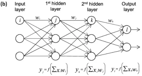
Figure 2.2:Fully connected neural network.
A fully connected neural network is composed by a multiple neurons that are grouped into layers. These layers are stacked subsequently from the input layer to the output layer. Each of them is composed by an arbitrary amount of nodes (neurons), and receives the out-put of the previous layer’s nodes. Then, it propagates its outout-put to all the neurons belonging to the next layer (Figure 2.2). In this way the data flow in a single direction, from input layer to the output layer. In Figure 2.2 you can see a very simple example of a fully connected neural network, with only 2 hidden layers and three neurons for each layer but the output
layer, which has only two neurons. More powerful neural networks are bigger and deeper, i.e. they have more layers and more neurons per layer.
Neurons do not just propagate information, but also process it. Like a neuron in the brain, a node of a neural network receives an input signal and under some conditions, it fires and propagates the signal. In a NN, each neuron receives the output signal from each of the neu-rons it is linked to, it multiplies each signal by a different weight and then sums them together. The result is given in input to a non-linear activation function and its output is propagated to all the following neurons that are linked. There exist different types of activation functions: thesigmoid, thetanh,ReLU (Figure 2.2), etc. The ReLU activation function is fast from a computationally point of view and avoids vanishing gradient problems, present with sig-moid and tanh activation functions. For this reason, ReLU is nowadays state of the art [20].
Figure 2.3:ReLU ac va on func on.
To learn an input-output mapping, neural networks have to adjust the weight matrix, which contains the weights of all the links between the nodes. To do that, we have to give to the model the true output for each input. Then, it is shown we can use techniques like Stochas-tic Gradient Descent (SGD) to change the weights of the model towards to minimize the loss between the predicted output and the true output. If we defineJ as the loss function,θthe set containing all the NN’s weights,xthe training sample and y the training label sampled from the their distributionp, the loss over the whole training set is the following:
J(θ) = Ex,ypˆdataL(x, y, θ) = 1 m m ∑ i=1 L(x(i), y(i).θ) (2.51)
Figure 2.4:Effects of the learning rate on the minimiza on of the loss.
The loss of the gradient with respect to the weightsθcan be defined as:
∇θJ(θ) = 1 m m ∑ i=1 ∇θL(x(i),y (i) θ) (2.52)
Rather than computing the gradient over the whole training set, in SGD it is approximated by using a subset containingm’training samples:
g= 1 m′∇θ m′ ∑ i=1 ∇θL(x(i), y(i), θ) (2.53) The weights are then changed according to: θ← θ−ϵg, whereϵis the learning rate, which progressively decreases during training. In Figure 2.4 it is possible to see the effects of differ-ent learning rates: ifJis defined as the loss of the model andθas the parameters of the model, a too small learning rate requires an infeasible amount of time to learn the task, while a too big one can escape the valley of the local minima.
2.5.2 Convolutional Neural Networks
Figure 2.5:Example of CNN for object classifica on.
CNNs [21] are specialized kind of neural networks that exploits the convolution opera-tion for processing data that have a known grid-like topology. For this reason they can be used for image data. In a fully connected neural network each element of the weight matrix is used exactly once when computing the output of a layer. It is multiplied by one element of the input and then never revisited. In CNNs instead, thanks to the convolution, each mem-ber of the weight matrix, here calledkernel, is used at every position of the input. This does not affect the run-time of the forward propagation but reduces the storage requirements for the model parameters. Most CNN are composed by:
• Convolution layer
• Non-linear activation function • Pooling layer
• Fully-connected layer(s) (usually as output layer)
To be precise, the combination given by Convolution layer, Pooling layer and activation func-tion can be considered as an unique layer; Layers like this are stacked subsequently many times until one or more fully-connected layers at the end of the neural network (Figure 2.5).
Convolution layer
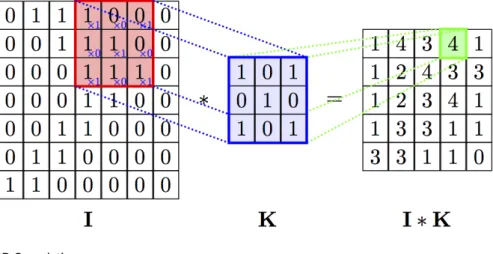
The convolution layer performs a 2D Convolution on the input image: the weight matrix, whose dimension is smaller than the input image and calledkernel, is convolved on the entire input image. Each convolution layer can contain more than a single kernel: in that case we talk about the number of filters of a convolution layer. Each filter can perform a convolution on a different channel of the input image, if it has more than one. The tunable parameters of a Convolution layer are: the dimension of the kernel (on x and y directions), the strides and the padding parameter. The strides are step-size of the shift on both directions of the con-volution operation, i.e. by how many pixels the kernel is shifted on the right and downward in the convolution operation. The padding consists in adding some blank pixels stacked on the borders of the input image in such a way the result of the convolution has the same size of the input image.
Figure 2.6:2D Convolu on.
Non-linear activation function
The output of the convolution layer is one or more matrices (the matrix on the right in Fig-ure 2.6) whose number is equivalent to the number of filters used. Each matrix is the result of the convolution of a filter of the convolution layer with the input of the convolution layer. All the values belonging to those matrices are then passed through a non -linear activation function, like in fully-connected neural networks.
Pooling layer
Figure 2.7:Mean average and max pooling.
The outputs of non-linear activation functions are combined with MaxPooling layers or with AveragePooling operations that summarize statistics of nearby outputs: the matrices that derive from the outputs of the non-linear activation functions are reduced by dimen-sion using an average or the maximum of that region of the original matrices. Figure 2.7 shows how pooling works: a window whose size and strides are decided by the user, shifts along both dimensions of the original matrix, replacing each of the four quadrants with a single value: the maximum or the average of the original values.Pooling helps to make the representation approximately invariant to small translations of the input. Invariance to local translation can be a useful property if we care more about whether some features are present than exactly where they are. Pooling over spatial regions produce invariance to translation, but if we pool over the outputs of separately parametrized convolutions, the features can learn which transformations to become invariant to [21]. Pooling is essential for handling inputs of varying size: to classify images of variable size, the input to the classification layer must have a fixed size.
2.6 Deep Q-Learning
Now that we have briefly explained how neural networks work, we turn back to Q-learning, and in particular to an off-policy temporal difference control. We have said that the equation that governs the action-value function updates is the following:
Q(St, At)←Q(St, At) +α[Rt+1+γmax
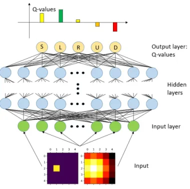
a Q(St+1, a)−Q(St, At)] (2.54) Ideally, the estimation of the value function can be represented in a tabular form, for which an optimal policy can be obtained. However many real-world problems present large or con-tinuous state spaces making training extremely slow. This can be solved by using function approximation methods like neural networks [7]. We refer to a neural network function ap-proximator with weightsθas a Q-network. Remembering that the goal of the agent is to select actions in a way that maximizes cumulative future reward, the objective of the neural network is to approximate the optimal action-value function:
Q∗(s, a) = max
π E[rt+γrt+1+γ
2r
t+2+...|st =s, at=a, π] (2.55) Q∗(s, a)is defined as the maximum expected return achievable by following any policy, after
seeing some sequencesand then taking some actiona,Q∗(s, a) = maxπE[Rt|st =s, at= a, π], in whichπis a policy mapping sequences to actions. A Q-network can be trained by adjusting the parametersθi, at iterationito reduce the mean-squared error in the Bellman equation, where the optimal target valuesr+γmaxa′Q∗(s′, a′)are substituted with ap-proximate bootstrap target valuesy =r+γmaxa′Q(s′, a′;θi−), using parametersθ−i from some previous iteration. This leads to a sequence of loss functionLi(θi)that changes at each iterationi. The Q-learning update at iterationiuses the following loss function:
Li(θi) = E(s,a,r,s’)∼U(D)[(r+γmax
a′ Q(s
′, a′;θ−
i )−Q(s, a;θi))2] (2.56) in whichγis the discount factor determining the agent’s horizon,θi are the parameters of the Q-network at iterationiandθ−i are the network parameters used to compute the target at iterationi. The targets depend on the network weights, differently from supervised learning where are fixed before training begins. During the optimization, the parameters from the previous iterationθ−i are kept fixed when optimizing theith iteration loss functionLi(θi). Differentiating the loss function with respect to the weights, we arrive at the following
gra-dient:
∆θiL(θi) =Es,a,r,s′[(r+γmax
a′ Q(s
′, a′;θ−
i )−Q(s, a;θi))∆θiQ(s, a;θi)] (2.57)
Rather than computing the full expectations, it is common to optimize the loss function by stochastic gradient descent, updating the weights of the neural network at every time step, replacing the expectations using single samples, and settingθ−i =θi−1.
Reinforcement learning is known to be unstable or even to diverge when a nonlinear func-tion approximafunc-tion such as a neural network is used to represent the acfunc-tion-value funcfunc-tion, due to the correlations present in the sequence of observations, the fact that small updates to Q may change the policy and therefore change the data distributions, and the correlations between the action-values (Q) and the target values.
To overcome theses instabilities, two different techniques are used:
• the use of a mechanism calledexperience replaythat randomizes the selection of train-ing samples over the data, removtrain-ing correlations in the observations sequence
• the use of an iterative update that adjusts the action-values (Q) towards target values that are only periodically updated, reducing correlations with the target
At each time-stept, the agent’s experienceet = (st, at, rt, st+1)is stored in a data setDt=
{e1, ..., et}. To perform experience replay, during learning Q-learning updates are applied on samples of experience(s,a,r,s’)∼U(D), drawn uniformly at random from the pool stored samples D. The uniform sampling gives equal importance to all the transitions in the mem-ory replay. More sophisticated sampling strategies that emphasize transitions from which we can learn the most are also possible: they useprioritized memory replays.
The target network parametersθ−i are only updated with the Q-network parameters (θi) ev-ery C steps and are held fixed between individual updates. To be precise, evev-ery C updates we clone the network Q to obtain a target networkQˆand useQˆfor generating the Q-learning
targetsyjfor the following C updates to Q. This modification makes the algorithm more sta-ble compared to standard online Q-learning, where an update that increasesQ(st, at)often also increasesQ(st+1, a), for allaand hence also increases the targetyj, possibly leading to oscillations or divergence of the q-values. Generating the targets using an older set of param-eters adds a delay between the time an update to Q is made and the time the update affects the targetsyj, making divergence or oscillations much more unlikely.
Algorithm 2.1Deep Q-learning with experience replay Initialize memory replay D
Initialize action-value function Q with random weightsθ Initialize target action-value functionQˆwith weightsθ− =θ
forepisode=1,Mdo Initializes1
fort=1,Tdo
Select an actionataccording to the behavior policy
Execute actionatand observe rewardrtand new statest+1
Setst+1 =st
Store transition (st, at, rt, st+1) in D
Sample random minibatch of transitions (sj, aj, rj, sj+1) from D
Setyj =rj +γmaxa′Qˆ(sj+1, a′;θ−)
Perform a gradient descent step on(yj−Q(sj, aj;θ))2w.r.t.θ Every C steps setQˆ =Q
end end
This algorithm is model-free: it solves the RL task directly using samples from the agent experience, without explicitly estimating the reward and transition dynamicsP(r, s′|s, a).
It is also off-policy: it learns about the greedy policya=argmaxa′Q(s, a′;θ), while follow-ing a behavior distribution that ensures adequate exploration of the state space. In practice, the behavior distribution is often selected by anϵ-greedy policy that follows the greedy policy with probability 1-ϵand selects a random action with probabilityϵ.