Javed, Abbas; Larijani, Hadi; Ahmadinia, Ali; Gibson, Des Published in:
IEEE Transactions on Industrial Informatics
DOI:
10.1109/TII.2016.2597746
Publication date: 2017
Document Version Peer reviewed version
Link to publication in ResearchOnline
Citation for published version (Harvard):
Javed, A, Larijani, H, Ahmadinia, A & Gibson, D 2017, 'Smart random neural network controller for HVAC using cloud computing technology', IEEE Transactions on Industrial Informatics, no. 99, pp. 351-360.
https://doi.org/10.1109/TII.2016.2597746
General rights
Copyright and moral rights for the publications made accessible in the public portal are retained by the authors and/or other copyright owners and it is a condition of accessing publications that users recognise and abide by the legal requirements associated with these rights.
Take down policy
If you believe that this document breaches copyright please view our takedown policy at https://edshare.gcu.ac.uk/id/eprint/5179 for details of how to contact us.
Smart Random Neural Network Controller for
HVAC using Cloud Computing Technology
Abbas Javed, Hadi Larijani, Ali Ahmadinia, and Des Gibson
Abstract
Smart homes reduce human intervention in controlling the Heating Ventilation and Air Conditioning (HVAC) systems for maintaining a comfortable indoor environment. The embedded intelligence in the sensor nodes is limited due to the limited processing power and memory in the sensor node. Cloud computing has become increasingly popular due to its capability of providing computer utilities as internet services. In this work, a model for intelligent controller by integrating Internet of Things (IoT) with cloud computing and web services is proposed. The wireless sensor nodes for monitoring the indoor environment and HVAC inlet air, and wireless base station for controlling the actuators of HVAC have been developed. The sensor nodes and base station communicate through RF transceivers at 915 MHz. Random neural network (RNN) models are used for estimating the number of occupants, and for estimating the Predicted mean vote (PMV) based setpoints for controlling the heating, ventilation and cooling of the building. Three test cases are studied (Case 1- data storage and implementation of RNN models on the cloud, Case 2- RNN models implementation on base station, Case 3- distributed implementation of RNN models on sensor nodes and base stations) for determining the best architecture in terms of power consumption. The results have shown that by embedding the intelligence in the base station and sensor nodes (i.e. Case 3), the power consumption of the intelligent controller was 4.4% less than Case 1 and 19.23 % less than Case 2.
Manuscript submitted on May 31, 2015. Revised on June 03,2016. Accepted on July 02, 2016.
Abbas Javed, Hadi Larijani are with the School of Engineering and Built Environment, Glasgow Caledonian University, UK, e-mail: ([email protected].
Ali Ahmadinia is with Department of Computer Science in California State University San Marcos, US.
Des Gibson is with Institute of Thin Films, Sensors and Imaging, Scottish Universities Physics Alliance, University of the West of Scotland
I. INTRODUCTION
Internet of things (IoT) is an emerging technology and has been applied in various applications such as agriculture, healthcare, food monitoring, environmental monitoring, security surveillance, mine safety, building energy management systems (BEMS). Research challenges for deployment of internet of things (IoT) highlighted in [1] are: 1) integrating social networking with IoT solutions, 2) developing green IoT technologies, 3) developing context-aware IoT middleware solutions 4) employing artificial intelligence techniques to create intelligent things of smart objects 5) combining IoT and cloud computing.
There are several functional requirements for BEMS i.e., to measure the environmental pa-rameters (temperature, humidity, light intensity, and CO2), to monitor the energy consumption, feedback from user to maintain the environment according to user requirement, to detect the occupant presence, to learn from the user preferences, to learn the effect of control actions on the environment and to devise the optimal control sequence for energy consumption reduction while maintaining the comfortable indoor environment as per occupant preferences [2].
Due to latest technological developments in wireless communications, low power embedded systems, sensor design and energy storage technology, wireless sensors are replacing the tra-ditional hard wired sensor systems in BEMS. As a result; a new generation of BEMSs have emerged which incorporate wireless sensor networks (WSN) [3]. This integration of WSN in BEMS increases the computer processing, and data storage requirements.
To overcome the problem of high computational processing, data storage and data representation, the authors in [4], integrated the WSN with cloud technologies. The WSNs have limited pro-cessing power, data storage and battery life whereas cloud computing offers greater data storage and processing power. Due to these properties, integration of WSN with cloud computing make a very attractive addition to BEMS.
In this work, a novel RNN based smart controller for HVAC is proposed which incorporates WSN and cloud computing. The smart controller estimates the number of occupants, estimates the predicted mean vote (PMV) based set-points for cooling and heating and learns from user preferences for heating, cooling and ventilation. The environmental data and control parameters are presented on a web platform. The Hybrid Particle Swarm Optimization with Sequential Quadratic Programming (PSO-SQP) [5] has been presented in this paper for training the RNN.
Three test scenarios were compared for determining the best architecture for future BEMS in terms of battery life, and accuracy. The three test case scenarios were:
1) Data storage, data processing and control algorithms were implemented on the cloud. In this scenario, the sensor nodes transmitted the environmental conditions and user preferences to the cloud through base stations. The learning of the RNN algorithm was carried out in the cloud platform and control actions were sent back to the base station to control the actuators.
2) RNN models were trained in the cloud platform and the trained RNN models were imple-mented on the base station. The base station received the information from sensor nodes and estimated the number of occupants, based on this information, the base station took necessary control actions for maintaining a comfortable indoor environment.
3) Data storage, processing and training of RNN was performed on the cloud. The trained RNN model for occupancy was embedded in the sensor nodes for determining the number of occupants. The RNN model for PMV based setpoint estimation and HVAC control were embedded in the base station to take control actions according to the information sent from smart sensor nodes. All three architectures are evaluated in terms of battery life to determine the best suitable architecture for future BEMS.
A. Related Work
In this subsection, a brief overview of different techniques used for BEMS and occupancy estimation techniques is presented. In [6], a low cost WSN based home automation system was proposed in which electrical appliances were controlled through a web server. In [7], the authors presented a smart home energy management system using IEEE 802.15.4 and Zigbee. The smart home energy management system controlled air conditioning, heating, lights and security system by detecting the movement of an occupant. The authors in [8], developed the wireless smart comfort sensing system based on IEEE 1451 standard for monitoring the thermal and indoor air quality of the building. The power consumption for transmitting the data was 60 mW. The authors in [9], implemented the wireless sensor network based distributed sensing and control system for HVAC. The system was decomposed into two modules i.e. radiant cooling module and distributed ventilation model. Both modules were controlled individually for reducing energy consumption.
scheduling method was proposed within the framework of IOT by considering the smart pricing tariffs and user comfort.
BEMS should learn from user preferences in order to reduce energy consumption while main-taining a comfortable indoor environment. This requires feedback from the user through touch screen interfaces, web portals, pc based interfaces, mobile phones etc., [11].
The energy consumption of the building can be improved by 10 to 15% through correct detection of occupancy [12]. The information about the occupancy count can further reduce the energy consumption of the buildings but this requires an accurate system that can detect and give information about the occupancy. The output of Passive infrared (PIR) sensor is binary thus PIR sensors are unable to give the accurate number of people.
In [12], the authors developed an algorithm for occupancy detection by using PIR sensors and reed switches but their sensor platform was unable to count the number of occupants. Occupancy was also estimated by using chair sensors [13]. However, chair sensor was unable to detect a standing occupant in the room.
Humans exhale CO2 during respiration and the measure of CO2 concentration can be used for occupancy estimation, detection, location of occupants, and activity recognition [13]. In [14], the authors exploited the correlation between the CO2 concentration and the occupancy levels. The authors presented occupancy estimation as a deconvolution problem and found that the presented technique was better than artificial neural networks (ANN) and support vector machine (SVM). CO2 sensors give information about Indoor Air Quality (IAQ) . Good IAQ improves the productivity of the occupants inside the building. In [15], the authors compared three different statistical classification models for occupancy detection in an office using information from light, CO2, temperature, and humidity sensors. The accuracy of occupancy detection varied between 95% to 99%. However their work was limited for occupancy detection only (whether the office was occupied or not).
In this work, we developed a smart controller by using multiple RNN models for estimating the occupancy, and for controlling the HVAC. The Hybrid PSO-SQP training algorithm has been used for training the RNN models. Three different architectures of the smart controller were compared to determine the best architecture for getting maximum battery life for the sensor nodes. In section II, a brief description of RNN and the proposed hybrid PSO-SQP training algorithm is given. Followed by a description of system architecture for smart homes in section
III. The RNN models used in the smart controller are described in section IV. The description of different architectures for smart controllers and results are discussed in section V, followed by conclusions in section VI.
II. RANDOMNEURAL NETWORKS
Gelenbe [16] proposed a new class of Artificial Neural Networks (ANN) as Random Neural Networks (RNN) in which signals are either +1 or -1. RNNs can give more detailed system state descriptions because the potential of neuron is represented by integer values rather than binary values [17]. Applications of RNN have been reported for modeling, pattern recognition, image processing, classification, and communication systems [17]. However no such application has been reported so far in implementing control schemes for HVACs in residential/commercial buildings (to the best of our knowledge).
In RNNs, signal travels in the form of impulse between the neurons. If the receiving signal has positive potential (+1) it represents excitation, and if the potential of the input signal is negative (-1) it represents inhibition to the receiving neuron. Each neuron i in the RNN has a state ki(t) which represents the potential at time t. This potential ki(t) is represented by
non-negative integer. If ki(t)>0 then neuron i is in excited state and if ki(t) = 0 then neuron i is
in idle state.
When neuron i is in excited state, it transmits impulse according to the poisson rate ri. The
transmitted signal can reach neuronjas excitation signal with probabilityp+(i, j)or as inhibitory signal with probability p−(i, j), or can leave the network with probability d(i) such that
d(i) + N X j=1 p+(i, j) +p−(i, j)= 1∀i (1) w+(i, j) =rip+(i, j)>0 (2) w−(i, j) =rip−(i, j)>0 (3) combining (1)-(3) r(i) = (1−d(i))−1 N X j=1 w+(i, j) +w−(i, j) (4)
The firing rate between the neuron is represented by r(i) =PN
j=1[w
+(i, j) +w−(i, j)]
. As ’w’
non-negative values. External positive or negative signal can also reach neuron i at Poisson rate Λi and λi respectively. When positive signal is received at neuron i its potential ki(t) will
increase to +1. If neuron i is in excitation state and it receives negative signal the potential of neuron i will decrease to zero. Arrival of negative signal will have no effect on neuron i if its potential is already 0. The description of symbols used is given in Table 1.
Consider the vector K(t)= (k1(t), ...kn(t)) where ki(t) is the potential of neuron i and n is
the total number of neurons in the network. Let K is continuous time Markov process. The stationary distribution of K is represented as:
lim t→∞P r(K(t))) = (k1(t)...kn(t)) = n Y i=1 (1−qi)qiki (5)
For each node i
qi = G+i ri+G−i (6) where G+i = Λi+ N X j=1 qjw+(j, i) (7) G−i = Λi− N X j=1 qjw−(j, i) (8)
w+(j,i) andw−(j,i) are positive and negative interconnecting weights between neurons of jth and ith layer. For input layer I, w+(j,i) and w−(j,i) are equal to zero. Therefore for three layer network qi
for each layer is calculated substituting 7 - 8 in 6, where qi is the probability neuron i excited
at time t.
qiεI =
Λi
ri+λi
where I is input layer (9)
qiεH =
P
iεIqiw+(i, h)
rh +PiεIqiw−(i, h)
where H is hidden layer (10)
qiεO = P iεHqhw +(h, o) rh+ P iεIqhw−(h, o)
A. Hybrid Particle Swarm Optimization with Sequential Quadratic Programming
Majority of researchers have used Gradient Descent (GD) algorithm [18] for learning the weights of RNN models. The GD algorithm is relatively easy to implement but the zigzag behavior may cause it to be stuck near a local minimum for application problems which have multiple local minima. Evolutionary algorithms can be used for solving optimization problems. These techniques are better than gradient base techniques as they do not require calculation of derivatives and they do not get stuck in local minimum (the major problem with GD algorithm). Evolutionary algorithms have been applied for training neural networks. In [19], the authors trained the feed forward neural network with PSO algorithm and found that PSO converges faster than back propagation (BP) algorithm. The PSO algorithm performs well in finding the global minimum but it might be slow to converge to the global minimum. On the other hand, the SQP optimization algorithm [20] can find the optimum weights but in presence of global minima it can get stuck in local minima. The problem of slow convergence of PSO and local minima problem of SQP optimization was addressed by the hybridization of PSO and SQP optimization algorithm in [5]. The Differential Evolution (DE) and Particle Swarm Optimization (PSO) algorithms for training of RNN were implemented in [21] where these algorithms were compared with resilient backpropagation (RPROP) and GD algorithm. The authors showed that for fixed number of epochs, the RPROP algorithm was better than GD algorithm and PSO algorithm achieved higher generalization performance than RPROP algorithm. The goal of training is to learn the input-output relationship by adjusting the interconnection weights. In this paper, we used hybrid PSO-SQP algorithm for RNN training. First, RNN is trained with PSO algorithm to find the global minima, and then based on feasible start point from PSO algorithm, SQP optimization algorithm converges to global minima.
1) Adaptive Inertia Weight-Particle Smarm Optimization Algorithm for RNN: The procedure of applying adaptive inertial weight (AIW) PSO algorithm is as follows
Step1: Initialize a population of S particles with random positions and velocities of d dimen-sions in the problem space. The position vector is an array of interconnected weights of feed forward RNN of I Input nodes, H hidden nodes and O output nodes. The dimensions of D is 2(I.H+H.O). The position vector is formulated as Xsd = [wih+L1w
+L2 ho w −L1 ih w −L2 ho ] where
of [0;1].
w+ihL1 is positive interconnection weight between node i of layer 0 and node h of layer 1.
w+ihL2 is positive interconnection weight between node h of layer 1 and node o of layer 2.
w−ihL1 is negative interconnection weight between node i of layer 0 and node h of layer 1.
w−ihL2 is negative interconnection weight between node h of layer 1 and node o of layer 2. Step2: Each particle from position in generation k moves to new position k+1 by using PSO equation given in 12. Thec1 constant value is set to 2.6 andc2, constant value is set to 1.1.
Step-1:Initialize a population ofSparticles with random positions and velocities ofddimensions in the problem space, represented as (Vsd). The position vector is an array of interconnected weights of feed forward RNN havingI Input nodes,Hhidden nodes andOoutput nodes. The dimensions of
d is 2(I.H+H.O). The position vector is formulated as Xsd = [wih+L1w
+L2 ho w −L1 ih w −L2 ho ] where
1 6 i 6 I, 1 6 h 6 H, 1 6 O 6 O. The weights are randomly distributed over the interval of [0;1].
Step-2: Each particle from position in generation k moves to new position k+1 by using PSO equation given in equation 12. The c1 constant value is set to 2.6 and c2, constant value is set
to 1.1. Vsdk+1 =W Vsdk +c1rand()(Pbestsdk −X k sd)+ c2rand()(Gkbestsd −X k sd) (12) Xsdk+1 = Xsdk +Vsdk+1 (13) where Pbestsd, Gbestsd are the local best for position vector Xsd and global best for vector
Xsd.
Wsdk = 1 − 1
1 +exp(−α.ISAksd) (14)
where α is a constant with values in between 0 to 1 and ISAksd is given as:
ISA= 1− X k sd −P k best Pk bestsd −Gkbestsd +ε (15)
where ε is a small position constant. Step-3: For each particle, evaluate the fitness function
E = 1 2 N X p=1 O X o=1 [qo(p)−qdes,o] 2 (16)
Initialize the random neural network with random interconnected weights
Xsd =[wij +L1 wij +L2 wij -L1 wij -L2 ]
Train the network with PSO algorithm
If PSO training finished NO
Store the weights YES
Train the network with SQP optimization algorithm
If training finished NO
Store the weights YES
Fig. 1. Flow chart of Hybrid PSO-SQP
where N is the number of patterns, O is the number of output, qdes,o is the desired output in training pattern, qo(p) is the output of RNN calculated by solving equations (9-11).
Step-4: Compare particle fitness evaluation with particle local best Pbest. If current fitness evaluation value is less than Pbest, then update Pbest to current value and the Pbest location equal to current location in d dimensional space.
Step-5: Compare fitness evaluation with all Pbest of population S. If Pbest is less than Gbest update Gbest to the current particle’s array index.
Step-6: Compute the average squared error. If the MSE is not less than threshold, go to Step-2. If the stopping criteria is met or maximum number of iterations is reached, learning is complete. In this work, RNN is trained with AIW-PSO algorithm for 100 iterations. After finishing 100 iterations, the weights of RNN are optimized using SQP optimization algorithm. The flow chart of AIW-PSO algorithm is shown in Fig 1.
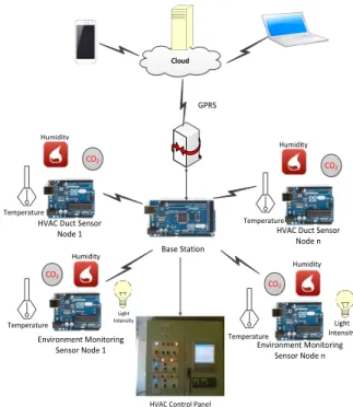
CO2 Environment Monitoring Sensor Node 1 Humidity CO2 Temperature Temperature Humidity Light Intensity CO2 CO2
HVAC Duct Sensor Node n Humidity Temperature Temperature Humidity Environment Monitoring Sensor Node n HVAC Duct Sensor
Node 1 Cloud Base Station GPRS Light Intensity
HVAC Control Panel
Fig. 2. System Architecture for Smart Home
III. SYSTEM ARCHITECTURE FORSMARTHOME
The system architecture of smart home is given in Fig 2. The system consists of sensor nodes for monitoring the indoor environment, HVAC duct sensor node, the base station is connected with the workstation through serial port and web portal for display.
A. Environment Sensor node
Each room has one environment sensor node. The sensor node measures temperature, humidity, and CO2. Sensor nodes were built with Arduino UNO boards which have 2KB RAM and
32KB of program memory. Each sensor node is connected with RF transceiver (RFM 69W) and communicating with the base station at 915 MHz. Sensor nodes were also developed with Moteino R4 [22] which is low power clone of Arduino UNO board. A DHT 22 sensor was used to measure temperature and humidity, a COZIR CO2 sensor [23] was used to measure CO2
B. HVAC Duct Sensor node
Each room has one HVAC duct sensor node. A sensor node measures temperature, humidity, CO2 for the inlet air coming inside the room from the HVAC. The HVAC duct sensor node was
built with the same board and RF transceiver as used for environment sensor nodes. The HVAC duct sensor node is also developed with using MOTEINO R4 board.
C. Base Station
The base station was implemented by using Arduino Mega 2560 board which has 8KB RAM and 256 KB of program memory. The board is connected with RFM 69W transceiver and it receives information from the sensor nodes and transfers the data to the workstation through serial port. The base station controls the environment of the chamber by controlling the actuators of the HVAC.
D. Server for RNN training and data storage
To create the cloud processing scenarios, the base station was connected with the workstation through serial port. The base station transmitted the data received from the sensor nodes to the workstation which stored the data and trained the RNN by using PSO-SQP algorithm. Apart from this it also uploaded the environmental parameters/control signals on the cloud computing platform, ThingSpeak [24].
IV. RNNMODELS FOR INTELLIGENTCONTROL OFBUILDING
The smart control of the building was managed by using three different RNN models. The description of each RNN model is given in the following sub sections.
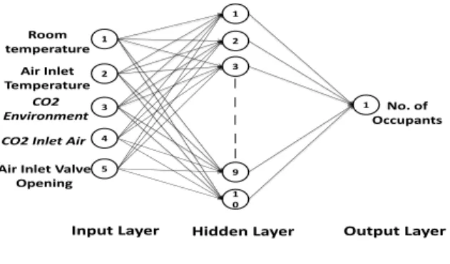
A. Occupancy Estimation
A RNN model was trained to learn the relationship between the occupancy levels and CO2
con-centrations, room temperature, and ventilation actuation signals for identification of occupancy estimation model. The inputs for RNN model were: room temperature, inlet air temperature, inlet CO2 concentration, indoor CO2 levels, and inlet air actuation signal while output of RNN
model was occupancy levels. The RNN model for occupancy estimation is shown in Fig 3. The effect of outside temperature on determining the number of occupants was negligible as an
CO2 Environment Air Inlet Temperature Room temperature
Air Inlet Valve Opening 1 2 3 1 2 1 3 1 0 9
Input Layer Hidden Layer Output Layer
No. of Occupants 4
5
CO2 Inlet Air
Fig. 3. Occupancy Estimator
HVAC was maintaining the heating/cooling setpoints for the building. The rise/decline in the indoor temperature of the building due to outside temperature was controlled through HVAC. Therefore, the effect of the outside temperature on the building was indirectly reflected by the change in HVAC inlet air temperature.
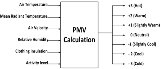
B. PMV based setpoint estimator
Thermal comfort is state of mind when a person is satisfied with indoor environment of the building. Human body decides the level of thermal comfortably with the amount of heat exchange between the body and environment. Thermal comfort can be different for different people wearing different types of clothing. For calculating thermal comfort in buildings, Predictive Mean Vote (PMV) method was used. PMV is the most commonly used indoor thermal comfort index in buildings [25]. Fanger developed the thermal sensation scale of 7 values to determine the thermal comfort index. PMV was developed as a function of six variables: air temperature, mean radiant temperature, air velocity, air humidity, clothing resistance, and activity level as shown in Fig 4. Where PMV=0 means Neutral, PMV =1 represents Slightly Warm environment, PMV=-1 represents slightly Cool indoor environment. Similarly if the user selects PMV=-0.7, it means the indoor environment is near to slightly cool index. As per ISO recommendation, it is required to maintain PMV at 0 with tolerance of 0.5.
In this work, the training data set was generated by using Fanger equation for PMV [25]. In order to reduce the human interference, clothing insulation of 0.8, metabolic rate of 1.1, and air velocity of 0.15 m/s were assumed to be constant. After generating the training dataset, RNN
PMV Calculation
Air Temperature Mean Radiant Temperature Air Velocity Relative Humidity Clothing Insulation Activity level +3 (Hot) +2 (Warm) +1 (Slightly Warm) 0 (Neutral) -1 (Slightly Cool) - 2 (Cool) - 3 (Cold)
Fig. 4. PMV Thermal Sensation Scale
was trained with PMV and humidity as inputs and temperature as an output. A 2-4-1 RNN was trained with hybrid PSO-SQP training algorithm. In this work, PMV of -0.1,-0.3,-0.5 was tested for heating setpoint and PMV of 0.3, 0.5 and 0.7 was tested for cooling set point.
C. HVAC Control
A smart RNN controller was trained for maintaining comfortable indoor environment by controlling the heating, cooling and ventilation of HVAC. The cooling set points and heating set points were varied by occupants to train the controller. A 5-7-3 RNN controller with 5 neurons as input, 7 neurons in the hidden layer and 3 neurons as output layer (shown in Fig 5) was trained with PSO-SQP training algorithm. The training dataset for the RNN HVAC controller was collected by manually operating the HVAC for maintaining the heating setpoints of 19 oC, 20 oC, 21 oC, 22 oC, 23oC and cooling setpoints of 25 oC, 26 oC, 27 oC, 28 oC. The accuracy of RNN HVAC controller was calculated in percentages by comparing the output of trained RNN with the training dataset. The smart controller learned the human preferences with accuracy of 94.87% for heating, 98.39% for cooling, and 99.27% for ventilation.
V. RESULTS ANDDISCUSSION
The intelligent controller was tested for controlling heating, cooling and ventilation in the environment chamber.
A. Test Bed
The test bed consists of an environment chamber of 12x8x8 ft located in Glasgow Caledo-nian University campus. The test chamber has dedicated HVAC that can humidify/dehumidify,
1 2 3 1 2 1 4 3 6 5 7
Input Layer Hidden Layer Output Layer
Heating Cooling Error Cooling Setpoint Heating Setpoint 4 Heating Error 5 CO2 2 Cooling 3 Ventilation
Fig. 5. RNN HVAC controller
Fig. 6. Indoor View of Environment Chamber
heat/cool the environment chamber. The chiller of the environment chamber can bring the air temperature down to 5 oC. Inside the environment chamber, there are two sensor nodes one for HVAC duct and one for monitoring the environment of the chamber. The base station is connected with control panel of the environment chamber to turn on/off heater, cooler and ventilation. The indoor view of the environment chamber is shown in Fig 6.
B. Occupancy Estimation
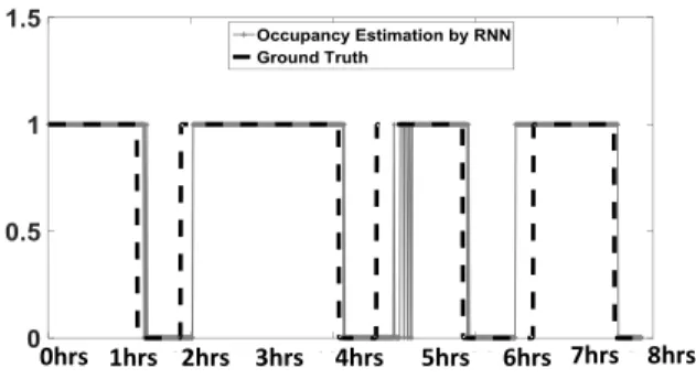
The RNN model for occupancy estimation was tested in the environment chamber for detecting a single occupant. The ground truth value for occupancy was recorded manually in the sensor node for generating the training dataset. The smart controller detected the occupancy with an accuracy of 87.4% as shown in Fig 7.
1hrs 2hrs 3hrs 4hrs 5hrs 6hrs 7hrs 8hrs 0hrs
Fig. 7. Occupancy Estimation with RNN Occupancy Estimator
0hrs 1hrs 2hrs 3hrs 4hrs 5hrs 6hrs 7hrs 8hrs
Fig. 8. Occupancy Estimation with RNN Occupancy Estimator
The study was carried out to check the performance of RNN for estimating the occupancy when the chamber was occupied up to three persons. The CO2 concentrations increased when
number of occupants increased but when the occupants left the chamber, the CO2 concentrations
remained constant for a long period of time. This non-linear behaviour makes the occupancy estimation a very challenging task. The occupancy estimation by RNN is shown in Fig 8. The accuracy of RNN occupancy estimation was 92.48% and with an error of 3.81% for estimating +/- 1 person to the ground truth values.
C. HVAC control
The user can maintain the PMV based setpoints for heating and cooling by using RNN PMV based setpoint estimator or if not satisfied with the PMV based setpoints, the air temperature of the building can be maintained according to the user requirement. The upper and lower threshold for turning ON/OFF the heating/cooling of the environment chamber was implemented. The
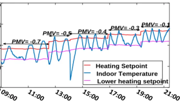
PMV based indoor air temperature of the environment chamber along with PMV based heating setpoints, and lower threshold of heating setpoints is shown in Fig 9. The indoor air temperature along with PMV based cooling setpoint and lower cooling setpoint is shown in Fig 10. To test the performance of the RNN controller, the PMV based setpoints for heating were varied to check the heating control. The HVAC cooling control was tested by turning ON the heating to allow the air temperature of the environment chamber to reach the cooling setpoint. Once cooling setpoint was reached, the HVAC cooling was turned ON as shown in Fig 10. The maximum overshoot for maintaining the PMV based heating setpoint was 0.69 oC while for PMV based cooling setpoint, the maximum overshoot was 0.21 oC. The amount of time in terms of percentages when overshoot was above 0.5 oC was 2.75%.
The smart controller was also tested for maintaining the user defined heating setpoints (19 oC, 20 oC , 21 oC , 22 oC , and 23 oC ) during winters and for maintaining the cooling setpoints (25 oC, 26 oC , 27 oC , and 28 oC) during summer season. The indoor air temperature while maintaining heating setpoints is shown in Fig 11 and the indoor air temperature for maintaining cooling setpoints is shown in Fig 12. The maximum overshoot for maintaining heating and cooling setpoints during summers was 0.3oC.
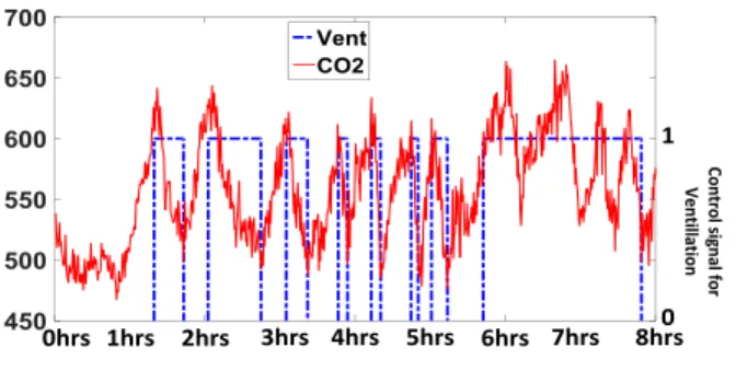
The smart controller turns on the ventilation of the environment chamber if CO2 level reaches
600 PPM and ventilation remained ON until CO2 levels dropped to 500 PPM. The performance
of controlling the ventilation of the test chamber is shown in Fig 13. The RNN HVAC controller and RNN PMV based setpoint estimator was trained during the month of February, while the tests were also conducted during summers as well and from Fig 12 it is shown that the smart controller can maintain accurate temperature during summers as well. Moreover RNN HVAC controller was trained for maintaining user defined setpoints but results showed that it could maintain accurate temperature for PMV based setpoints as well.
D. Comparison of Training algorithms for RNN
The PSO-SQP training algorithm was compared with PSO and GD training algorithm for training occupancy estimator, PMV based setpoint estimator and HVAC control. The MSE with all training algorithms is shown in Table I. The MSE of PSO-SQP training algorithm was 63.52% less than GD and 35.52% less than PSO for occupancy estimator. The MSE of PSO-SQP training algorithm was 71.50% less than GD and 63.23% less than PSO for training the
0 100 200 300 400 500 600 18 20 22 24 26 Heating Setpoint Indoor Temperature Lower heating setpoint
PMV= -0.7 PMV= -0.4 PMV= -0.3 PMV= -0.1 PMV= -0.5 11:00 13:00 15:00 17:00 19:00 21:00 09:00
Fig. 9. . Indoor Air Temperature alongwith heating setpoints, yaxis represents temperature in celsius while x-axis represents the time samples after every 1 min.
10:0011:0012:0013:0014:0015:0016:0017:0018:0019:0020:00
Fig. 10. Indoor Air Temperature alongwith cooling setpoints, yaxis represents temperature in celsius while x-axis represents the time samples after every 1 min
08:0009:00 11:00 13:00 15:00 17:00 19:00 21:00
Fig. 11. . Indoor Air Temperature alongwith heating setpoints of 19oC, 20oC, 21oC,22oC,23oC, yaxis represents temperature in celsius while x-axis represents the time samples after every 1 min
11:0012:0013:0014:0015:0016:0017:0018:0019:0020:00
Fig. 12. Indoor Air Temperature alongwith cooling setpoints of 25oC, 26oC,27oC, 28oC, y-axis represents temperature in celsius while x-axis represents the time samples after every 1 min
1 0 Co n tro l s ig n al fo r V en til la tio n 1hrs 2hrs 3hrs 4hrs 5hrs 6hrs 7hrs 8hrs 0hrs
Fig. 13. Ventilation testing- left yaxis represents the CO2concentration in ppm - right yaxis represents the Ventilation ON/OFF
signal
TABLE I. COMPARISON OFMSEFORTRAINING ALGORITHMS
Algorithm Occupancy Estimator HVAC Control Setpoint Estimator
GD 4.03e-02 9.02e-02 2.63e-05
PSO 2.28e-02 6.99e-02 1.67e-05
PSO-SQP 1.47e-02 2.57e-02 6.11e-06
HVAC control. Similarly for PMV based setpoint estimator, the MSE of PSO-SQP training algorithm was 76.76% less than GD and 63.41% less than PSO. The results showed that hybrid PSO-SQP training algorithm for RNN outperformed GD and PSO algorithm in terms of MSE.
E. Case Study to determine the best architecture for embedding the RNN controller for getting maximum battery life
In this study, we tested three different architectures for smart controller to determine the best architecture for maximum battery life.
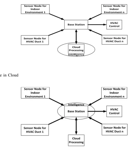
1) Case 1 : Processing in Cloud: Data storage, data processing and control algorithm were implemented on the cloud. In this scenario, the sensor nodes transmitted the environmental conditions and user preferences to cloud through base station and the control actions were determined by base station by using cloud processing. The architecture is shown in Fig 14. The Base station requires only 12004 bytes for program memory and RAM consumption was 1050 bytes
2) Case 2: Control Algorithm at Base Station: Data storage and processing on the cloud while control algorithm was implemented on the base station. In this scenario, the model was trained on
Base Station Sensor Node for
Indoor Environment 1
Sensor Node for Indoor Environment n
Sensor Node for HVAC Duct 1
Sensor Node for HVAC Duct n HVAC Control Cloud Processing Intelligence
Fig. 14. Intelligence in Cloud
Base Station Sensor Node for
Indoor Environment 1
Sensor Node for Indoor Environment n
Sensor Node for HVAC Duct 1
Sensor Node for HVAC Duct n HVAC Control Cloud Processing Intelligence
Fig. 15. Intelligence in Base station
the cloud platform and the trained RNN models were implemented on the base station. The base station received the information from sensor nodes and estimated the number of occupants, based on this information the base station took necessary control actions for maintaining a comfortable indoor environment. The architecture is shown in Fig 15.
3) Case 3: Base Station with Intelligent Sensor Nodes : Data storage and processing on cloud with embedded intelligence in sensor nodes and base station. In this scenario, the sensor nodes had embedded intelligence for determining the number of occupants and base station took control actions according to the information sent from smart sensor nodes. The architecture of this scenario is given in Fig 16.
4) Comparison of Architectures: The base station of Case 1 consumed 21.34 % less RAM, 44% less program memory and 18.40% less power compared to base station of Case 2. As compared to base station of Case 3, the base station of Case 1 required 35.42% less memory, 16.335%
Base Station
Sensor Node for Indoor Environment n
Sensor Node for HVAC Duct 1
Sensor Node for HVAC Duct n HVAC Control Cloud Processing Intelligence Intelligence Sensor Node for
Indoor Environment n
Intelligence
Fig. 16. Intelligence in Base station and Sensor Node
less RAM but consumed 8.22% more energy. The sensor node for Case 1 required 32.42% less program memory, 28.28% less RAM and 21.42% less power consumption as compared to the Case 3. The detailed comparison of the resources, power consumption is given in Table II while comparison of power consumption is shown in Fig 17. The arduino UNO board was not suitable for implementing the sensor node due to its high power consumption, so a similar node was implemented with another lower power board (Moteino R4) which hadthe same Atmel 328P microcontroller. The battery life for this sensor node was 98 days. The base station for Case 2 required 79.42%
The base station for Case 2 requires 79.42% more program memory, 27.14% more RAM, and 22.55% more power consumption as compared to base station of Case 1. Similarly as compared to base station of Case 3, it requires 15.85% more program memory, 6.375% more RAM and 32% more power consumption. The sensor node for this scenario is same as used in Case 1. The base station for Case 2 required 79.42% more program memory, 27.14% more RAM, and 22.55% more power compared to base station of Case 1. Similarly as compared to base station of Case 3, it required 15.85% more program memory, 6.375% more RAM and 32% more power. The sensor node for this scenario was the same used in Case 1. The base station of Case 3 required 54.84% more program memory, 19.52% more RAM and 7.6% less power than base station of Case 1.
The base station of Case 3, required 13.697% less program memory, 5.99% less RAM and 24.60% less power than base station of Case 1. But the intelligent sensor node consumed 27.78% more power than the standard sensor node. The MOTEINO low power sensor node
TABLE II. COMPARISON OFPOWERCONSUMPTION Power Con-sumption Program Memory Require-ments RAM Available Battery Life Control Deci-sion Delay Base Station for Case 1 465.55 mW 12004 bytes 1050 bytes 264.46 hrs 350ms Base Station for Case 2 570.45 mW 21538 bytes 1335 bytes 215.82 hrs 8.5ms Base Station for Case 3 430.05 mW 18588 bytes 1255 bytes 286.28 hrs 7.0ms Arduino Sen-sor Node for Case 1 & Case 2 388.8 mW 12984 bytes 753 bytes 316.66 hrs N/A Arduino Sen-sor Node for Case 3 497.52 mW 19214 bytes 1050 bytes 247.46 hrs N/A Moteino Sen-sor Node for Case 1 & Case 2 29.08 mW 13302 bytes 783 bytes 2352.13 hrs N/A Moteino Sen-sor Node for Case 3 32 mW 18150 bytes 1097 bytes 2137 hrs N/A
with embedded intelligence consumed 10.01% more power than the similar MOTEINO low power sensor node without intelligence. The battery life for this sensor node was 89 days. The overall power consumption (base station and sensor node) for Case 3 was 4.4% less than the Case 1 and 23.82% less than Case 2. In terms of power consumption, Case3 is the best architecture for getting maximum battery life.
The time taken for control decision by base station in all three architectures was also calculated. The base station for Case 1 took an average time of 350 ms. The minimum time taken by base station was 295 ms while the maximum time was 995ms. The base station was monitoring the environment every 1 minute so this delay of control decision had no effect on the performance of the controller. The time required for base station in Case 2 was 8.7ms and in Case 3 was 7.0ms.
Fig. 17. Comparison of Power Consumption , y-axis represents the power in mW
VI. CONCLUSION
In this work, we presented our novel RNN based intelligent controller for HVAC control. The RNN controller calculates the number of occupants, estimates the predicted mean vote based setpoints for heating and cooling, and learns the user preferences for controlling heating, cooling and ventilation. The occupancy estimation was 92.48% accurate with an error of 3.81% for estimating +/- 1 person. The training of RNN models was performed by our novel hybrid PSO-SQP training algorithm. The results showed that PSO-SQP training algorithm gives 76.76% less MSE compared to GD training algorithm. The power consumption of the sensor nodes is a major hurdle in using IoT. Three different architectures for intelligent control of the building was presented and evaluated in terms of battery life and control decision delay. The sensor node with embedded intelligence consumed 10.01% more energy than standard sensor node but overall power consumption (base station and sensor nodes) for Case 3 (control algorithm on base station with intelligent sensor node for occupancy) was 4.4% less than the Case 1 ( control algorithm on cloud). In terms of control decision delay, Case 3 outperformed other architectures. The control decision delay of Case 3 is 7.0 ms.
REFERENCES
[1] L. Da Xu, W. He, and S. Li, “Internet of things in industries: A survey,”IEEE Transactions on Industrial Informatics, vol. 10, no. 4, pp. 2233–2243, 2014.
[2] A. D. Paola, M. Ortolani, G. L. Re, G. Anastasi, and S. K. Das, “Intelligent management systems for energy efficiency in buildings: A survey,”ACM Computing Surveys (CSUR), vol. 47, no. 1, p. 13, 2014.
[3] A. H. Kazmi, M. J. O’grady, D. T. Delaney, A. G. Ruzzelli, and G. M. O’hare, “A review of wireless-sensor-network-enabled building energy management systems,”ACM Transactions on Sensor Networks (TOSN), vol. 10, no. 4, p. 66, 2014.
[4] W. Kurschl and W. Beer, “Combining cloud computing and wireless sensor networks,” in Proceedings of the 11th International Conference on Information Integration and Web-based Applications & Services. ACM, 2009, pp. 512–518.
[5] T. A. A. Victoire and A. E. Jeyakumar, “Hybrid pso–sqp for economic dispatch with valve-point effect,”Electric Power Systems Research, vol. 71, no. 1, pp. 51–59, 2004.
[6] A. Z. Alkar and U. Buhur, “An internet based wireless home automation system for multifunctional devices,”Consumer Electronics, IEEE Transactions on, vol. 51, no. 4, pp. 1169–1174, 2005.
[7] D.-M. Han and J.-H. Lim, “Smart home energy management system using ieee 802.15. 4 and zigbee,”IEEE Transactions on Consumer Electronics, vol. 56, no. 3, pp. 1403–1410, 2010.
[8] A. Kumar and G. P. Hancke, “An energy-efficient smart comfort sensing system based on the ieee 1451 standard for green buildings,”IEEE Sensors Journal, vol. 14, no. 12, pp. 4245–4252, 2014.
[9] C. Li, Z. Li, M. Li, F. Meggers, A. Schlueter, and H. B. Lim, “Energy efficient hvac system with distributed sensing and control,” in Distributed Computing Systems (ICDCS), 2014 IEEE 34th International Conference on. IEEE, 2014, pp. 429–438.
[10] J. Serra, D. Pubill, A. Antonopoulos, and C. Verikoukis, “Smart hvac control in iot: Energy consumption minimization with user comfort constraints,”The Scientific World Journal, vol. 2014, 2014.
[11] H. Hagras, F. Doctor, V. Callaghan, and A. Lopez, “An incremental adaptive life long learning approach for type-2 fuzzy embedded agents in ambient intelligent environments,”Fuzzy Systems, IEEE Transactions on, vol. 15, no. 1, pp. 41–55, 2007.
[12] Y. Agarwal, B. Balaji, R. Gupta, J. Lyles, M. Wei, and T. Weng, “Occupancy-driven energy management for smart building automation,” inProceedings of the 2nd ACM Workshop on Embedded Sensing Systems for Energy-Efficiency in Building. ACM, 2010, pp. 1–6.
[13] T. Labeodan, W. Zeiler, G. Boxem, and Y. Zhao, “Occupancy measurement in commercial office buildings for demand-driven control applicationsa survey and detection system evaluation,”Energy and Buildings, vol. 93, pp. 303–314, 2015.
[14] A. Ebadat, G. Bottegal, D. Varagnolo, B. Wahlberg, and K. H. Johansson, “Regularized deconvolution-based approaches for estimating room occupancies,”IEEE Transactions on Automation Science and Engineering, vol. 12, no. 4, pp. 1157–1168, 2015.
[15] L. M. Candanedo and V. Feldheim, “Accurate occupancy detection of an office room from light, temperature, humidity and co 2 measurements using statistical learning models,”Energy and Buildings, vol. 112, pp. 28–39, 2016.
[16] E. Gelenbe, “Random neural networks with negative and positive signals and product form solution,”Neural computation, vol. 1, no. 4, pp. 502–510, 1989.
[17] S. Timotheou, “The random neural network: a survey,”The computer journal, vol. 53, no. 3, pp. 251–267, 2010.
[18] E. Gelenbe, “Learning in the recurrent random neural network,”Neural Computation, vol. 5, no. 1, pp. 154–164, 1993.
[19] K. Chau, “Particle swarm optimization training algorithm for anns in stage prediction of shing mun river,”Journal of hydrology, vol. 329, no. 3, pp. 363–367, 2006.
[20] W. Hock and K. Schittkowski, “A comparative performance evaluation of 27 nonlinear programming codes,”Computing, vol. 30, no. 4, pp. 335–358, 1983.
[21] M. Georgiopoulos, C. Li, and T. Kocak, “Learning in the feed-forward random neural network: A critical review,”
Performance Evaluation, vol. 68, no. 4, pp. 361–384, 2011.
[22] “Moteino R4,” https://lowpowerlab.com/moteino/, 2015, [Online; accessed 21-May-2015].
[23] D. Gibson and C. MacGregor, “A novel solid state non-dispersive infrared co2 gas sensor compatible with wireless and portable deployment,”Sensors, vol. 13, no. 6, pp. 7079–7103, 2013.
[24] “ThingSpeak, Internet of Things,” https://thingspeak.com, 2015, [Online; accessed 21-May-2015].
[25] P. Fanger, “Thermal comfort: analysis and applications in environmental engineering,” 1972.
Abbas Javed received his BSc. degree in Computer Engineering from COMSATS Institute of Information Technology (CIIT), Pakistan in 2006 and MSc degree in Control Systems from The University of Sheffield, UK in 2008. In 2009-2012, he worked as Lecturer in Department of Electrical Engineering, CIIT. He received his PhD degree from Glasgow Caledonian University in 2016. His current research interests are in embedded systems, IoT, cloud computing, indoor thermal comfort and machine learning.
Professor Hadi Larijani received his Ph.D. in Computer Science from Heriot-Watt Univ. Edinburgh, UK in 2006. He is a Professor of Computer Networks and Intelligent Systems in the Department of Computer, Communications and Interactive Systems in the School of Engineering and Built Environment. He has extensive experience in wireless communications, sensors, RF-harvesting, intelligent systems, performance evaluation of computer systems and networks, computer network simulation, software engineering, VoIP, LTE, Cognitive Radio, Building Energy management systems and intelligent software agents. His work has resulted in over 60 international journals, patents, and conference publications; he has also been awarded as principal investigator over 1 million pounds worth of grants.
Ali Ahmadinia received his Ph.D. degree from University of Erlangen-Nuremberg, Germany, in 2006. In 2004-2005, he worked as a research associate in Electronic Imaging Group, Fraunhofer Institute - Integrated Circuits (IIS), Erlangen, Germany. In 2006-2008, he was a research fellow in the School of Engineering and Electronics, University of Edinburgh, UK. In 2008, he joined Glasgow Caledonian University, UK, where he was a senior lecturer in embedded systems. He is currently a faculty member of Department of Computer Science in California State University San Marcos, US. His research has resulted more than 100 international journal and conference publications in the areas of recongurable computing and system-on-chip design, wireless and DSP applications.
Professor Des Gibson holds a BSc (hons 1st class) physics and a PhD in thin film optics, both from the Queen‘s University, N Ireland. He has a thirty year track record in industry, academic based research & development and successful physics based product commercialisation, gained globally with technical and managing director roles within blue chip organizations, small to medium sized companies, start-ups and close associations with academia. He has co-founded four physics based technology companies focussing on thin film & sensor technologies and remains a director of two; Gas Sensing Solutions Ltd co-founded 2006 and a recent winner of an Institute of Physics Innovation Award 2014 and also Applied Multilayers Inc, co-founded 2002. Motivated by fresh challenges and a desire to focus on research, September 2014 he joined the University of the West of Scotland as professor in thin film & sensor technologies and is director of the Institute of Thin Films, Sensors & Imaging. Des is a chartered engineer and physicist (CEng & CPhys), Fellow of the Institute of Physics (FInstP), senior member of the Optical Society of America and a named inventor on thirteen patents with over eighty technical publication and articles in thin films, sensors and optoelectronics.