A statistical approach to provide explainable convolutional neural network parameter optimization

(1)

Research Online

ECU Publications Post 2013

1-1-2019

A statistical approach to provide explainable convolutional neural

network parameter optimization

Saman Akbarzadeh

Edith Cowan University, [email protected]

Selam Ahderom

Kamal Alameh

Follow this and additional works at: https://ro.ecu.edu.au/ecuworkspost2013 Part of the Engineering Commons

10.2991/ijcis.d.191219.001

Akbarzadeh, S., Ahderom, S., & Alameh, K. (2019). A statistical approach to provide explainable convolutional neural network parameter optimization. International Journal of Computational Intelligence Systems, 12(2), 1635-1648.

https://doi.org/10.2991/ijcis.d.191219.001

This Journal Article is posted at Research Online. https://ro.ecu.edu.au/ecuworkspost2013/7516

(2)

Vol.12(2), 2019,pp.1635–1648

DOI:https://doi.org/10.2991/ijcis.d.191219.001; ISSN: 1875-6891; eISSN: 1875-6883

https://www.atlantis-press.com/journals/ijcis/

A Statistical Approach to Provide Explainable Convolutional

Neural Network Parameter Optimization

Saman Akbarzadeh*, Selam Ahderom, Kamal Alameh

Electron Science Research Institute, Edith Cowan University, JO23.241, 270 Joondalup Drive, Joondalup, Western Australia 6027, Australia

A R T I C L E I N F O Article History Received 27 May 2019 Accepted 16 Dec 2019 Keywords Optimization

Convolutional neural network Hyperparameter

Design of experiment Taguchi

Deep learning

A B S T R A C T

Algorithms based on convolutional neural networks (CNNs) have been great attention in image processing due to their ability to find patterns and recognize objects in a wide range of scientific and industrial applications. Finding the best network and opti-mizing its hyperparameters for a specific application are central challenges for CNNs. Most state-of-the-art CNNs are manually designed, while techniques for automatically finding the best architecture and hyperparameters are computationally intensive, and hence, there is a need to severely limit their search space. This paper proposes a fast statistical method for CNN parameter optimization, which can be applied in many CNN applications and provides more explainable results. The authors specifically applied Taguchi based experimental designs for network optimization in a basic network, a simplified Inception network and a simplified Resnet network, and conducted a comparison analysis to assess their respective performance and then to select the hyperparameters and networks that facilitate faster training and provide better accuracy. The results show that up to a 6% increase in classification accuracy can be achieved after parameter optimization.

1. INTRODUCTION

Convolutional neural networks (CNNs) have been widely used for image recognition [1], including hyperspectral data classifi-cation [2] and video classificlassifi-cation [3]. Reducing the architecture size of CNNs, in term of their particular task and dataset, makes them more attractive for use in mobile phones and embedded sys-tems, where less power consumption and overall cost reduction are crucial factors [4–8]. To date, designing state-of-the-art CNN algorithms for specific datasets, such as images, has been time-consuming (manually engineered) and computationally intensive [8–13]. Some techniques have been proposed for automatically designing CNNs, however, these techniques either require huge computational resources or do not match manually-engineered accuracies [14–18]. In addition, for many applications, the com-plexity of automatically designed CNN algorithms render them neither interpretable nor explainable enough to be used safely [19,20]. Using a statistical approach to optimize the performance of CNN models not only helps build optimum networks accord-ing to required criteria, but also makes models more explainable. Statistical experimental designs have been widely applied to vari-ous optimization problems [21–23] including parameter optimiza-tion of perceptron neural networks [24–26]. However, for proper optimization of the hyperparameters of deep learning networks, the design of experiment (DOE) is powerful technique, and, to

*_{Corresponding author. Email: [email protected]}

our knowledge, this has never been investigated. In this paper, we propose DOE algorithms based on applying Taguchi statistical methods [27] for optimizing CNN parameters, whereby spectral agricultural data is evaluated using three simplified CNN architec-tures. Finally, to validate our new approach the results are compared with award-winning CNN architectures.

2. EXPERIMENTAL METHODS

The proposed primitive cells that are the building blocks of the proposed CNN network, are described and compared with those used in current state-of-the-art conventional CNN network archi-tectures. Next, the Taguchi method is introduced with four exper-iments conducted to optimize the various parameters of the CNN network.

2.1. The Convolutional Neural Network

Primitives

Most CNNs require huge memory and computational resources. Therefore, the size of the CNN becomes important for applica-tions running on limited resources (e.g., limited speed and memory of mobile phones). In this study, in order to build up an efficient CNN network, primitive blocks from well-known CNN architec-tures have been adapted and used, namely, the VGG network, the Inception network, and the Resnet network [10,11,13].

(3)

2.1.1. Simple primitive block

The simple primitive block of the proposed CNN was designed to include a convolutional layer with batch normalization, Recti-fied Linear Unit (ReLu) function, and max pooling. The advantage of using ReLu instead of traditional neural network functions, like sigmoid or hyperbolic functions, is that training is typically faster. The ReLu formula is f(x) = max (0, x) [27]. The batch normal-ization, which is normalization of the network’s weights in each layer, has many advantages, including faster learning rate conver-gence, efficient weight initialization, and additional regularization, all of which result in faster training with lower overfitting [28]. Max pooling reduces the computation by extracting the most impor-tant features from a kernel, thereby producing a smaller feature representation [29,30].

2.1.2. The Inception primitive blocks

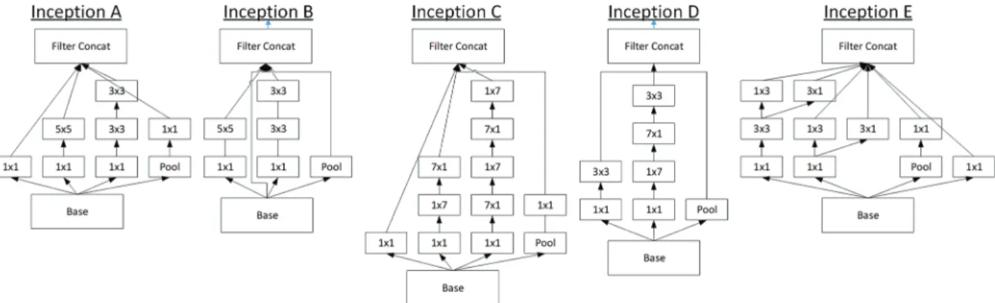
The Inception network is based on the concept that many activa-tions in deep convolution layers are either excessive (zero value) or redundant (highly correlated). Therefore, instead of going deeper in the CNN network, the balance between network width and depth should be maintained in order to provide optimal per-formance. The necessity of having efficient dimension reduc-tion leads to a sparse network with various filter sizes. As a result, the required computational reduction leads to bottleneck convolution [31] Szegedy, Vanhoucke [13] have suggested that replacingn×nconvolution by asymmetric convolutions with lower kernels and having generallyn× 1convolution after1 ×n convo-lution can significantly reduce computational costs. They have also noted that applying such factorization on early layers is not very effective. Therefore, to build Inception networks, we first used two simple primitive blocks (described in Section2.1.1) as the CNN base followed by one of the five asymmetric Inception blocks shown in Figure1.

2.1.3. The Resnet primitive blocks

The Resnet network was designed to address the challenge of over-coming the vanishing gradient problem in order to build deeper CNNs [11]. Instead of simply stacking layers, the middle layer learns the residual mapping of the input. This is done by adding a residual block as the identity connection from previous layers, thus allowing the residual mapping to be trained [11] as illustrated in Figure2.

2.2. Taguchi Method

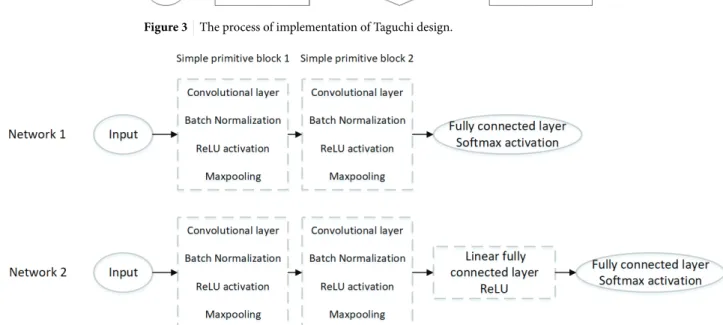
The Taguchi method is a statistically robust technique, proposed by Geninchi Taguchi [32], which fulfils two main roles, namely, find-ing factors that provide more variation in responses and findfind-ing the best levels of these factors that optimize CNN response. In the Taguchi method, initially a decision is made on which factors can be effective for the required response. Then, the levels of those factors are set. In Figure3, the Taguchi process block diagram is shown, where the initial process of finding the effective factors is depicted as the preparation block.

The next step in the Taguchi procedure is designing the experiment. This is based on the orthogonal matrix, determining in each run the levels of the control factors that must be taken. In statistical exper-imental design, orthogonality involves providing a matrix of runs that have statistically independent factors in their columns, where the levels in the columns of the independent factors are orthogonal to one another. Consequently, if the factor levels are considered as a vector, the inner product of mutual factor vectors in an orthogonal array must be zero [33].

Another property of the orthogonal matrix is that all the levels in each column must appear the same number of times. The above-mentioned two properties effectively reduce the number of exper-iments from full factorial design into a minimal number of runs, which still can provide enough knowledge in describing the effect of factors on the CNN performance. The minimum number of exper-iments needed to conduct the Taguchi method can be calculated based on the following equation:

N=

Number of variables

∑

i=1

(Levi–1)+ 1. (1)

whereNis the number of experiments andLeviis the number of

levels in theith factor.

The orthogonal matrices in a standard Taguchi design are pre-defined based on the number of controlling factors and levels. Consequently, the experiment is run according to the defined orthogonal array in order to determine and prepare the CNN responses for analysis. This step is shown as “design a new exper-iment” in Figure3. The relative percentage difference (RPD) in accuracy was used as the CNN response indicator that enables bet-ter understanding of the impact of the factors on the performance

(4)

Figure 2 Illustration of a residual block where the middle layer learns the residual mapping of the input, thus allowing the residual mapping to be trained [11].

of the CNN architecture. For the generated results, the RPD was calculated as follows:

RPD= xi–xmin xmin

× 100. (2)

wherexiis the responses obtained from theith run of the

experi-ment andxminis the minimum response obtained.

The results were analysed by comparing the mean controlling fac-tors and signal-to-noise ratios, as well as evaluating the analysis of variance (ANOVA), in order to investigate the significant factors. The preliminary design of the experiment was slightly changed after analysing the results mainly to determine the best controlling factor or the best levels of the controlling factors. After obtaining accept-able RPD results, the optimum level of each factor was implemented to obtain the best CNN according to defined objectives.

2.3. Design of Experiment

Before determining the factors and levels for designing the CNNs, a few preliminary designs were run to evaluate some hyperparam-eters. Two controlling factors, namely batch size with level values 8, 16, 32, and number of epochs with level values 5, 10, 20, were examined. It was found that neither the batch size nor the number of epochs affected the RPD accuracy. Their p-values in the ANOVA were 0.23 and 0.71, respectively. However, it was necessary to define their values in the network. As the larger batch size resulted in faster training and less over fitting, the selected batch size value was 32. Smaller values for the number of epochs typically led to faster running of the whole procedure of learning. Therefore, the chosen number of epochs was 5.

The following hyperparameters were selected as the factors in our search space: learning rate, augmentation types, number of filters, and size of kernel.

Learning rate:In order to have fast network convergence during

training, the optimum selection of the learning rate was essential.

When the chosen learning rate was too small, training took too long to converge or the optimizer became trapped in local minima, hence the loss function could not be updated to generalize the net-work. When the chosen learning rate was too large, the network did not always converge as it might have overpassed the minimum loss function, and hence, made the loss function worse.

Augmentation:Large data in deep learning normally yields better

performance; however, it is not always possible to have large data. As neural networks have invariance characteristics, data augmen-tation can generate more data without the need for additional data collection. In order to select the type of data augmentation, it is nec-essary to consider the nature of the data. In the proposed study, the implemented data was linear spectrum reflectance. Accord-ing to the nature of the data, flippAccord-ing (horizontal and vertical) and normalization were the most suitable transformations for data augmentation.

Number of filters and kernel sizes:In the first two layers of the

first design, two simple primitive blocks were used. In the first layer, lower levels for the number of filters were used (4, 8, 16, 32), since the network typically extracts basic features in this layer. The larger levels for the number of filters were selected in the second layer (32, 64, 128, 256), because this layer combines the basic features and produces more complex features for classification. The next factors investigated in the proposed study were the kernel sizes. The levels of 3 and 5 were selected for the investigation.

Four experiments were designed, based on (i) simplified primitive cells, (ii) modified Inception cells, (iii) modified Resnet cells, and (iv) an experiment comparing the performances of all three prim-itive cells. The pytorch deep learning library [34] was used for all trainings. GeForce GTX 1080Ti Nvidia GPU was the hardware plat-form for data processing, which has a 11 GB memory, a 352-bit interface used in conjunction with an IntelⓇCoreTM _i7-7800X

X-series Processor.

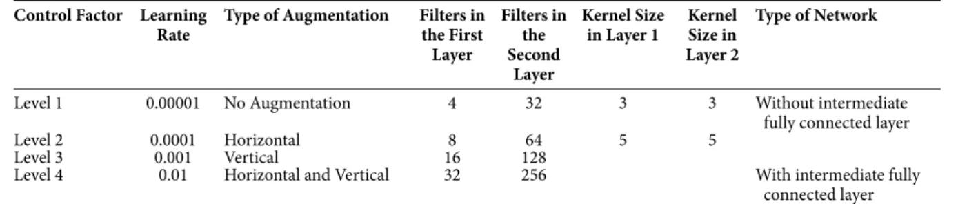
2.3.1. First design of experiment

Two simple structures were suggested for the first design, as shown in Figure4. The first structure had one fully connected classification output layer with soft max activation. The second structure had an extra fully connected layer with a ReLu activation.

The effect plot and accuracyversusthe size of the middle connected layer, which are the results of the preliminary experiment that was designed to choose the number of nodes in the extra fully connected layer, are shown in Figure5.

According to the Bonferroni post-hoc test, which measures the sig-nificance of the pairwise differences between factor levels, there was no significant difference between the levels with values of 32, 64, 128, and 256 (Table1). Therefore the 128 value was selected based on the best signal-to-noise-ratio performance. With this result, the first DOE was designed as illustrated in Table2.

2.3.2. Second design of experiment

The next DOEs were designed to examine the effect of using vari-ous Inception networks. The same controlling factors were selected for the Inception networks, however, they were chosen in three

(5)

Figure 3 The process of implementation of Taguchi design.

Figure 4 Two different convolutional neural networks (CNN) structures comprising simple primitive blocks.

Figure 5 Preliminary experiment results for determining the value of middle fully connected layer in the first design. A) Effect and B) accuracyversusthe size of the middle connected layer.

Table 1 Analysis of variance for comparing the different number of nodes in the middle fully connected layer, the response was the relative percentage difference in accuracy.

Df Sum Sq Mean Sq F value Pr(>F)

Fully connected size 1 2388.6 2388.6 10.803 0.001457** Residuals 88 19457.7 221.11

Signif. codes: 0 ‘***’ 0.001 ‘**’ 0.01 ‘*’ 0.05 ‘.’ 0.1 ‘ ’ 1.

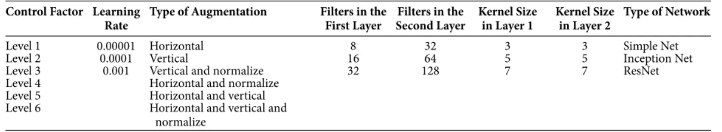
levels, except the type of network, which was selected according to the various Inception design. These levels are shown in Table3. 2.3.3. Third design of experiment

Another design introduced here, was based on the Resnet net-work. This included two simple primitive blocks following two primitive residual layers. Each residual layer can downsample from

its previous layer and produce the required number of residual blocks. The learning rate was used in exactly the same way as the previous design, where there were two residual layers. In each resid-ual layer, the number of blocks and the number of filters in each block and its kernel size were investigated to determine how effec-tive they are and what are their optimum values for the current network and dataset. Various types of augmentation were also investigated, namely horizontal, vertical, and vertical and normal-ized augmentation, as illustrated in Table4.

2.3.4. Fourth design of experiment

The last DOE was designed to compare the simple network, the Inception network, and Resnet. According to our previous investigation, the most effective levels for the learning rate were

(6)

Table 2 The design of experiment for the simple convolution network.

Control Factor Learning Rate

Type of Augmentation Filters in the First Layer Filters in the Second Layer Kernel Size in Layer 1 Kernel Size in Layer 2 Type of Network

Level 1 0.00001 No Augmentation 4 32 3 3 Without intermediate fully connected layer Level 2 0.0001 Horizontal 8 64 5 5

Level 3 0.001 Vertical 16 128

Level 4 0.01 Horizontal and Vertical 32 256 With intermediate fully connected layer

Table 3 The design of experiment for the Inception convolution networks.

Control Factor Learning Rate

Type of Augmentation Filters in the First Layer Filters in the Second Layer Kernel Size in Layer 1 Kernel Size in Layer 2 Type of Network

Level 1 0.00001 Horizontal and vertical 4 32 3 3 Inception A Level 2 0.0001 Vertical 8 64 5 5 Inception B Level 3 0.001 Vertical and normalize 16 128 7 7 Inception C

Level 4 Inception D

Level 5 Inception E

Table 4 The design of experiment for the residual convolution network.

Resnet Blocks Used in Both Resnet Layers

Type of Augmentation Filters in the First Resnet Layer Filters in the Second Resnet Layer Kernel Size in Layer 1 Kernel Size in Layer 2 Level 1 0.00001 1 Horizontal 8 32 3 3 Level 2 0.0001 2 Vertical 16 64 5 5

Level 3 0.001 3 Horizontal and vertical 32 128 7 7

Level 4 4

Level 5 5

Level 6 6

chosen to be (0.01, 0.001, 0.0001). Additionally, the appropriate number of filters in each layer and kernel sizes were selected accord-ingly. All types of augmentation introduced in the previous designs were researched in this design as well. All the factors that lead to the design are shown in Table5.

According to the number of factors and levels, the orthogonal array L16 was chosen for the first Design since it has four factors with four levels, and three factors with two levels. The orthogonal array L18 was chosen for the following designs because it has six factors with one three levels and one factor with six levels. In order to signifi-cantly reduce the possibility of random results, all the designs were run with five replications. The replication was produced by using a random seed to ensure the same results are produced in future runs. All the DOEs and results were designed and analysed in Software R, Version 3.5.1 (2018-07-02).

3. RESULTS AND DISCUSSIONS

3.1. Evaluation Metrics

Since for an orthogonal array the design is balanced, the factor lev-els are weighed equally, making the effects of factors independent from one another. Therefore, each factor can be assessed indepen-dently, hence reducing the time and cost of the experiment. This characteristic helps to easily compare the mean of each level in a

particular factor to determine how effective each level is in chang-ing the response. This characteristic can typically be displayed through the mean in the effect plot. Similarly, the signal-to-noise ratio is another metric that can evaluate the factor levels. In the current study, the aim was not to only determine which factor lev-els were effective in producing better accuracy, but also to ensure stable factor levels in order to generalize these factors for future classification problems. Therefore, the nominal-the-best approach was chosen to measure the signal-to-noise ratio as it evaluates the levels around the mean and considers changing other factors according to the orthogonal array. The signal-to-noise ratio can be calculated as follows:

If we consider the data to bey1,y2, … ,ynthen:

S

N= 10 ∗log y2

s2, (3)

whereyandsare the average and standard deviation of the data, respectively.

Finally, ANOVA was used to analyse the results. Since the aim of the proposed study was to reduce the computational cost while improv-ing the accuracy, if a factor was significantly important, the level that produced the best accuracy was selected. Similarly, if the factor was not statistically significant, the optimum level of the factor was selected from the effect plots in order to reduce the computational cost.

(7)

Table 5 Design of experiment for comparison of Resnet, Inception, and simple network.

Type of Augmentation Filters in the First Layer Filters in the Second Layer Kernel Size in Layer 1 Kernel Size in Layer 2 Type of Network

Level 1 0.00001 Horizontal 8 32 3 3 Simple Net Level 2 0.0001 Vertical 16 64 5 5 Inception Net Level 3 0.001 Vertical and normalize 32 128 7 7 ResNet Level 4 Horizontal and normalize

Level 5 Horizontal and vertical Level 6 Horizontal and vertical and

normalize

3.2. Designs Evaluation

3.2.1. Design 1

Figure6shows the effect plots of mean and signal-to-noise ratio of controlling variables introduced in the first design (DOE for the simple CNN). The first controlling factor was the learning rate. Since the aim of learning rate is to control and adjust the network weights to reduce network loss, having appropriate initial learning rate helps the network to converge faster, hence reducing the com-putation time. According to the ANOVA, the effect of the learning rate was significant. Similarly, the effect plots demonstrated that the best level of learning rate was 0.0001. For the rest of the DOEs, the best obtained leaning rate was still 0.0001.

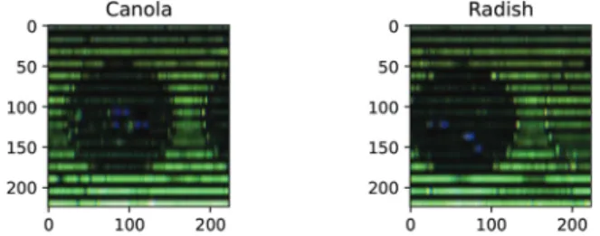
The next factor investigated was the augmentation type. In the first design, four types of augmentation were selected; vertical, horizon-tal, vertical and horizonhorizon-tal, and no augmentation. These augmen-tations were chosen according to the nature of the data. The data applied in the current study were three spectral laser reflectance values (at three different wavelengths) collected by the plant discrimination unit (PDU), PDU collects linearly three laser reflectance values [35]. Accumulation of these linear responses resulted in three layers of two-dimensional inputs. Wild leaf plants (Canola and Radish) were considered as two input classes. Two hundred plants were grown. 2400 spectral data were collected for each plant stage. Data were collected in five different stages, three days after early germination for five consecutive weeks. A total of 12000 data were generated for each class. Sixty percent of the data set was kept for training and the rest was equally divided for val-idation and testing. Training, valval-idation, and testing plants were kept strictly separated to ensure the generalization of the study. A sample data set used for training is shown in Figure7. Vertical augmentation changed the order of the laser beams from end to beginning. The horizontal augmentation changed the direction of 2D arrays of data. The results show that the combination of hor-izontal and vertical augmentation significantly changed the value RPD accuracy.

The role of filters in the first layer was to help learning the basic features and in the following layer and combine these features to produce deep learning according to more complex features. When there were not much basic features in the data, the number of filters in the first layer could be reduced to minimize the computational cost. Results showed that with 16 or 32 filters in the first layer and 128 or 256 filters in the second layer, better RPD accuracy could be obtained. While the difference between the number of filters in the first layer and second layer were not statistically significant, the interaction between the filters in these two layers provided signifi-cant differences in RPD accuracy.

The next two controlling factors introduced were the kernel sizes. According to effect plots, there was slight improvement using5 × 5 kernel rather than3 × 3kernel, due to nature of the data. As can be seen from Figure7, there is gap between laser reflectance responses. This is because at the end of each block there was a max pooling layer which returned the maximum of a2 × 2kernel, where this gap did not provide much information for the network. Therefore,5 × 5 kernels were able to provide slightly better accuracy than the3 × 3 kernels, however, this difference was not significant.

In the last controlling factor, the two simple CNNs shown in Figure4were compared. One CNN was with two simple blocks and a fully connected layer for classification, while the other CNN with an extra middle fully connected layer, to be able to combine all the extracted feature for classification following ReLu function. The results show that there was no significant difference between these factors, with the CNN without the middle fully connected layer pro-viding better RPD accuracy. This is due to the low number of fea-tures in our selected dataset, meaning that when a dataset is simpler according to its number of features, there is no need to make the network more complex and increase the computational expenses. 3.2.2. Design 2

Figure8shows effect plots of the means and signal-to-noise ratios for the factors of the second design. As can be seen from Figure8, the 0.0001 value was still the best for initialization of learning rate. In this design, three types of augmentation were investigated, namely vertical, vertical and normalized, and horizontal and verti-cal augmentation. Figure8clearly shows that using horizontal and vertical augmentation still provided significantly better RPD accu-racy in terms of both mean plot and signal-to-noise ratio.

Note that while only the number of filters used in the first layer significantly changed the RPD accuracy, the results show that the interaction of the number of filters used in the first layer and the number of filters used in the second were significantly important in the second design based on the use of Inception primitive blocks. This shows that in the second DOE, the combination of features made the second layer more effective in achieving higher accu-racy. The optimum number of filters in the first and second layers according to effect plot were 16 and 64, respectively.

According to the mean of effect plots, the best kernel size was5 × 5. The kernel size in the first layer significantly changed the value of RPD accuracy, while in the second layer, the change was not statis-tically significant. This is attributed to the asymmetry property of the Inception blocks used after the second layer, which automati-cally combines the various kernels and does not need to particularly fix their size in the second layer.

(8)

Figure 6 Effect plots of mean and signal-to-noise ratio for seven controlling factors of the simple convolutional neural network (CNN) used in the first design. Each plot is for one of the controlling factors, namely: A) Learning rate, B) Type of augmentation, C) Number of filters in the first simple primitive block, D) Number of filters in the second simple primitive block, E) Convolution kernel size in the first block, F) Convolution kernel size in the second block, G) Type of network (Net1 represent the simple CNN without middle fully connected layer and Net2 represent simple CNN with middle fully connected layer).

(9)

Figure 7 A sample data used as combination of three-layer laser spectral reflectance.

The best RPD accuracy was obtained by the network that used the Inception B block (shown in Table1), which had the simplest Inception block structure with minimum combination of 3 × 3 kernels. High accuracy was attained in this case because replac-ing 5 × 5 convolution by asymmetric convolutions with lower kernels and having3 × 1convolution after3 × 3convolution signifi-cantly reduced the computational costs. Similarly, the worst results occurred in CNN with Inception C block, which went deeper in the network (up to five layers after the base layer) and used more com-plex combinations of kernels with1 × 7sizes and7 × 1sizes. This result could be because applying more complex kernel sizes such as 1 × 7and7 × 1to extract more complex features were not appar-ently suitable for the dataset used in the proposed research.

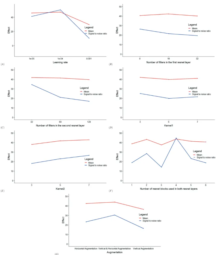
3.2.3. Design 3

Figure9shows effect plots of the means and signal-to-noise ratios for the factors of the third design. Consistent with previous results, the best learning rate in the third designed network was 0.0001. The augmentation types selected were horizontal, vertical, and horizon-tal and vertical augmentation. The combination of horizonhorizon-tal and vertical augmentation provided significantly better RPD accuracy since it provided more scenarios for the network learning process. In each residual layer, the effects of using various numbers of resid-ual blocks were investigated to determine the importance of going deeper for classification. The results showed that the best mean RPD accuracy was obtained by using four blocks, while the differ-ence of using various blocks were not statistically significant. The other insignificant parameters here were the number of filters and kernel sizes. As can be seen from Figure9, the difference between the means of RPD accuracy was insignificant. This is because when the residual layer can learn from the previous layer and possesses a low number of features, it does not required more filters. Instead, one can go deeper and use the residual layers, which make the effect of number of filters and kernel sizes less important for a dataset of low features. Therefore, in this case, the minimum level of filters can be selected to reduce the computational cost.

3.2.4. Design 4

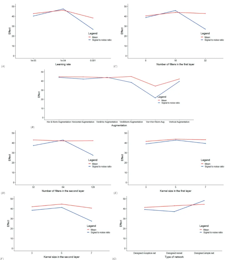
Figure10shows effect plots of the means and signal-to-noise ratios for the factors of the comparison design. In the last DOE, three designed CNNs were compared. The best learning rate obtained was 0.0001, which was in accordance with the previous results. The variations between using various augmentations were slight, while the vertical and horizontal augmentation resulted in an acceptable

signal-to-noise ratio and a mean effect plot. According to the effect plots, a suitable number of filter size can be chosen, 16 for the first layer and 64 for the second layer. While the impact of each filter was not statistically significant, the interaction between them showed that in order to have proper feature extraction, the interac-tion between filters is important. Based on the effect plots, the opti-mum kernel sizes was5 × 5kernel, which was the result of the type of the used data. In comparing the three CNNs, the simple designed CNN showed significantly better effect plot of RPD accuracy and lower computational cost since the number of parameters in this CNN is lower than those in the other CNNs.

3.3. Comparison of CNNs with and without

Optimizations

The aim of the last investigation was to introduce an approach that determines the simplest network that could be classified as efficient as the manually-engineered network. The previously-discussed agricultural dataset was also chosen to evaluate the optimization procedure. The designed CNNs were compared based on their test-ing accuracies before and after parameter optimization. In order to have better comparison, the network was activated with five vari-ous seeds, namely cuda and pytorch random seeds. Figure11shows the average testing accuracies of the investigated CNNs activated with five different random seeds. The comparison results show that, for all the cases, there were improvements in the testing accuracy. Generally, there was a correlation between the number of significant controlling factors in the optimization process and the amount of improvement in accuracy. The Inception network had five significant controlling factors, resulting in the highest improve-ment in accuracy, while the Resnet network had only three sig-nificant factors, displaying the lowest improvement in accuracy Tables6–9.

4. CONCLUSION

In this paper, four main DOE have been proposed and investi-gated to determine and optimize the significant factors that affect the performance of three simplified CNN architectures, namely, the VGG network, the Inception network, and the Resnet network. DOE algorithms based on utilizing Taguchi statistical methods have been developed for optimizing CNN parameters, and then tested using spectral agricultural data. Results have shown that, for all investigated CNN architectures, there was measurable improve-ment in accuracy in comparison with un-optimized CNNs, and

(10)

Figure 8 The effect plot of mean and signal-to-noise ratio for the second design. The effect plot of seven variable investigated in here. A) Learning rate, B) Type of augmentation, C) Number of filters used in the first layer, D) Number of filters use in the second layer, E)

(11)

Figure 9 The effect plot of mean and signal-to-noise ratio for the third design. The variable investigated were A) Learning rate, B) Number of blocks used in the Resnet layers, C) Type of augmentation, D) Number of filters used in the first Resnet layer, E) Number of filters used in the second Resnet layer, F) Convolution kernel size in the first Resnet layer, G) Convolution kernel size in the second Resnet layer.

(12)

Figure 10 The effect plots of mean and signal-to-noise ratio of the fourth design for comparison of designed simple convolutional neural network (CNN), designed Inception net, and designed Resnet. Each plot belong to one of the controlling variable namely: A) Learning rate, B) Type of augmentation, C) Number of filters in the first primitive block, D) Number of filters in the second primitive block, E) Convolution kernel size in the first block, F) Convolution kernel size in the second block, G) Type of network (designed Inception, designed Resnet, designed simple net).

(13)

Figure 11 Average testing accuracies of the convolutional neural networks (CNNs) activated with five different random seed.

Table 6 Analysis of variance for comparing factors according to the first DOE, the response was the relative percentage difference in accuracy.

Learning rate 1 21387.0 21387.0 240.3860 < 2.2e–16*** Augmentation 1 1201.2 400.4 4.5005 0.006079 ** Number of filters in the first block 1 524.0 524.0 5.8902 0.017841 * Number of filters in the second block 1 33.1 33.1 0.3722 0.543827 Kernel size in block 1 1 8.0 8.0 0.0895 0.765775 Kernel size in block 2 1 100.4 100.4 1.1282 0.291857

Type of network 1 2.3 2.3 0.0264 0.871462

Interaction between filters 1 556.4 556.4 6.2541 0.014769 *

Residuals 69 6138.9 88.96

DOE = design of experiment; Signif. codes; 0 ‘***’ 0.001 ‘**’ 0.01 ‘*’ 0.05 ‘.’ 0.1 ‘ ’ 1.

Table 7 Analysis of variance for comparing factors according to the second DOE, the response was the relative percentage difference in accuracy.

Learning rate 1 24.53 24.53 1.5470 0.217459 Augmentation 2 123.43 61.71 3.8914 0.024664 * Number of filters in the first block 1 175.63 175.63 11.0742 0.001358 ** Number of filters in the second block 1 14.73 14.73 0.9290 0.338209 Kernel size in block 1 1 71.95 71.95 4.5366 0.036458 * Kernel size in block 2 1 6.71 6.71 0.4231 0.5173687 Type of network 1 221.46 44.29 2.7928 0.022859 * Interaction between filters 1 120.34 120.34 7.5881 0.007369 **

Residuals 75 1189.45 15.86

DOE = design of experiment; Signif. codes: 0 ‘***’ 0.001 ‘**’ 0.01 ‘*’ 0.05 ‘.’ 0.1 ‘ ’ 1.

Table 8 Analysis of variance for comparing factors according to the third DOE, the relative percentage difference in accuracy was considered as response.

Learning rate 1 5655.7 5655.7 50.4665 4.245e-10 *** Augmentation 2 974.0 487.0 4.3456 0.01612 * Number of filters in the first block 1 12.0 12.0 0.1067 0.74481 Number of filters in the second block 1 72.9 72.9 0.6504 0.42232 Kernel size in block 1 1 22.2 22.2 0.1978 0.65772 Kernel size in block 2 1 361.8 361.8 3.2281 0.07611

Resnet blocks 1 20.0 20.0 0.1783 0.67392

Residuals 81 9077.5 112.1

that the Inception network yields the highest improvement (∼6%) in accuracy compared to simple CNN (∼5%) and Resnet CNN counterparts (∼ 2%). Generally, based on the proposed Taguchi

experimental designs, the optimum hyperparameter of a CNN can be determined in order to provide a simpler and faster trainable net-work with performance improvements.

(14)

Table 9 Analysis of variance for comparing factors according to the fourth DOE, the relative percentage difference in accuracy was considered as response.

Learning rate 1 689.74 689.74 22.4571 9.973e-06 *** Augmentation 5 1234.51 246.90 8.0388 4.122e-06 *** Number of filters in the first block 1 57.39 57.39 1.8685 0.175736 Number of filters in the second block 1 3.45 3.45 0.1123 0.738422 Kernel size in block 1 1 43.93 43.93 1.4304 0.234546 Kernel size in block 2 1 30.04 30.04 0.9780 0.325866 Type of network 2 439.45 219.72 7.1539 0.001434 ** Interaction between filters 1 250.80 250.80 8.1659 0.005522 **

Residuals 75 2303.52 30.71

CONFLICT OF INTEREST

Authors have no conflict of interest to declare.

ACKNOWLEDGMENTS

The research is supported by Edith Cowan University, the Grains Research and Development Corporation (GRDC), Australian Research Council, Photonic Detection Systems Pty. Ltd, Australia, and Pawsey Supercomput-ing Centre.

REFERENCES

[1] A. Krizhevsky, I. Sutskever, G.E. Hinton, Imagenet classification with deep convolutional neural networks, Commun. ACM. 60 (2017), 84–90.

[2] W. Hu,et al., Deep convolutional neural networks for hyperspec-tral image classification, J. Sens. 2015 (2015), 1–12.

[3] A. Karpathy,et al., Large-scale video classification with convolu-tional neural networks, in Proceedings of the IEEE conference on Computer Vision and Pattern Recognition, Columbus, 2014. [4] Y. Wang,et al., Low power convolutional neural networks on a

chip, in 2016 IEEE International Symposium on Circuits and Sys-tems (ISCAS), IEEE, Montreal, 2016.

[5] C. Zhang,et al., Optimizing fpga-based accelerator design for deep convolutional neural networks, in Proceedings of the 2015 ACM/SIGDA International Symposium on Field-Programmable Gate Arrays, ACM, Monterey, 2015.

[6] J. Jin, et al., An efficient implementation of deep convolu-tional neural networks on a mobile coprocessor, in 2014 IEEE 57th International Midwest Symposium on Circuits and Systems (MWSCAS), IEEE, Austin, 2014.

[7] V. Sze, et al., Hardware for machine learning: challenges and opportunities, in 2017 IEEE Custom Integrated Circuits Confer-ence (CICC), IEEE, Austin, 2017.

[8] F.N. Iandola, et al., Squeezenet: alexnet-level accuracy with 50x fewer parameters and <0.5 mb model size, arXiv preprint arXiv:1602.07360, 2016.

[9] A. Krizhevsky, One weird trick for parallelizing convolutional neural networks, arXiv preprint arXiv:1404.5997, 2014.

[10] K. Simonyan, A. Zisserman, Very deep convolutional networks for large-scale image recognition, arXiv preprint arXiv:1409.1556, 2014.

[11] K. He,et al., Deep residual learning for image recognition, in Pro-ceedings of the IEEE Conference on Computer Vision and Pattern Recognition, Honolulu, 2016.

[12] G. Huang,et al., Densely connected convolutional networks, in Proceedings of the IEEE Conference on Computer Vision and Pattern Recognition, Honolulu, 2017.

[13] C. Szegedy,et al., Rethinking the inception architecture for com-puter vision. in Proceedings of the IEEE Conference on Comcom-puter Vision and Pattern Recognition, Las Vegas, 2016.

[14] B. Baker,et al., Designing neural network architectures using rein-forcement learning, arXiv preprint arXiv:1611.02167, 2016. [15] E. Real,et al., Large-scale evolution of image classifiers, arXiv

preprint arXiv:1703.01041, 2017.

[16] P. Verbancsics, J. Harguess, Generative neuroevolution for deep learning, arXiv preprint arXiv:1312.5355, 2013.

[17] P. Verbancsics, J. Harguess, Image classification using genera-tive neuro evolution for deep learning, in 2015 IEEE Winter Conference on Applications of Computer Vision (WACV),IEEE, Waikoloa, 2015.

[18] B. Zoph, Q.V. Le, Neural architecture search with reinforcement learning, arXiv preprint arXiv:1611.01578, 2016.

[19] R. Goebel,et al., Explainable AI: the new 42?, in: A. Holzinger, P. Kieseberg, A. Tjoa, E. Weippl (Eds.), International Cross-Domain Conference for Machine Learning and Knowledge Extraction, Springer, Cham, 2018.

[20] A. Holzinger,et al., What do we need to build explainable AI sys-tems for the medical domain?, arXiv preprint arXiv:1712.09923, 2017.

[21] M. Mamourian,et al., Optimization of mixed convection heat transfer with entropy generation in a wavy surface square lid-driven cavity by means of Taguchi approach, Int. J. Heat Mass Transfer. 102 (2016), 544–554.

[22] M.K. Balki, C. Sayin, M. Sarikaya, Optimization of the operating parameters based on Taguchi method in an SI engine used pure gasoline, ethanol and methanol, Fuel. 180 (2016), 630–637. [23] W.C. Chen,et al., Optimization of the plastic injection molding

process using the Taguchi method, RSM, and hybrid GA-PSO, Int. J. Adv. Manuf. Technol. 83 (2016), 1873–1886.

[24] A. Tsiolikas,et al., Optimization of neural network parameters using Taguchi robust design: application in plasma arc cutting process, in 2017 Fourth International Conference on Mathematics and Computers in Sciences and in Industry (MCSI), Corfu, 2017. [25] M. Peker, A new approach for automatic sleep scoring:

combin-ing Taguchi based complex-valued neural network and complex wavelet transform, Comput. Methods Prog. Biomed. 129 (2016), 203–216.

[26] T.M. Patel, N.M.J.A.I. Bhatt, Optimizing neural network parame-ters using Taguchi’s design of experiments approach: an applica-tion for equivalent stress predicapplica-tion model of automobile chassis, Auto. Innov. 1 (2018), 381–389.

(15)

[27] G.J.Q.R. Taguchi, Taguchi Techniques for Quality Engineering, McGraw-Hill, New York, 1987.

[28] V. Nair, G.E. Hinton, Rectified linear units improve restricted boltzmann machines, in Proceedings of the 27th International Conference on Machine Learning (ICML-10), Haifa, 2010. [29] S. Ioffe, C.J.a.p.a. Szegedy, Batch normalization: accelerating deep

network training by reducing internal covariate shift, in Proceed-ings of the 32nd International Conference on Machine Learning, Lille, 2015.

[30] J.T. Springenberg,et al., Striving for simplicity: the all convolu-tional net, arXiv preprint arXiv:1412.6806, 2014.

[31] H. Lee, et al., Convolutional deep belief networks for scal-able unsupervised learning of hierarchical representations, in

Proceedings of the 26th Annual International Conference on Machine Learning, ACM, Montreal, 2009.

[32] C. Szegedy,et al., Going deeper with convolutions, in Proceedings of the IEEE Conference on Computer Vision and Pattern Recog-nition, Boston, 2015.

[33] U. Grömping, H. Xu, Generalized resolution for orthogonal arrays, Annu. Stat. 42 (2014), 918–939.

[34] A. Paszke,et al., Automatic differentiation in PyTorch, in NIPS 2017 Workshop Autodiff Homepage, 2017.

[35] S. Akbarzadeh, et al., Plant discrimination by support vector machine classifier based on spectral reflectance, Comput. Elec-tron. Agric. 148 (2018), 250–258.