Efficient Vector Quantization for Fast Approximate Nearest Neighbor Search

(1)

ANTON MURAVEV

EFFICIENT VECTOR QUANTIZATION FOR FAST APPROXIMATE

NEAREST NEIGHBOR SEARCH

Master of Science thesis

Examiners:

Prof. Moncef Gabbouj Dr. Alexandros Iosifidis

Examiner and topic approved in the Faculty Council meeting of

Computing and Electrical Engineering Faculty on 4th May 2016

(2)

ABSTRACT

ANTON MURAVEV: Efficient Vector Quantization for Fast Approximate Nearest Neighbor Search

Tampere University of Technology

Master of Science Thesis, 49 pages, 0 Appendix pages June 2016

Master’s Degree Programme in Information Technology Major: Data Engineering

Examiners: Prof. Moncef Gabbouj, Dr. Alexandros Iosifidis

Keywords: approximate nearest neighbor search, product quantization, additive quantization

Increasing sizes of databases and data stores mean that the traditional tasks, such as lo-cating a nearest neighbor for a given data point, become too complex for classical solu-tions to handle. Exact solusolu-tions have been shown to scale poorly with dimensionality of the data. Approximate nearest neighbor search (ANN) is a practical compromise be-tween accuracy and performance; it is widely applicable and is a subject of much re-search.

Amongst a number of ANN approaches suggested in the recent years, the ones based on vector quantization stand out, achieving state-of-the-art results. Product quantization (PQ) decomposes vectors into subspaces for separate processing, allowing for fast lookup-based distance calculations. Additive quantization (AQ) drops most of PQ con-straints, currently providing the best search accuracy on image descriptor datasets, but at a higher computational cost. This thesis work aims to reduce the complexity of AQ by changing a single most expensive step in the process – that of vector encoding. Both the outstanding search performance and high costs of AQ come from its generality, there-fore by imposing some novel external constraints it is possible to achieve a better com-promise: reduce complexity while retaining the accuracy advantage over other ANN methods.

We propose a new encoding method for AQ – pyramid encoding. It requires significant-ly less calculations compared to the original “beam search” encoding, at the cost of an increased greediness of the optimization procedure. As its performance depends heavily on the initialization, the problem of choosing a starting point is also discussed. The re-sults achieved by applying the proposed method are compared with the current state-of-the-art on two widely used benchmark datasets – GIST1M and SIFT1M, both generated from a real-world image data and therefore closely modeling practical applications. AQ with pyramid encoding, in addition to its computational benefits, is shown to achieve similar or better search performance than competing methods. However, its current ad-vantages seem to be limited to data of a certain internal structure. Further analysis of this drawback provides us with the directions of possible future work.

(3)

The work presented in this thesis was carried out at the Department of Signal Pro-cessing, Tampere University of Technology (TUT) over a period of 7 months – from October 2015 till May 2016. Throughout this period the author was employed as a re-search assistant in the MUVIS group.

I would like to express my utmost gratitude to professor Moncef Gabbouj for an oppor-tunity to work as a part of the group and for his invaluable advice, which will undenia-bly prove useful in my future scientific career. I am very grateful to my supervisor Mr. Ezgi Can Ozan for providing such an interesting topic to work with and for fruitful discussions, which motivated many positive changes in the proposed methods. I would also like to thank Dr. Alexandros Iosifidis for his guidance and important feedback throughout the work.

Finally, I offer my sincere gratitude to my parents. Despite the great distance between us, their support and encouragement were immense throughout the whole period of my studies, including the thesis preparation.

Tampere, June 2016

(4)

1. INTRODUCTION

The nearest neighbor (NN) search, or the problem of matching the given object to the most similar one from the given group, is extremely common; it is not only specific to science or engineering, but permeates the everyday life in many forms, such as recogni-tion. Its technical definition can vary based on the nature of the objects and how their similarity is established. The latter is usually defined as a function, providing a numeric output value. The objects of search are commonly vectors, allowing for a variety of sim-ilarity measures to be used, both metric and nonmetric.

While the search problem is trivial when the number of objects to consider is small, the advances in computer science and technology lead to a consistent growth of data sizes. For this reason the data structures allowing efficient search were extensively studied since 1970s [1]. Branch-and-bound approach in particular resulted in numerous types of search trees, allowing for queries to be of logarithmic complexity with respect to data size [2]. Space partitioning would remain dominant for decades thereafter.

The emergence of Big Data has led to reconsideration of many previously established solutions [3][4]. This new environment presents a number of challenges, one of which is the sheer volume of the databases. Traditional algorithms and methods commonly be-come computationally infeasible in such scenarios, sometimes to the point of complete inapplicability. The nearest neighbor search techniques were no exception from this; many well-established data structures were found to lose their advantages completely in higher-dimensional spaces, becoming inferior to exhaustive calculations [5].

Many current practical applications involving the search do not require perfectly accu-rate results. For instance, when information retrieval is performed, the returned docu-ments or images are often deemed acceptable if they are relevant; the exact definition of relevance varies on case by case basis, but can generally be taken to mean “similar enough to the perfect outcome”. This factor, combined with previously mentioned com-putational costs issue, leads to the notion of the approximate nearest neighbor (ANN) search, which has been the focus of much recent research.

The focus of approximate search techniques is as much on accuracy as it is on scalabil-ity and low costs, both in computation and in memory use. Removing the requirement for an exact solution allows for a considerable complexity reduction, making the ap-proximate search preferable in many practical scenarios. Some of the current large-scale applications include:

(7)

 large-scale cluster analysis, as many common algorithms (e.g. k-means, hierar-chical clustering) require NN search as an intermediate step [8];

 computer vision [9];

 recommendation systems [10];

 pattern recognition and classification [11][12][13].

Locality sensitive hashing (LSH) introduced a breakthrough in ANN search algorithms, leading to an emergence of the large family of hashing-based techniques [14]. All of these produce binary codes from the data, and Hamming distance between the codes is used as a substitute for the original similarity measure. The hash function is required to produce similar codes for similar data inputs, and vice versa. The exact choice of the hashing function naturally depends on the similarity measure used. Later algorithms attempted to learn suitable hash functions from the data itself, instead of just using the static formulations. Due to extensive research the properties of LSH and its derivatives are relatively well-understood. There is a wide variety of hash functions for many simi-larity measures and use cases. Due to these factors and typically modest computational costs, hashing-based techniques have been widely applied in practice and still draw the academic attention [7][14][15].

The drawback of this family of methods is the relatively poor search accuracy. In addi-tion to the imperfecaddi-tion of the hash funcaddi-tions and the locality criterion, the binary codes simply lack the representation power to preserve the original pairwise distances. While reducing (compressing) the data does provide the approximate search benefits, it could be more efficient, if the same similarity measure could be retained after the transfor-mation. Under the assumption of Euclidean distance (which often holds in practice) the data can be compressed (quantized) with an algorithm known as vector quantization (VQ), which operates completely in the original space [16].

While ANN search can be performed with VQ, it is not a practical solution. VQ is sus-ceptible to a “curse of dimensionality”, leading to exponential growth in calculations and memory requirements as the data grows in dimensions [17]. However, other tech-niques that avoid the issue have been derived in recent years, resulting in a quantization-based methods forming a family of their own [18]. These methods often enjoy a strong advantage over state-of-the-art hashing-based ANN solutions [18][19][20].

One example of such is additive quantization (AQ) [21]. It represents the original vec-tors as sums of vecvec-tors chosen from a limited set, the contents of which are learned from the data. AQ has been shown to achieve state-of-the-art search performance, but at the cost of computational complexity, which limits its applicability in practice.

Finding an accurate AQ representation for any given vector is called encoding and is known to be NP-hard, leading to the adoption of various heuristics, but even then it

(8)

con-stitutes the majority of AQ computational costs. Any vector to be added to the database needs to be encoded; the learning of AQ also requires numerous runs of encoding. De-veloping encoding algorithms that achieve the balance between complexity and accura-cy is thus of major importance, as outlined by the AQ authors [21].

Several variants of AQ formulation have been proposed since, each taking a different approach to simplification of the encoding problem [22][23]. These approaches take form of additional constraints, resulting in some generality loss. As the representation becomes more limited, the search performance is decreased. However, the computation-al gains from the simpler encoding result in more practiccomputation-al solutions.

This thesis work aims to provide a novel encoding algorithm that does not rely on ex-plicit constraints. Employing a previously unused heuristic, the goal is to achieve the compromise between the complexity and quality of encoding.

1.1 Thesis outline

The structure of the remainder of the thesis is described below.

Chapter 2 provides the problem formulations for both exact and approximate nearest neighbor search. Rough outline of the most common exact solutions follows. Finally, a very large family of hashing-based methods for approximate is presented. These ap-proaches have been extensively researched, received a wide variety of practical applica-tions and remained dominant in performance until the emergence of vector quantization family.

Chapter 3 presents the approximate search schemes based on vector quantization. Basic concepts common to many methods are presented first, followed by detailed descrip-tions of two most influential soludescrip-tions – product quantization (PQ) and additive quanti-zation (AQ). Several derivative methods are also briefly covered. Complexity and memory requirement estimates are provided for all the operations (if possible).

Chapter 4 explores the proposed encoding methods – pyramid encoding and residual pyramid encoding – from motivation to application and related costs. The influence and choice of initialization is discussed.

Chapter 5 covers the experimental evaluation of the proposed methods against the ref-erence results of other recent approaches. Complexities are compared, as well as practi-cal performance on image descriptor datasets in terms of quantization error and preci-sion.

Chapter 6 contains the general conclusions about the work results. Further analysis of the proposed solutions is given, and several potential directions of future research are outlined.

(9)

2. NEAREST NEIGHBOR SEARCH

2.1 Problem formulation

Nearest neighbor (NN) search is a problem frequently encountered in many data-related fields and applications. It can be formalized as follows: Given 𝑁 database vectors 𝑋 = {𝑥₁, 𝑥₂… 𝑥_𝑁} in 𝐷-dimensional space (search space), a query vector 𝑞 in the same space and a distance measure 𝑑𝑖𝑠𝑡(𝑥, 𝑦), find a vector 𝑁𝑁(𝑞) ∈ 𝑋, such that 𝑁𝑁 is the closest to 𝑞:

 

arg min

 

, x X NN q dist q x   (1)

The same formulation can be easily generalized to k-NN search, when, instead of a sin-gle nearest neighbor, a specific number 𝑘 of vectors with smallest distances to 𝑞 is re-turned. In this work only 1-NN search is considered, but all the methods and approaches listed can be trivially generalized to fit 𝑘 > 1 scenario. Given a list of distances to data-base vectors, it is possible to utilize partial sorting techniques to retrieve k smallest val-ues in 𝑂(𝑁 + 𝑘 log 𝑘), where 𝑘 log 𝑘 can be disregarded if 𝑘 is small enough [24]. Distance function in the above expression can be arbitrary, but while it is enough to use only a dissimilarity matrix, many methods make assumptions on specific distance types, relying on them for theoretical derivations or utilizing their properties for better perfor-mance. Euclidean distance is one of the most commonly used and well-researched dis-tance metrics. For two 𝐷-dimensional vectors it is defined as follows:

𝑑𝑖𝑠𝑡_𝐸𝑈(𝑥, 𝑦) = √∑𝐷 (𝑥_𝑑 − 𝑦_𝑑)2

𝑑=1 (2)

As the square root is a monotonously increasing function, its application does not change the comparison results between two non-negative values. Therefore, for neigh-bor search purposes, squared Euclidean distance is equivalent in practice, while saving some computation. Unless explicitly stated otherwise, any mention of a distance meas-ure made within this work refers specifically to the squared Euclidean distance.

In many modern applications the exact nearest neighbor search is not practical [25]. This is mainly driven by the computational considerations, as many traditional search methods fail on data of sufficiently high dimensionality (see Section 2.2). Additionally, when performing a relevance search (information retrieval) in large databases (e.g. web search, document or image repositories) the exact solution is not strictly necessary, and any result which is sufficiently similar may be deemed acceptable. In these cases an

(10)

approximate nearest neighbor (ANN) search may be more suitable, giving up the exact-ness of the original NN problem to enable faster computation. Several ANN formula-tions exist; the most common one is (1 + 𝜀)-approximate NN search. It requires finding a vector 𝑥̃ such that

𝑑𝑖𝑠𝑡(𝑞, 𝑥̃) ≤ (1 + 𝜀)𝑑𝑖𝑠𝑡(𝑞, 𝑥_𝑇) (3) where 𝑥_𝑇 is the true nearest neighbor and 𝜀 is a small positive real value. In other words, the distance from the query to 𝑥̃ should be no larger than the distance to the true nearest neighbor, scaled up by the factor of 1 + 𝜀.

Because of non-exact nature of the ANN, the performance measure is required to assess how close the results are to the “ground truth”. One commonly used measure is re-call@T, which is the probability that a true nearest neighbor is found within top T search results returned by a given method. The recall is typically estimated at pre-specified cutoff points (e.g. T = 1, 10, 100) of the approximate ranking. Alternatively, a recall curve (with T on the horizontal axis) is plotted to provide a visual representation of the method performance over many possible cutoff points.

2.2 Exact solutions

The straightforward solution of the exact NN problem is a so-called linear search. All the distances between 𝑞 and the database vectors are calculated, while the lowest value calculated so far is retained. Since all the database vectors need to be considered, as-suming that the distance function is linear in data dimensionality 𝐷, the linear search complexity is 𝑂(𝑁𝐷). While acceptable for small datasets, the costs become prohibitive in many modern problems, specifically in Big Data environments.

Branch and bound approach has commonly been applied to a variety of optimization problems [2]. It reduces the total number of evaluated solutions by decomposing the search space in a manner such that the whole regions can be discarded at once. Search trees implement branch and bound paradigm for fast data searching and retrieval [1]. Numerous variants of trees have been proposed since, all of them sharing a single very desirable property – 𝑂(log 𝑁) complexity of search operations.

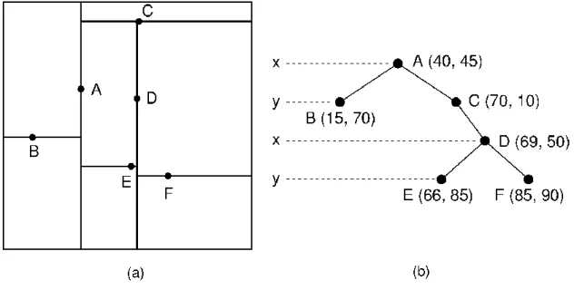
k-d tree is a classic search tree designed for multidimensional case [26]. It allows for both range searches and nearest neighbor queries, featuring logarithmic average com-plexity of insertions, deletions and retrievals (worst case is linear). The tree is construct-ed by recursively splitting the data space along dimensions; splitting points can be mean or median values of corresponding vector components. Nearest neighbors can then be retrieved by a procedure similar to depth-first search: the first leaf node reached is taken as a current best, and then other subspaces that can potentially contain closer points are inspected. Figure 1 shows the example of 2-d tree.

(11)

Figure 1. Example of k-d tree for 2-dimensional data. 1

The approach taken by k-d trees to split the search space has significant drawbacks. Recursive partitioning leads to exponentially growing number of regions as dimension-ality increases. The splitting points may be expensive to compute for large data sizes, and random sampling, which was introduced to mitigate this drawback, may result in suboptimal partitions. The k-d tree often fails to take advantage of possible internal data regularity, instead creating “dead” regions (containing no database points).

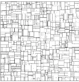
In an attempt to improve upon the k-d tree, many variants and modifications of it emerged over the years. Balltrees [27] represent a set hyperspheres instead of dimen-sional splits; these hyperspheres are not required to cover the data space completely and also allow regions to intersect or include each other. Vantage point tree (vp-tree) [28] further generalizes the problem to any metric space (instead of original Euclidean), per-forming splits based on similarity to a number of well-chosen vantage points. Figure 2 shows the k-d tree structure in comparison with vp-tree.

No matter what particular tree structure is used, some of their theoretical limitations cannot be overcome. Specifically, trees are not viable for high-dimensional data (𝐷 > 10). It has been demonstrated that in such scenarios they are reduced to exhaus-tive search with an additional overhead of maintaining the tree [5]. Query time therefore grows exponentially with dimensions; it is possible to make it polynomial, but only at the cost of making the preprocessing phase exponential instead [29]. Unfortunately, that makes trees unsuitable for many current applications; for example, the number of fea-tures in image or document retrieval easily reaches hundreds or thousands [30]. This shortcoming has become a large driving factor behind the recent large-scale research into approximate nearest neighbor techniques.

1

(12)

Figure 2.k-d tree space decomposition (left) and vp-tree decomposition (right). [28]

2.3 Hashing-based approximate search

In the context of ANN search, a hash function maps the original data space to another, significantly more limited space of hash codes [14]. The search problem becomes sig-nificantly easier to solve in the hash code space, allowing for a major computational gain. The approximate nature of the search stems from the imperfection of the hash function, as well as the inherent limitations of the new space.

Locality sensitive hashing (LSH) [25] is a family of hashing methods sharing the same design goal – similar items should be mapped to the same hash code (“bucket”) with a high probability, while dissimilar items should be placed in different buckets. Naturally, if this requirement is to be fulfilled, different hash functions are required for different similarity measures. Constructing distance-specific hash functions with theoretically guaranteed bounds of performance is an ongoing topic of extensive research. Numerous solutions have been proposed in the recent years, presenting LSH function families for distances such as 𝐿𝑝 (including e.g. Euclidean and Manhattan), cosine, Hamming, 𝜒2, as

well as rank similarity, Jaccard coefficient for sets and general non-metric distances [14].

LSH family methods require the entire database to be hashed and stored in a code table. Then fast ANN search can be performed by hashing the query, locating the correspond-ing bucket and retrievcorrespond-ing its contents (database vectors sharcorrespond-ing the same code) for a linear search. LSH thus does not reduce the costs of a distance computation, but instead makes the search non-exhaustive, effectively performing randomized space partitioning not unlike the previously considered tree structures.

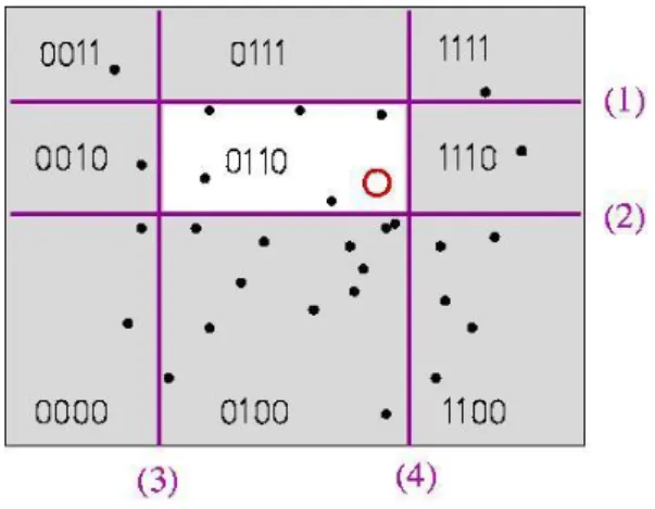
Figure 3 visually illustrates the concept. The red circle denotes the query, the hash code of which is “0110”. Only those database vectors that share the same code will be

(13)

re-was not hashed into the same bucket, leading to loss of search accuracy.

Figure 3.Visual example of locality sensitive hashing.2

To improve the search performance, it is common to use several hash functions simul-taneously [14]. For storage purposes the resulting codes are concatenated into a single vector, but during the retrieval the query is independently hashed with each function, and every corresponding bucket contributes its contents. The number of vectors for dis-tance calculation thus increases, but so does the accuracy.

One of the common LSH schemes for Euclidean distance is based on so-called 2-stable distributions [31]. An example of such a distribution is a Gaussian. The hash function is then given as

ℎ(𝑥) = ⌊𝑤𝑇_𝑟𝑥+𝑏⌋, (4)

where 𝑥 is a 𝐷-dimensional database vector, 𝑤 is a random 𝐷-dimensional vector sam-pled from the Gaussian distribution of zero mean and unit variance, 𝑟 is a positive real number and 𝑏 is an offset value, randomly chosen from a range [0, 𝑟]. The database vector is thus mapped to a single value via random projection and shifting.

Hash functions in the LSH family of methods are completely data-independent, making applications easier, but sacrificing performance. To alleviate this, several learning-to-hash approaches have been proposed [14]. They aim to derive and/or tune an efficient hash function from the specific data with respect to some optimization criterion, not unlike the training phase of machine learning models. A common secondary criterion is the maximization of the coding efficiency by maintaining bit balance and bit independ-ence. Bit balance implies that for each code bit the values 0 and 1 are approximately equally probable. Bit independence is hard to attain and is in practice relaxed to

2

(14)

relation; the purpose of both is minimizing the code redundancy. Together these re-quirements allow for the shortest codes possible given a particular data.

One influential example of an early data-specific hashing algorithm is spectral hashing

[32], which presents the similarities in a graph form and then infers binary codes as the balanced partitioning of the graph. Since the problem is NP-hard, it is solved approxi-mately by eigen-analysis of the graph Laplacian. To generalize the solution to the data not used for training, it is assumed that the input vectors are generated by the uniform distribution. Since this assumption is usually violated in practice, the performance of spectral hashing is degraded; the algorithm, however, provides important theoretical insights and has inspired many learning-to-hash approaches since.

Figure 4. ITQ on preprocessed normalized data. [33]

Iterative quantization (ITQ) [33] is an efficient learning-to-hash algorithm, which as-signs every database vector to a closest (in Euclidean terms) vertex of an 𝑀 -dimensional hypercube (𝑀 ≤ 𝐷). Every vertex can then be uniquely indexed by 𝑀 bits, resulting in binary hash codes. First the data dimensionality is reduced to 𝑀 via princi-pal component analysis (PCA). Then, to improve the hashing, rotation is applied to the preprocessed data, for the purpose of balancing the variances along each principal direc-tion. This corresponds to previously described bit balance requirement. Even the ran-dom rotation improves the hashing, but ITQ instead opts for an optimized rotation, giv-en the PCA-aligned data. This transformation is found by minimizing the Euclidean distance between each database vector and the hypercube vertex it is assigned to. The example can be seen on Figure 4. If no rotation is applied (Figure 4a), similar data points (contained in the same cluster) will be assigned to different hypercube vertices, resulting in different hash codes. Random rotation (Figure 4b) provides an improve-ment, but optimized rotation (Figure 4c) attains the best solution.

ITQ, as its name implies, is learned by an iterative procedure, alternating between as-signment of data points to vertices and optimizing the rotation. These two steps are re-peated until no further changes in hash codes occur.

(15)

3. VECTOR QUANTIZATION FOR APPROXIMATE

SEARCH

3.1 General concepts

Vector quantization (VQ) [16] is a technique that represents a given set of 𝑁 𝐷 -dimensional vectors with another set of 𝐾 centroids of the same dimensionality

(𝐾 < 𝑁). The set of centroids

𝐶

is called a codebook, while centroids themselves are alternatively called codevectors. Each vector from the original set is represented by one and only one codevector. Needless to say, VQ representation of the data is lossy. The quantization loss is typically measured by mean squared error (MSE) between the data vectors and their reproductions:

𝐸 =

1

𝑁

∑

‖𝑞(𝑥) − 𝑥‖

2 2 𝑁

𝑖=1

,

(5)

where 𝑥 is the data vector and 𝑞(𝑥) is the corresponding codevector.

Any optimal (having minimal quantization loss) VQ quantizer is subject to two neces-sary optimality conditions, known as Lloyd conditions [17]. First condition states that each vector must be assigned to a centroid which is the closest in Euclidean distance terms:

 

2 2

ar

g min

.

i i c C

q x

c

x







₍₆₎

Second condition limits the position of each centroid to the mean value of all the vectors it represents:

𝑐_𝑖 =_𝑛1

𝑖∑ 𝑥𝑗

𝑛_𝑖

𝑗=1 , 𝑠. 𝑡. 𝑞(𝑥𝑗) = 𝑐𝑖 (7)

These conditions are greatly reminiscent of well-known k-means clustering. Indeed, a common way to construct a vector quantizer is with a Lloyd’s algorithm:

1. Randomly initialize centroid positions.

2. Repeat for a predetermined number of iterations:

a. Assign every data vector to the nearest centroid (6).

(16)

The total computational complexity of Lloyd’s algorithm is 𝑂(𝐿𝑁𝐾𝐷), where 𝐿 is the number of iterations. While Lloyd’s algorithm is intuitive, simple and widely used, it only converges to a locally optimal solution. The results may vary wildly with different initializations, and some starting points may lead to very poor representations.

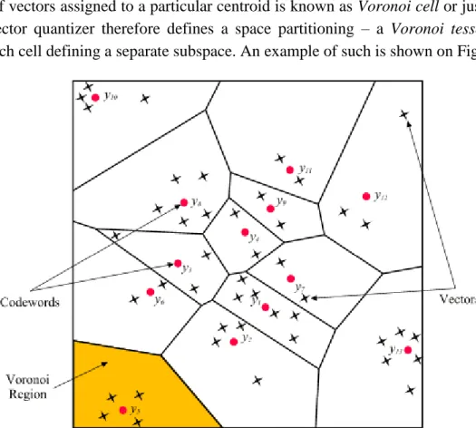
A set of vectors assigned to a particular centroid is known as Voronoi cell or just a cell. Any vector quantizer therefore defines a space partitioning – a Voronoi tessellation, with each cell defining a separate subspace. An example of such is shown on Figure 5.

Figure 5. An example of a vector quantizer and corresponding Voronoi tesselation.3

Evidently, the Voronoi tessellation can be used as a foundation for non-exhaustive dis-tance calculation. One strong advantage of such an approach, when compared to hash-ing, would be the fact that the original data space is preserved, and the Euclidean dis-tances remain meaningful instead of being approximated with Hamming disdis-tances. Bet-ter preservation of pairwise vector dissimilarities, in turn, leads to betBet-ter search perfor-mance.

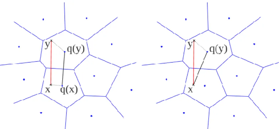
Since vector quantization does not change the distance function, there are two possible approaches to the nearest neighbor search [18]. If symmetric distance computation

(SDC) is used, the query vector is quantized to the nearest centroid, and then the dis-tances from that centroid to all the others are estimated. In case of asymmetric distance computation (ADC), the distances between the query and all the centroids are calculated directly. Both scenarios are shown on Figure 6.

3

(17)

Figure 6.Distance computation with vector quantization: symmetric (left) and asymmetric (right). [18]

Since centroid positions are always known in advance when the search is performed, it is possible to precompute all the pairwise distances between centroids and store them. This seemingly makes SDC very quick, but to quantize the query, one needs to calculate the distance from it to every centroid, which is the exact same process as in ADC. As a result, the differences in the calculation speed between the two are minimal. However, the quantization of the query vector introduces additional distortion. It is thus reasona-ble to conclude that ADC is superior to SDC and should be preferred. In fact, availabil-ity of ADC is a direct consequence of space preservation and can be considered an addi-tional advantage of vector quantization over hashing-based approaches.

Despite the aforementioned benefits, traditional vector quantization without any chang-es is not a practical solution for approximate nearchang-est neighbor search, as it too suffers from the “curse of dimensionality” [18][34]. If the number of codevectors (centroids) is

𝐾, the code (index) of each database vector has a length of log₂𝐾 bits. This is not near-ly enough for discrimination; for example, if a vector of dimensionality 960 (e.g. global color GIST descriptor [35]) would be represented by a 960-bit code (1 bit per dimen-sion), the corresponding vector quantizer would have to have 2960 centroids. Evidently, it is impossible to even store a codebook of that size in a computer memory, let alone applying any search operations on it. A different approach is necessary to take ad-vantage of VQ properties. A number of such approaches have emerged, proceeding to outperform hashing-based techniques by a large margin [18][19][20].

3.2 Product quantization (PQ)

Product quantization (PQ) [18] is one of the most important methods in the vector quantization family. To allow for more powerful representations with small number of codevectors, PQ splits the data space into 𝑀 subspaces, each of 𝐷 𝑀⁄ dimensions. Vec-tor quantization (learned with Lloyd’s algorithm) is then separately applied on each

(18)

subspace, resulting in 𝑀 codebooks. Every database vector can be subsequently recon-structed by concatenating 𝑀 corresponding codevectors. Assuming that each codebook has 𝐾 codevectors, the total number of possible representations is 𝐾𝑀. Any quantized database vector is stored as a sequence of 𝑀 codes, indexing into 𝐾 elements each, re-sulting in a total code length of 𝑀 log₂𝐾 bits. The amount of memory required for codebook storage (in terms of scalar values) is 𝑀 ∙ 𝐾 ∙_𝑀𝐷 = 𝐾𝐷, which is small in prac-tice, as 𝐾 ≪ 𝑁.

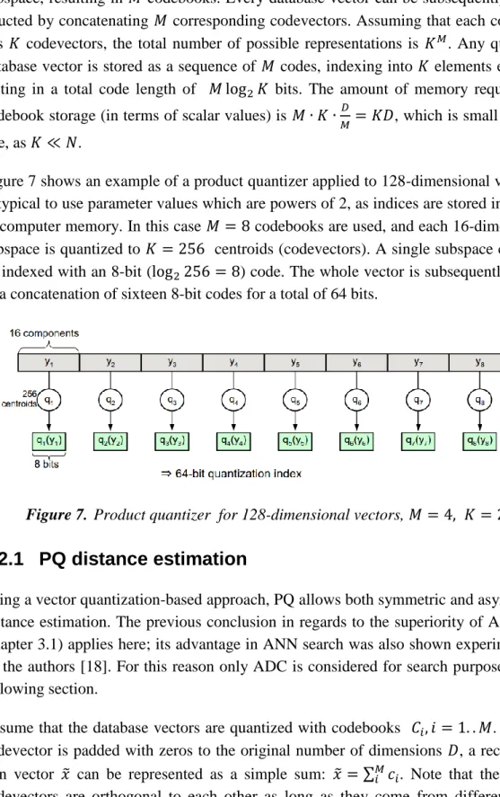
Figure 7 shows an example of a product quantizer applied to 128-dimensional vector. It is typical to use parameter values which are powers of 2, as indices are stored in a bina-ry computer memobina-ry. In this case 𝑀 = 8 codebooks are used, and each 16-dimensional subspace is quantized to 𝐾 = 256 centroids (codevectors). A single subspace can then be indexed with an 8-bit (log₂256 = 8) code. The whole vector is subsequently stored as a concatenation of sixteen 8-bit codes for a total of 64 bits.

Figure 7. Product quantizer for 128-dimensional vectors, 𝑀 = 4, 𝐾 = 256.4

3.2.1 PQ distance estimation

Being a vector quantization-based approach, PQ allows both symmetric and asymmetric distance estimation. The previous conclusion in regards to the superiority of ADC (see Chapter 3.1) applies here; its advantage in ANN search was also shown experimentally by the authors [18]. For this reason only ADC is considered for search purposes in the following section.

Assume that the database vectors are quantized with codebooks 𝐶_𝑖, 𝑖 = 1. . 𝑀. If every codevector is padded with zeros to the original number of dimensions 𝐷, a reconstruc-tion vector 𝑥̃ can be represented as a simple sum: 𝑥̃ = ∑ 𝑐𝑀𝑖 𝑖. Note that the padded

codevectors are orthogonal to each other as long as they come from different code-books. Then the squared Euclidean distance between 𝑥̃ and a query vector 𝑞 decompos-es to the sum of distancdecompos-es over the individual subspacdecompos-es:

‖𝑞 − 𝑥̃‖22 = ∑ ‖𝑞 − 𝑐𝑀𝑖 𝑖‖22− (𝑀 − 1)‖𝑞‖22 (8)

4

(19)

unless the estimated values of distances are required. Taking into account the codevec-tor structure, the total number of operations required to compute (8) is 𝑂(𝑀 ∙_𝑀𝐷) =

𝑂(𝐷) – the same as if the distance was computed without quantization. The benefit of PQ is in the fact that the same set of codevectors is used to represent the whole original database.

It is possible to compute pairwise distances between a given query vector and all the codevectors (from all codebooks), storing them into a table. This would require

𝑀 ∙ 𝐾 ∙_𝑀𝐷 = 𝐾𝐷 operations, taking subspaces into account. Then the value of ‖𝑞 − 𝑐_𝑖‖₂2 can be found in constant time via a table lookup, meaning that ‖𝑞 − 𝑥̃‖₂2 can be calcu-lated in 𝑀 lookups and 𝑀 summations. Estimating the distances from the given query to a quantized set of 𝑁 vectors would require 𝑂(𝐾𝐷 + 𝑁𝑀) total operations. This is sig-nificantly smaller than the linear search of 𝑂(𝑁𝐷). Since the dimensionality and num-ber of vectors are decoupled, product quantizer allows for much better scaling on both. One drawback of such an approach is the exhaustive nature of the search. When 𝑁 is very large, even the product quantizer costs may become excessive. Inverted indexing is one of the possible solutions for this problem [18]. Simple vector quantization is applied on the data, with a number of centroids 𝑘′ < 𝑁 ≪ 𝐾𝑀. The value of 𝑘′ typically ranges anywhere from 103 to 106. Then for each data point the residual is calculated between it and the centroid of its cell:

𝑟(𝑥) = 𝑥 − 𝑞(𝑥) (9)

These residuals are subsequently quantized with PQ, and both representations are re-tained. When the query is processed, the centroids of the coarse quantizer (VQ) are ex-haustively searched first, requiring 𝑂(𝑘′𝐷) operations. When the nearest centroid is located, query residual is computed and the normal PQ distance estimation is per-formed, but only in a single Voronoi cell, which contains some subset of the database. This allows for significant search speedup at the cost of additional memory require-ments [18]. Although it’s possible to learn a separate product quantizer in each Voronoi cell, this would be prohibitive for large 𝑘′, meaning that a single set of PQ codebooks is used for all the residuals. Additional memory costs are thus 𝑂(𝑘′𝐷) to store the coarse quantizer and 𝑂(𝑁 log₂𝑘′) for all the corresponding indices.

It is common in practice that the database vector and its true nearest neighbor would be assigned to the separate centroids of the coarse quantizer. This means that the procedure outlined above could not possibly locate the true neighbor, as it is not included in the data subset to be searched. To alleviate this, a multiple assignment strategy is proposed [18][36]. During the coarse quantization step, each database vector is assigned not to a

(20)

single closest centroid, but to 𝑤 nearest centroids. All of their contents are consequently retrieved for exhaustive searching. The PQ authors have concluded that inverse index-ing with multiple assignment provides a major speedup for large databases and even improves the search performance in some cases [18].

3.2.2 Learning the product quantizer

To encode a data vector with PQ (given a set of codebooks), it is necessary to locate the closest centroid (in Euclidean terms). PQ centroids are generated by the Cartesian prod-uct of the codebooks, so the total number of options is, as mentioned earlier, 𝐾𝑀. This is too large for an exhaustive search. Fortunately, subspace orthogonality can be exploited here, same as for the query distance estimation. The distance between a given vector and a PQ centroid decomposes into the sum of distances to codevectors within individu-al subspaces, yielding the exact same result as (8). The nearest neighbor search in 𝐾𝑀 vectors is thus replaced with 𝑀 nearest neighbor searches in 𝐾 vectors each; the indices of the located codevectors are then concatenated to obtain the result. Computational complexity of encoding a single vector becomes 𝑂 (𝑀 ∙ 𝐾 ∙_𝑀𝐷) = 𝑂(𝐾𝐷). It is im-portant to note that encoding costs do not depend on the number of codebooks 𝑀. Before PQ can be applied on a dataset, it is necessary to obtain a good set of codebooks. Because the codebooks are data-specific, they need to be learned in a process known as

training. Product quantization inherits its training scheme directly from vector quantiza-tion, adapting a simple Lloyd algorithm for iterative adaptation. To save computation time, it is common to not use the whole data for training, opting instead for a repre-sentative subset.

As discussed earlier, Lloyd’s algorithm alternates between centroid assignment and cen-troid adjustment. The former corresponds to encoding the training data, which was al-ready described. The latter involves adapting the codebooks to minimize the quantiza-tion error, given a particular encoding of the data. As PQ is equivalent to VQ in each individual subspace, optimal codevectors are generated by averaging their correspond-ing Voronoi cells. PQ traincorrespond-ing is thus completely equivalent to runncorrespond-ing 𝑀 k-means clus-tering algorithms in reduced dimensionality spaces. With 𝐿 training iterations and 𝑁 training vectors, the total complexity of learning a set of codebooks is 𝑂(𝑁𝐿𝐾𝐷). To start the training, it is necessary to define a starting point – either an initial encoding or an initial set of codebooks. Although it’s possible to use random (e.g. uniform) codes for this purpose, the common approach is to generate the codevectors by sampling from the corresponding dimensions of training data [18].

(21)

Optimized product quantization (OPQ) [19], also known as Cartesian k-means (CKM)

[37], is a variant of product quantization that makes an attempt to optimize the alloca-tions of dimensions to subspaces. In the original PQ paper [18] it was noted that the search performance varies greatly based on the contents (semantics) of the data. Product quantization considers all the subspaces to be equal in terms of information content, which is quite likely to be incorrect for the real sets of vectors. In fact, the choice of dimensions for a particular subspace has been shown to have a major effect on the quan-tization performance [18]. Since the domain knowledge is not always available, the quantization algorithm can benefit from an internal subspace optimization.

Rotation is a linear transformation that preserves vector norms and pairwise Euclidean distances; for any orthogonal 𝐷 × 𝐷 matrix 𝑅 and 𝐷-dimensional vectors 𝑥 and 𝑦 the following expression holds:

‖𝑥 − 𝑦‖₂2 _{= ‖𝑅𝑥 − 𝑅𝑦‖} 2

2_. ₍₁₀₎

Due to (10) any centroid assignments (codes) of a vector quantizer with codebook 𝐶 on dataset 𝑋 remain valid, if both codevectors and data vectors are transformed with the same matrix 𝑅. This property naturally generalizes to PQ. The benefit of rotation lies in the fact that it can represent any reordering of the vector dimensions [19]. Optimizing rotation of PQ quantizer is thus equivalent to finding better allocation of dimensions to subspaces. Random rotation has been explored and found to improve the quantization error and search performance [38]. Further gains can be expected if the matrix 𝑅 is fine-tuned with respect to the data.

OPQ differs from PQ in that it learns not only codebooks and codes, but also an orthog-onal transformation matrix 𝑅. Any data to be encoded is first rotated via multiplication by 𝑅, and then the product quantizer is applied. Computational complexity of encoding a single vector thus increases by the multiplication cost, resulting in a total estimate of

𝑂(𝐾𝐷 + 𝐷2₎_.

Two formulations of OPQ exist [19]. Parametric formulation is derived from the as-sumption that the data is generated by Gaussian distribution. If the asas-sumption holds, the solution is provably optimal and achieves the theoretical lower bound of quantiza-tion error, which is derived to be

𝐸 ≥ _𝑀𝐷𝐾−2𝑀𝐷 ∑ |Σ̂_𝑚| 𝑀 𝐷

𝑀

𝑚=1 , (11)

where Σ̂_𝑚 is the covariance submatrix of 𝑚-th subspace of rotated data 𝑅𝑥. Further the-oretical analysis shows that for a parametric solution to achieve optimality, two condi-tions must hold: subspace independence and balance of subspace variance. These

(22)

con-clusions exactly correspond to the ones drawn in ITQ – a hashing-based method de-scribed earlier.

To construct a matrix R satisfying the above requirements for subspaces, a simple greedy algorithm – eigenvalue allocation – was proposed [19]. The database is first processed with PCA, which takes 𝑂(𝑁𝐷2+ 𝐷3) operations. The eigenvalues are then sorted in a descending order and sequentially allocated to 𝑀 bins of capacity 𝐷 𝑀⁄ , such that the product of values inside each bin would be roughly equal (thus balancing the variance). When the eigenvectors are reordered according to allocation of their respec-tive eigenvalues, the matrix 𝑅 is formed. Then the database is rotated and PQ is applied on the result. Total training complexity of parametric OPQ is thus 𝑂(𝑁𝐷2+ 𝐷3 +

𝑁𝐿𝐾𝐷).

Naturally, the Gaussian assumption rarely holds in practice. Nonparametric OPQ does not construct a single rotation matrix, but instead optimizes it during the training phase [19]. At the beginning of each iteration the data is rotated with the current estimate of 𝑅. Then the codebook adaptation and encoding are performed on the rotated data, with no differences from PQ. Finally, the current estimate of 𝑅 is updated so as to minimize the quantization error criterion:

2

min _F,

R RX Y (12)

where 𝑋 and 𝑌 are matrices composed of original (not rotated) data vectors and their reconstructions, respectively, and ‖∙‖_𝐹 is the Frobenius norm: ‖𝐴‖_𝐹 = √𝑡𝑟𝑎𝑐𝑒(𝐴∗𝐴). To solve this optimization problem, first the singular value decomposition (SVD) of

𝑋𝑌𝑇_{is calculated:}_𝑋𝑌𝑇 _{= 𝑈𝑆𝑉}𝑇_{. The matrix}_𝑅_{is then calculated as follows:}

𝑅 = 𝑉𝑈𝑇_. ₍₁₃₎

The complexities of this procedure are as follows: 𝑋𝑌𝑇 multiplication is 𝑂(𝑁𝐷2), SVD is 𝑂(𝐷3), and 𝑉𝑈𝑇 multiplication is also 𝑂(𝐷3). Since rotation is adapted in each itera-tion, the total cost of non-parametric OPQ training becomes 𝑂(𝐿(𝑁𝐾𝐷 + 𝑁𝐷2+ 𝐷3)). Nonparametric OPQ typically performs better on real datasets, as it does not rely on Gaussian assumption. OPQ training can be initialized similarly to PQ, with an identity matrix as a first estimate of 𝑅. Better results are attained if parametric solution is used for initialization, although that increases the amount of computation required [19].

(23)

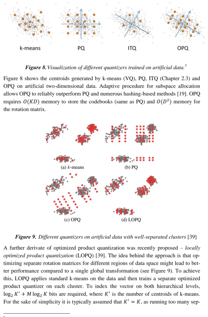
Figure 8.Visualization of different quantizers trained on artificial data.5

Figure 8 shows the centroids generated by k-means (VQ), PQ, ITQ (Chapter 2.3) and OPQ on artificial two-dimensional data. Adaptive procedure for subspace allocation allows OPQ to reliably outperform PQ and numerous hashing-based methods [19]. OPQ requires 𝑂(𝐾𝐷) memory to store the codebooks (same as PQ) and 𝑂(𝐷2) memory for the rotation matrix.

Figure 9. Different quantizers on artificial data with well-separated clusters [39] A further derivate of optimized product quantization was recently proposed – locally optimized product quantization (LOPQ) [39]. The idea behind the approach is that op-timizing separate rotation matrices for different regions of data space might lead to bet-ter performance compared to a single global transformation (see Figure 9). To achieve this, LOPQ applies standard k-means on the data and then trains a separate optimized product quantizer on each cluster. To index the vector on both hierarchical levels,

log₂𝐾′_{+ 𝑀 log}

2𝐾 bits are required, where 𝐾′ is the number of centroids of k-means.

For the sake of simplicity it is typically assumed that 𝐾′= 𝐾, as running too many

5

(24)

arate OPQ algorithms will increase the computational costs dramatically. Assume that the top-level quantizer is learned over 𝐿′ iterations, and the data is roughly equally dis-tributed between k-means clusters. Then it takes 𝑂(𝐿′𝐾𝑁𝐷) operations to run global k-means, followed by the costs of training 𝐾 OPQ instances on 𝑁 𝐾⁄ data points each, which is 𝑂(𝐾𝐿(𝑁𝐷 + 𝑁𝐷2+ 𝐷3)). Adding the two together and simplifying the result leads to the following LOPQ training complexity: 𝑂(𝐿′𝑁𝐾𝐷 + 𝐿𝐾(𝑁𝐷2+ 𝐷3)). In addition to the training overhead, other operations with LOPQ naturally have higher computational costs. 𝐾 individual OPQ quantizers need to be stored, resulting in memory cost of 𝑂(𝐾𝐷[𝐾 + 𝐷]). Query processing requires searching the top level first, which takes extra 𝐾𝐷 operations, but the following OPQ distance estimation is non-exhaustive and takes 𝐷2+ 𝐾𝐷 + 𝑁′𝑀 operations, where 𝑁′< 𝑁. Finally, a vector encoding cost also increases by 𝐾𝐷 operations due to the need of locating the closest top-level centroid.

LOPQ requires noticeably more complex training, but its encoding and distance calcula-tion overheads, as well as increase in code length, are considered to be well justified by the improvement in quantization error and search performance [39].

3.3 Additive quantization (AQ)

Additive quantization (AQ) generalizes the methods described earlier by relaxing code-book constraints [21]. The quantizer, similarly to PQ or OPQ, consists of 𝑀 codebooks, each containing 𝐾 codevectors. However, no subspace decomposition is performed, and all the codevectors share the same dimensionality 𝐷 as the original data. Instead of con-catenation, 𝑀 indexed codevectors are instead added together to obtain a reconstruction (see Figure 10).

(25)

The representation codelength is still 𝑀 log2𝐾, just as in the methods of PQ family.

Memory requirements for codebook storage are naturally higher, due to the increased codevector dimensionality, and constitute an equivalent of 𝑀𝐾𝐷 values – 𝑀 times larg-er when compared to PQ or OPQ. Since the value of 𝑀 is rarely above 16, this extra cost is deemed negligible for sufficiently large datasets. Any set of PQ or OPQ code-books may be converted to a set of AQ codecode-books by appropriate padding of all codevectors with zeroes.

Elimination of subspace decomposition means the omission of codebook orthogonality constraint. This, in turn, leads to potentially richer representation, and AQ indeed has outperformed older methods significantly [21]; however, this formulation comes with the price of much higher encoding and training complexity, as simple k-means proce-dure is no longer applicable.

3.3.1 AQ distance estimation

The squared Euclidean distance from query 𝑞 to a reconstructed vector 𝑥̃ = ∑𝑀_𝑖=1𝑐_𝑖 can be represented with the following expression:

𝑑𝑖𝑠𝑡2_{(𝑞, 𝑥̃) = ∑ ‖𝑞 − 𝑐} 𝑖‖22 𝑀

𝑖=1 − (𝑀 − 1)‖𝑞‖22+ ∑𝑀𝑖=1∑𝑀𝑗=1,𝑖≠𝑗⟨𝑐𝑖, 𝑐𝑗⟩ (14)

When compared to (8), AQ distance estimate has an additional component – the sum of dot products between all the included codevectors. This is due to codebooks no longer being orthogonal. Since this component does not depend on 𝑞, it can be precomputed and reused for different queries. One approach is to construct a set of lookup tables, containing dot products between all the possible pairs of codevectors. In this case 𝑀2⁄2 extra lookups will be required for every search, in addition to 𝑂(𝑀2𝐾2) memory. An-other solution would be to calculate the sum in (14) for each encoded vector in the data-base and store it as set of scalars. To reduce the memory overhead, these scalar values can be quantized and appended to the AQ code of each data point; then the dot products in (14) can be found with a single lookup. Although this operation further distorts the distances and degrades the search performance, experiments have shown that the detri-mental effects are minimal and may well be justified by the faster search [21].

The first two terms of (14) are identical to their PQ equivalents. The only difference is that full-length codebooks result in more expensive lookup table calculations –

𝑂(𝑀𝐾𝐷) instead of 𝑂(𝐾𝐷). However, since 𝑀 is relatively small in practice (rarely taking a value above 𝑀 = 16), this overhead is considered acceptable, especially for large databases [21]. The total search cost for a single query therefore becomes

(26)

3.3.2 Learning the additive quantizer

An additive quantizer is trained iteratively, via alternating between codebook adaptation and encoding. Unfortunately, the distance estimate of (14) is more complex than (8), so a simple problem decomposition is not possible; general approaches for both of the steps need to be devised instead.

Given fixed codes, an optimal set of codebooks can be found by solving the following least-squares problem:

min

_𝐶_𝑚𝑘

∑ ‖𝑥

_𝑛

− ∑ ∑ 𝑎

𝑀 𝐾_𝑘 _𝑛𝑚𝑘

𝐶

_𝑚,𝑘

𝑚

‖

₂2

𝑁

𝑛

,

(15)

_{𝑚,𝑘𝐷}

= 𝑥

𝑁𝐷 (16)

Fortunately, since only 𝑀 out of 𝑀𝐾 coefficients in each equation are nonzero, the co-efficient matrix can be co-efficiently stored in sparse format (with density 1 𝐾⁄ ), allowing for special solvers to be used. In addition, the coefficient matrix is exactly the same for all the systems (only the right-hand constant terms 𝑥_𝑖𝑑 change), so it can be reused for all the solutions. These factors lead the AQ authors to disregard the computational costs of codebook adaptation during training, as the complexity is dominated by the encoding step [21].

The problem of finding the optimal AQ representation of a given vector is equivalent to inference on a fully connected pairwise Markov Random Field (MRF), which is NP-hard [21][40]. One of the simplest algorithms for this problem is Iterated Conditional Modes (ICM) [41]. In the context of AQ encoding ICM proceeds as follows:

1. Given a database vector 𝑥, set iteration counter 𝑙 = 1, current reconstruction

𝑥̃ = 0 and codevector assignments 𝑖𝑚 = 0, 𝑚 = 1 … 𝑀

.

2. For all the codebooks 𝑚 = 1 … 𝑀 do:

a. If 𝑖𝑚≠ 0, subtract the currently assigned codevector from the

recon-struction: 𝑥̃ = 𝑥̃ − 𝐶_𝑚,𝑖_𝑚.

(27)

𝑖_𝑚 = arg min‖𝑟 − 𝐶_𝑚,𝑖_𝑚‖₂2 (17) d. Modify the reconstruction accordingly: 𝑥̃ = 𝑥̃ + 𝐶_𝑚,𝑖_𝑚 and proceed to

the next codebook.

3. Increase the iteration counter 𝑙 = 𝑙 + 1, if pre-specified maximal number of iterations 𝐿 was reached, stop, otherwise go to step 2.

As can be seen from the above, ICM considers one codebook at a time and tries to im-prove the quantization error, while keeping other 𝑀 − 1 assignments fixed. This solu-tion has a complexity of 𝑂(𝐿𝑀𝐾𝐷) for encoding a single vector; unfortunately, as it never considers interaction between codebooks, its greediness leads to poor practical performance. Other MRF-specific methods were also considered by the AQ authors, but failed to achieve suitable results, prompting them to suggest their own approach [21].

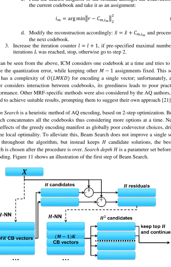
Beam Search is a heuristic method of AQ encoding, based on 2-step optimization. Beam Search concatenates all the codebooks thus considering more options at a time. Nega-tive effects of the greedy encoding manifest as globally poor codevector choices, driven by the local optimality. To alleviate this, Beam Search does not improve a single solu-tion throughout the algorithm, but instead keeps 𝐻 candidate solutions, the best of which is chosen after the procedure is over. Search depth𝐻 is a parameter set before the encoding. Figure 11 shows an illustration of the first step of Beam Search.

Figure 11. Visual representation of the first iteration of Beam Search encoding.

(28)

1. Given a database vector 𝑥 and search depth 𝐻, set codevector assignments

𝑖_𝑚 = 0, 𝑚 = 1 … 𝑀

.

2. Find 𝐻 nearest neighbors to 𝑥 from all the 𝑀𝐾 codevectors and store them, as well as corresponding codebook indices, as candidate solutions:

𝐼 = {{𝑚̅1, 𝑖𝑚̅1} {𝑚̅2, 𝑖𝑚̅2} … {𝑚̅𝐻, 𝑖𝑚̅𝐻}}.

Here 𝑚̅_𝑗 is a set of codebook indices and 𝑖_𝑚_̅_𝑗 is a set of corresponding codevector assignments.

3. For every candidate solution 𝐼_ℎ, ℎ = 1 … 𝐻 do: a. Calculate the solution residual:

𝑟 = 𝑥 − ∑ 𝐶_𝑚 _𝑚,𝑖_𝑚, 𝑚 ∈ 𝑚̅_ℎ.

b. Find 𝐻 nearest neighbors 𝑖_𝑚∗ to 𝑟 from 𝐶′= ⋃ 𝐶𝑚, 𝑚 ∉ 𝑚̅_ℎ, i.e. from all codevectors whose codebooks are not yet in the solution. c. Generate 𝐻 new solutions by appending the indices found in the

pre-vious step to the current solution:

𝑚̅ℎ𝑗 = 𝑚̅ℎ∩ 𝑚𝑗∗, 𝑖𝑚̅ℎ𝑗 = 𝑖𝑚̅ℎ ∩ 𝑖𝑚𝑗∗, 𝑗 = 1 … 𝐻.

d. Replace the current solution with 𝐻 newly generated ones:

𝐼 = 𝐼 ∖ {𝑚̅_ℎ, 𝑖_𝑚_̅_ℎ} ∩ {𝑚̅_ℎ1, 𝑖_𝑚_̅_ℎ1} ∩ … ∩ {𝑚̅_ℎ𝐻, 𝑖_𝑚_̅_ℎ𝐻}

4. 𝐼 is now a list of 𝐻2 solutions. Sort the list by the quantization error and keep

𝐻 best solutions.

5. If every solution in 𝐼 contains 𝑀 codevectors, take the solution with the low-est quantization error as a final answer and stop. Otherwise go to step 3. Two-step optimization allows Beam Search encoding to find significantly better repre-sentations. The major drawback lies in the complexity of the procedure. The algorithm described above has the complexity of 𝑂(𝑀3𝐾𝐻𝐷), which is the highest amongst the current quantization-based approaches. Some improvement can be attained by avoiding the distance calculations within the encoding process, replacing them with table lookups. The table can be constructed in 𝑂(𝑀𝐾𝐷), resulting in a total complexity of

𝑂(𝑀3_{𝐾𝐻 + 𝑀𝐾𝐷)}_{. In this case the data dimensionality has a lesser effect on encoding,}

but the cost remains very high. It is particularly pronounced during the training phase, where the dataset has to be repeatedly re-encoded over several iterations.

AQ with Beam Search encoding has demonstrated superior results in both search and quantization error reduction, improving upon the majority of other methods [21]. How-ever, the prohibitive complexity hinders the practicality of AQ applications. Training time is typically given less consideration in ANN search systems, as it is performed in offline mode and can be assumed to take advantage of the full computational power available. Encoding new database vectors, on the other hand, is a relatively common task and can be considered time-sensitive.

AQ authors suggest a simple approach to slightly reduce the computational costs of AQ while sacrificing some representation power. As AQ scales cubically with the number of codebooks, it may be viable to perform explicit subspace decomposition similar to PQ and apply a separate AQ quantizer in each subspace. Optimal rotation of OPQ may be applied to improve the allocations of dimensions in such case. This simple technique

(29)

if the decomposition is performed with 𝑆 subspaces and 𝑀′ < 𝑀 codebooks are used in each, the requirement becomes 𝑆 (𝑀′𝐾𝐷_𝑆) = 𝑀′𝐾𝐷, plus 𝐷2 (optionally) for the rota-tion matrix. APQ is quite commonly used instead of AQ in experiments with extremely large data (billions of vectors) or with high numbers of codebooks (𝑀 ≥ 16).

3.3.3 Derivate methods

Several AQ derivate methods have been recently proposed [22][23]. While sharing the same representation and overall approach, these methods impose certain constraints on the codebooks, limiting the search space of encoding. This allows for significantly fast-er training and processing, making these solutions more practical. The cost of simplifi-cation is degradation in search performance, caused by the loss of generality. One such approach is described here to give an example of the tradeoff.

Composite quantization (CQ) [22] was first formulated in an attempt to simplify AQ distance calculations. As mentioned earlier, AQ distance estimate (14) differs from the one used in PQ (8) due to the presence of nonzero dot products between the codevec-tors. This scalar value could either be precomputed (and optionally quantized) or calcu-lated during the search, requiring 𝑀2⁄2 additional lookups. Composite quantization imposes the following constraint: for any set of 𝑀 codevectors, each coming from a different codebook, their dot products have to sum up to a single constant value 𝜖:

∀𝑐₁ ∈ 𝐶₁, 𝑐₂ ∈ 𝐶₂… , 𝑐_𝑀 ∈ 𝐶_𝑀: ∑ ∑𝑀 ⟨𝑐_𝑖, 𝑐_𝑗⟩ 𝑗=1,𝑖≠𝑗 𝑀

𝑖=1 = 𝜖 (18)

In this case the corresponding component in (14) can be disregarded during the search, as it value is independent of both the query and the encoded data. Distance estimation then requires only 𝑀 lookups from a query-specific table.

Besides the above simplification, CQ constraint carries a more important consequence. If it is perfectly satisfied, the reconstruction error of any database vector, which follows the same expression as (14), decomposes to sum of errors for individual codevectors. The encoding can then be performed in the same manner as PQ – by a series of inde-pendent nearest neighbor searches within each codebook. Still, even if 𝜖 = 0, CQ re-mains more general than PQ, as no explicit subspace decomposition is performed and codebooks can be any orthogonal vector sets.

To satisfy the CQ constraint, the codebook adaptation procedure must be changed. The new error function is obtained by adding a quadratic penalty on constraint violation. Reformulated optimization problem of CQ training is given as follows:

(30)

min𝐶,𝑎,𝜖∑ ‖𝑥𝑛− ∑ 𝑐𝑀𝑖 𝑛𝑖‖₂ 2 + 𝜇 ∑ (∑ 〈𝑐𝑀𝑖≠𝑗 𝑛𝑖, 𝑐𝑛𝑗〉 − 𝜖) 2 𝑁 𝑛 𝑁 𝑛 , (19)

where 𝜇 is the penalty parameter chosen via cross-validation. Since this is a complex problem with no closed-form solution, trained composite quantizer will not exactly ful-fill the CQ constraint in practice. Still, it is assumed that the solution is close to optimal and dropping the dot products in distance estimation (14) will not introduce significant errors.

Composite quantizer is trained by alternating between the following three steps:

1. Updating assignments, i.e. encoding the training set with current codebooks and fixed 𝜖. Due to CQ constraint not being perfectly realized, independent codebook searches (akin to PQ) would produce suboptimal results, which can potentially propagate through training iterations. For this reason ICM (see Section 3.3.2) is adopted, as a compromise between simplicity and quality. However, instead of simple distances, (19) is used as a minimization criterion for choosing the codevectors. The complexity of this step is 𝑂(𝐿𝑁𝑀𝐾𝐷); au-thors suggest the number of ICM iterations 𝐿 = 3.

2. Updating 𝜖, given fixed codebooks and encoding. From (19) it trivially fol-lows that an optimal value for 𝜖 is an average sum of dot products over the training set:

𝜖 =_𝑁1∑ ∑ 〈𝑐𝑀 _𝑛𝑖, 𝑐_𝑛𝑗〉 𝑖≠𝑗

𝑁

𝑛 (20)

The complexity of this update is 𝑂(𝑁𝑀2), assuming that the dot products have been precomputed and stored in a lookup table.

3. Updating codebooks, given encoding and 𝜖. This is an unconstrained nonlin-ear optimization problem. CQ authors suggest the use of quasi-Newton solv-ers and specifically refer to L-BFGS, which has publicly available implemen-tations [22].The complexity of this step is 𝑂(𝑁𝑀𝐷𝑇_𝑙𝑇_𝑐), where 𝑇_𝑐 is the number of L-BFGS iterations and 𝑇𝑙 is a number of line searches within

L-BFGS; CQ authors suggest 𝑇_𝑐 = 10 and 𝑇_𝑙 = 5.

At the beginning of each training iteration the dot products have to be computed and stored in a lookup table, to allow for fast objective function evaluation. The total as-ymptotic complexity of CQ training is thus 𝑂(𝑀2𝐾2𝐷 + 𝑁𝑀𝐾𝐷 + 𝑁𝑀2).

For CQ there is no need to store dot product lookup tables or quantize the corresponding value, leading to some memory savings when compared to AQ. The two approaches are otherwise almost identical from the application viewpoint, after the training has been performed. However, CQ, unlike AQ, allows for fast vector encoding with ICM, which allows for smaller computational expenses of growing the database.

While the constraint on dot products reduces the representational ability of the quantiz-er, negatively affecting its performance metrics, it also allows for faster lookups and

(31)

Tree quantization (TQ) [23] is a direct successor to AQ, imposing very particular or-thogonality constraints to make exact (optimal) encoding possible. In PQ a single di-mension was represented by only one codebook, while in the opposite case of AQ it was represented by all the codebooks. TQ employs a compromise solution instead: every dimension is encoded exactly twice (see Figure 12).

Figure 12. Representation of TQ encoding with 8 codebooks [23].

Underlying constraints are expressed with a tree structure, the so-called coding tree, where every node is a codebook and every edge corresponds to one or more data dimen-sions. Each codebook only contains dimensions that are mapped to its adjacent edges in the graph. It follows that any pair of codebooks which are not immediate neighbors in the tree are orthogonal. TQ thus performs subspace decomposition, but the one that is more general in nature.

While AQ encoding is equivalent to inference on fully connected MRF, TQ corresponds to its Chow-Liu approximation [23]. Exact solution can be calculated for the latter in polynomial time; in practice this translates to 𝑂(𝑀𝐾2) encoding complexity. Another benefit is that during the distance estimation, the dot product component of (14) can be calculated in linear time, only being nonzero for the codebooks adjacent in the tree. Similarly to CQ, TQ training scheme has to be extended to accommodate for con-straints. Between the encoding, which is done with exact inference on the graph, and the codebook adaptation, which does not differ from AQ, the coding tree itself needs to be constructed. A complex integer linear programming (ILP) problem is formulated, with large set of constraints ensuring the proper tree structure (e.g. absence of loops). The authors of the method have used a commercial general purpose solver for the latter, meaning that no complexity analysis is possible for training [23].

Efficient Vector Quantization for Fast Approximate Nearest Neighbor Search

ANTON MURAVEV